Accelerated sampling of the free gas
resonance elastic scattering kernel
The MIT Faculty has made this article openly available.
Please share
how this access benefits you. Your story matters.
Citation
Walsh, Jonathan A., Benoit Forget, and Kord S. Smith. “Accelerated
Sampling of the Free Gas Resonance Elastic Scattering Kernel.”
Annals of Nuclear Energy 69 (July 2014): 116–124. © 2014 Elsevier
Ltd
As Published
http://dx.doi.org/10.1016/j.anucene.2014.01.017
Publisher
Elsevier
Version
Author's final manuscript
Citable link
http://hdl.handle.net/1721.1/108113
Terms of Use
Creative Commons Attribution-NonCommercial-NoDerivs License
Accelerated Sampling of the Free Gas Resonance Elastic Scattering Kernel
Jonathan A. Walsh, Benoit Forget, Kord S. Smith
Department of Nuclear Science and Engineering, Massachusetts Institute of Technology, 77 Massachusetts Avenue, 24-107, Cambridge, MA 02139
Abstract
In this work, we present the derivation and investigation of a new Doppler broadening rejection sampling approach for the exact treatment of resonance elastic scattering in Monte Carlo neutron transport codes. Implemented in OpenMC, this method correctly accounts for the energy dependence of cross sections when treating the thermal motion of target nuclei in elastic scattering events. The method is verified against both stochastic and deterministic reference results in the literature for238U resonance scattering. Upscatter
percentages and mean scattered energies calculated with the method are shown to agree well with the reference scattering kernel results. Additionally, pin cell and full core keff results calculated with this
implementation of the exact resonance scattering kernel are shown to be in close agreement with those in the literature. The attractiveness of the method stems from its improvement upon a computationally expensive rejection sampling procedure employed by an earlier stochastic resonance scattering treatment. With no loss in accuracy, the accelerated resonant target velocity sampling algorithm is shown to reduce overall runtime by 3-5% relative to the Doppler broadening rejection correction method for both pin cell and full core benchmark problems. This translates to a 30-40% reduction in runtime overhead.
Keywords: resonance scattering, Doppler broadening, rejection sampling, Monte Carlo, OpenMC
1. INTRODUCTION
At sufficiently high incident neutron energies, elastic scattering can be accurately modeled with zero-velocity target nuclei. In the epithermal energy range, however, the thermal motion of target nuclei can have a significant effect on differential scattering kernels. These differences can, in turn, significantly effect macroscopic values such as the effective multiplication factor of a system. Therefore, it is important to have an accurate model for the kinematics of epithermal elastic scattering. Such a model requires that target velocities be drawn from the exact bivariate distribution in both speed and direction of flight[1].
Typically, stochastic treatments of epithermal elastic scattering make the assumption that the distribu-tion of target speeds takes on that of an isotropic Maxwell-Boltzmann ideal gas. Historically, the procedure for sampling the target velocity distribution has also relied on the simplifying assumption that, in any given elastic scattering event, the cross section of the target nuclide is effectively constant over the narrow range of probable relative neutron speeds[2]. This assumption leads to inadequate results for elastic scattering from heavy resonant nuclides which can exhibit rapid cross section variation over small energy intervals. Alter-nate stochastic treatments of resonance elastic scattering have been shown to correctly reproduce the exact scattering kernels. However, these methods give rise to appreciable decreases in computational efficiency.
It is the aim of this work to develop a resonance elastic scattering treatment that correctly reproduces exact scattering kernels and that also reduces the undesirable inefficiencies of previously proposed methods. The accelerated resonant target velocity sampling method derived here is implemented in the OpenMC
Email addresses: [email protected] (Jonathan A. Walsh), [email protected] (Benoit Forget), [email protected] (Kord S. Smith)
particle transport code[3]. The method is verified through a comparison of computed scattering kernels with stochastic and deterministic reference literature results[4][5][6][7]. Comparisons of upscatter percentages and mean scattered energies for neutrons with incident energies near238U resonance energies - where resonance
scattering effects are most pronounced - are presented. The results of pin cell and full core eigenvalue calculations are also analyzed. Sample target velocity rejection rates and runtimes are examined in order to assess the relative computational efficiency of the accelerated resonant target velocity sampling method proposed in this work.
2. ELASTIC SCATTERING MODELS
Correct treatment of the elastic scattering process is vital to the accuracy of reactor physics simulations. Multiple procedures, with varying degrees of physical fidelity, have been developed and implemented in Monte Carlo codes.
2.1. Asymptotic Model
The simplest model for the target velocity in an elastic scattering event is to assume that the target is at rest. Utilizing this zero-velocity target assumption is equivalent to modeling elastic scattering with the well known asymptotic kernel for isotropic scattering in the center of mass system[8],
P (E → E0) =
( 1
E(1−α) αE ≤ E 0 ≤ E
0 otherwise , (1)
with E being the incident neutron energy, E0being the scattered neutron energy, and α ≡ (A − 1)2/(A + 1)2,
where A is the ratio of target mass to neutron mass. While this model is reasonable for scattering events with high incident neutron energies, it does not accurately capture the effects of target motion on thermal scattering kernels. Also, it has been shown that the asymptotic model, which does not permit upscattering into resonances, can dramatically misrepresent epithermal scattering kernels for resonant target nuclei[1]. The misrepresentation manifests itself as a reduction in resonance absorption. This reduction has been shown to artificially increase keff results by ∼200 pcm for LWR configurations. Even greater errors are
observed in simulations of high-temperature reactor systems[9]. 2.2. Constant Cross Section Model
In order to eliminate the asymptotic model’s assumption of a target at rest and take into account the thermal motion of target nuclei when considering the kinematics of elastic scattering, the velocity of the target must be determined. The ideal gas model is widely used for the treatment of epithermal neutron scattering in Monte Carlo codes[2]. In this model, the motion of target nuclei is assumed to be isotropic, with speeds characterized by the classical Maxwell-Boltzmann distribution[10]. This distribution for target speed, vt, in an ideal gas at temperature T is given by
M (T, vt) = 4 √ πβ 3 vt2e−β 2v2 t; β ≡ r Amn 2kT . (2)
Here, k is the Boltzmann constant and mn is the mass of a neutron.
The convolution of the Maxwell-Boltzmann distribution with the product of the relative speed between the neutron and target, vrel, and the 0 K elastic scattering cross section yields an expression for the effective,
reaction rate-preserving, Doppler broadened scattering cross section[10], σs(T, vn) =
1 2vn
Z Z
in which vn is the neutron speed. The relative speed is given by
vrel= | ~vn− ~vt| =
q v2
n+ vt2− 2µvnvt, (4)
with µ being the cosine of the angle between the initial neutron and target direction vectors.
The Doppler broadened cross section can be recast as a joint probability density function (PDF), P (vt, µ|vn) =
vrelσs(0, vrel)M (T, vt)
2vnσs(T, vn)
, (5)
for the correlated µ and vt variables. The correlation of µ and vt means that Eq. (5) cannot be sampled
directly by sampling the PDFs of µ and vt independently[11].
By assuming that the 0 K scattering cross section of the target varies negligibly over the range of practically attainable vrel values, the integral over µ in Eq. (3) can be evaluated analytically[2], enabling
use of the sampling procedure outlined below. With the assumption of a constant cross section, the PDF is described by
PCXS(vt, µ|vn) ∝ vrelM (T, vt). (6)
The constant cross section approximation (CXS) is central to the target velocity sampling algorithm detailed by Gelbard[12]. This algorithm, in slightly varying forms, has long been the standard method for treating epithermal elastic scattering in Monte Carlo codes such as MCNP[13], MC21[14], and OpenMC[3]. The approximation has been justified with the reasoning that the scattering cross sections of light nuclei are typically slowly varying in energy, and that heavy nuclei, whose scattering cross sections can vary sharply in energy, contribute so little to neutron moderation through elastic scattering that the effects of the approximation are negligible[13].
The sampling of Eq. (6) can be simplified with the inclusion of canceling vn+ vt terms which allow the
distribution to be rewritten as PCXS(vt, µ|vn) = CCXS vrel vn+ vt [vnv2te −β2v2 t + v3 te −β2v2 t]; CCXS= 2β3 vn √ π. (7)
Having no dependence on target velocity, CCXSis simply a normalization constant. Then, µ can be sampled
uniformly and vt can be obtained by sampling the distribution given by the bracketed terms in Eq. (7).
The sampled target velocity specified by µ and vtis then accepted with a probability equal to the ratio
RCXS=
vrel
vn+ vt
. (8)
2.3. Energy Dependent Cross Section Model
The CXS implementation of the ideal gas model addresses the inadequacy of the asymptotic model insofar as it assigns, through the procedure outlined in the previous section, a velocity to target nuclei. However, in the target velocity sampling procedure, the energy dependence of cross sections is neglected. It was shown analytically by Ouisloumen and Sanchez[1] that, in the epithermal region, the strong energy dependence of resonant nuclei scattering cross sections can result in scattering kernels that are highly distorted from those given by the asymptotic model. The CXS ideal gas model cannot accurately calculate epithermal resonance scattering kernels because it neglects the scattering cross section energy dependence that is largely responsible for the distortion of resonant nuclei scattering kernels from an asymptotic shape. There exist multiple methods for correctly incorporating the effects of energy dependent scattering cross sections in epithermal scattering treatments.
2.3.1. Scattering Law Tables
Typically, S(α, β) scattering law tables are used to specify secondary energy and angular distributions for neutron scattering in the thermal region, where chemical binding effects may be significant. The capability to generate tables for nuclei with energy dependent cross sections was introduced into the NJOY Nuclear Data Processing System[15] by Rothenstein[16]. The use of S(α, β) tables in modeling scattering from resonant nuclei, demonstrated by Dagan[17], forgoes the sampling of a target velocity and, in doing so, avoids the problems encountered with the CXS model. However, the scattering law method requires the generation of S(α, β) tables for each nuclide in which the energy dependence of cross section is to be considered. In general, tables must be generated on unique, fine energy grids in order to capture the resonance cross section structure of individual nuclides[18].
2.3.2. Doppler Broadening Rejection Correction
An alternate, more general stochastic method for the exact treatment of resonance scattering was sug-gested by Rothenstein[11]. The Doppler broadening rejection correction (DBRC) corrects for the CXS approximation with a modification of the PDF from Eq. (7). The energy dependent cross section term is reintroduced and canceling σ0K
s,max terms are added so that
P (vt, µ|vn) = CDBRC σs(0, vrel) σ0K s,max vrel vn+ vt × (vnvt2e −β2v2 t + v3 te −β2v2 t); CDBRC= 2β3σ0K s,max vn √ πσs(T, vn) . (9) The σ0K
s,maxterms represent the maximum 0 K scattering cross section on the interval of practically attainable
vrel values. This interval is determined by vn and the maximum value of vt that has a non-negligible
probability of being sampled from the Maxwell-Boltzmann distribution. Typically, this interval is chosen to be [vn− 4/β, vn+ 4/β] in agreement with the bounds of integration used to Doppler broaden cross sections
in the SIGMA1 algorithm[19].
The addition of the σs,max0K terms takes into account the effects of an energy dependent cross section through an additional rejection criterion. Samples of µ and vtaccepted through the standard CXS algorithm
are subjected to this additional criterion and accepted with a probability PDBRC=
σs(0, vrel)
σ0K s,max
. (10)
The DBRC was first demonstrated by Becker, et al.[20] and has since been implemented and investigated in several Monte Carlo codes including MCNP[13], TRIPOLI[21], MC21[14], and, in the course of this work, OpenMC[3].
Though the DBRC has been shown to correctly reproduce resonance elastic scattering kernels, there are computational costs associated with the additional rejection criterion. For incident neutron energies in close proximity to resonances, the rejection sampling of a 0 K cross section leads to an inordinate num-ber of discarded samples. Applied to reactor physics simulations, the DBRC has been observed to incur computational performance penalties of ∼10-15%[4][5].
2.3.3. Weight Correction Method
The weight correction method (WCM) is another stochastic procedure for exactly treating resonance scattering[9][22]. In the WCM algorithm, µ and vt values are independently sampled, just as in the CXS
algorithm. However, in order to account for the sampled target velocity coming from the constant cross section PDF in Eq. (7), rather than the exact, energy dependent PDF in Eq. (5), the WCM applies a correction factor to the scattered neutron weight, w, such that the updated weight becomes
wnew= w P (vt, µ|vn) PCxs(vt, µ|vn) = σs(0, vrel) σs(T, vn) F (βvt); F (βvt) = (β2v2t +12) erf (βvt) + q 1 πβvtexp (−β 2v2 t) β2v2 t . (11)
In practice, F (βvt) is approximated as unity in order to avoid expensive function evaluations. The error
introduced by this approximation is negligible[22].
The speed of a calculation performed with the WCM is virtually unchanged from that of a calculation performed with the CXS method because all of the same target velocities are accepted, with the only difference between the methods being the additional correction factor. The downside of the method is that the particle weights may fluctuate dramatically, leading to increased variance in the scattered energy-angle distributions. Consequently, an increase in the variance of any tallies dependent on these distributions (e.g. keff) will be observed. The WCM has been shown to be significantly less computationally efficient than
the DBRC method in figure of merit studies conducted by Trumbull and Fieno[5] and is, therefore, not investigated further in this work.
3. ACCELERATED RESONANCE SCATTERING KERNEL SAMPLING
The motivation for the proposed method is improved computational efficiency of resonance elastic scat-tering kernel sampling through avoidance of the inefficient rejection sampling of scatscat-tering cross sections near resonance energies. Rather than sample a target velocity relatively efficiently and then rejection sample a 0 K cross section, as is done in the DBRC algorithm, the accelerated resonance scattering kernel (ARSK) sam-pling method calls for directly samsam-pling the 0 K cross section data distribution and then rejection samsam-pling a different function.
3.1. The ARSK Algorithm
The method is based on the principle that any PDF of the form
P (~x) = Cf (~x)g(~x) (12)
with a normalization constant, C, and a bounded g(~x) can be sampled by first drawing a value from f (~x), and then rejection sampling g(~x)[2]. The sample value, ~xs, drawn from f (~x), is accepted with a probability
equal to the ratio
Racc=
g(~xs)
max(g(~x)). (13)
Eq. (12) can be recast in terms of the target velocity sampling problem as
P (vt, µ|vn) = CARSKf (vt, µ|vn)g(vt, µ|vn) (14)
where
f (vt, µ|vn) = vrelσs(0, vrel)Uspeed(vt) (15)
is the function to be sampled first,
g(vt, µ|vn) = M (T, vt)Uangle(µ) (16)
is the function on which rejection sampling is applied, CARSK=
1
vnσs(T, vn)Uspeed(vt)
is a normalization constant,
Uangle(µ) =
(
1/2 −1 ≤ µ ≤ 1
0 otherwise (18)
is the uniform (i.e. isotropic) distribution of physically meaningful µ values1, and
Uspeed(vt) =
(
1/vt,max 0 ≤ vt< vt,max
0 otherwise (19)
is a uniform distribution of target speeds over the range of values that have a non-negligible probability of occurring. The value of vt,max is the maximum target speed that does not have a negligible probability of
being sampled from the Maxwell-Boltzmann distribution. As in SIGMA1 and the DBRC method, vt,maxis
taken to be 4/β, which corresponds to a maximum target energy of 16 kT .
The ARSK method proceeds by sampling a target velocity from f (vt, µ|vn). This is accomplished in two
steps. First, a vrel value is sampled directly from the distribution given by the vrelσs(0, vrel) term in Eq.
(15) on the interval [vn− 4/β, vn+ 4/β]. Using the tabulated 0 K cross section data in ACE format, which
is linearly interpolable in energy, the direct sampling of this distribution is fairly straightforward. Because Uspeed(vt) is a constant, it has no bearing on the sampling of a vrel value. Second, Uspeed(vt) is uniformly
sampled on the interval [0, vt,max] to obtain a target speed. With vrel and vtnow known, µ can be directly
calculated by rearranging Eq. (4) so that
µ = v
2
n+ v2t− v2rel
2vnvt
. (20)
With values of µ and vtfixed, a sample target velocity has now been completely specified.
Next, we must perform rejection sampling on g(vt, µ|vn). This amounts to accepting the sampled target
velocity with a probability
PARSK= M (T, vt) max(M (T, vt)) Uangle(µ) max(Uangle(µ)) . (21)
The rejection sampling is performed in two steps. First, we check for satisfaction of the ratio ξ1≤
Uangle(µ)
max(Uangle(µ))
, (22)
with ξ1 being a random number drawn uniformly from the unit interval. Because Uangle(µ) is constant on
the physically meaningful range of values, [−1, 1], and zero elsewhere, we may simply accept all values of µ that are in the physical range and reject all those that are not. Second, using the sampled vt, we check that
ξ2≤
M (T, vt)
max(M (T, vt))
= M (T, vt)
M (T, 1/β) (23)
is satisfied, with 1/β being the most probable target speed, where the Maxwell-Boltzmann distribution takes on its maximum value. If the inequalities in Eqs. (22) and (23) both hold, the sampled target velocity, specified by the values of µ and vt, is accepted. If either of the inequalities does not hold, the algorithm
starts over with sampling a new vrel, and proceeds until Eqs. (22) and (23) are simultaneously satisfied. At
this point, a target velocity has been accepted and the two-body kinematic equations may be solved, just as in the CXS and DBRC algorithms.
1This same distribution appears implicitly in the CXS and DBRC algorithms where µ is sampled isotropically. Here, we
3.2. Additional Considerations
There are many possible variations to the presented algorithm that may marginally affect computational efficiency and accuracy. To begin with, the ARSK method need not be applied over the entire range in which the treatment of resonance scattering is desired. Instead, a combination of resonance scattering methods could be used, with different methods being applied to different segments of the energy range. In particular, intuition might lead one to suspect that the ARSK method should really only be applied in the vicinity of resonance energies, where the performance of DBRC is worst, and where ARSK avoids the costly 0 K cross section rejection sampling. In between resonances, it might be advantageous to switch back to the DBRC method because the cross section variation is much less severe, leading to improved rejection sampling efficiencies. In contrast, for ARSK, a Maxwell-Boltzmann distribution is rejection sampled with a uniform bound whether the incident neutron energy is near a resonance or not. Though the cost of this sampling procedure is relatively small, it is still non-negligible and may not be justified away from resonances.
With regard to the sampling of a vrelvalue from the distribution given in Eq. (15), it should be noted that
the direct sampling is not, strictly speaking, exact. This is owing to the nonlinearity of the vrelσs(0, vrel) term
in the energy variable. The 0 K cross section data is, by itself, linearly interpolable in energy. However, after multiplication by speed, which is proportional to the square root of energy, exactly accurate linear interpolation is no longer possible. Still, because of the small separation in energy between consecutive data points in regions of appreciable cross section energy dependence, the distribution can, with a negligible effect on results, be treated as piecewise-linear. This allows for the building of a cumulative distribution function (CDF) through simple trapezoidal integration of the data points, as well as linear interpolation between CDF points when performing the direct sampling. The integration can be performed at the initialization of a simulation - in which case the CDF points are stored on the same energy grid as the 0 K scattering cross section - or, in the interest of memory reduction, as necessary throughout a simulation and only at energy points corresponding to the applicable domain of vrel. If, for some nuclide, the approximation of the
distribution as piecewise-linear is found to be inaccurate, a minor correction is required. In this case, the vrel term can simply be removed from the distribution that is to be directly sampled and incorporated into
the second distribution, on which rejection sampling is performed. So, instead of distributions given by Eq. (15) and Eq. (16), we have
f (vt, µ|vn) = σs(0, vrel)Uspeed(vt) (24)
and
g(vt, µ|vn) = vrelM (T, vt)Uangle(µ). (25)
This leads to an additional, relatively efficient rejection criterion, given by ξ3≤ vrel max (vrel) = vrel vn+ vt,max , (26)
that would have to be satisfied in order for the target velocity to be accepted. If it is ever necessary, this rejection ratio can be tested first, before the calculation of M (T, vt) in Eq. (23), because it relies only on
the sampled vrel and not any additional computations.
In implementing the ARSK method in OpenMC, one minor, yet noteworthy, departure is made from the algorithm, as presented. It can be helpful to think of the algorithm as consisting of two sequential parts -direct sampling of Eq. (15), followed by rejection sampling of Eq. (16). But, in practice, slight efficiency gains may be realized by reordering certain operations. Namely, the uniform sampling of a vt value can be
performed first without affecting the rest of the algorithm. This allows for checking the rejection criterion given by Eq. (23) as the very next step. An early check of this criterion, which must be satisfied in any case, enables the bypassing of all other computations in the event that the sampled vtis not accepted.
Ghrayeb, et al. MCNP MC21 OpenMC
Energy (eV) Reference DBRC DBRC DBRC ARSK CXS
6.52 84.45 83.64 (0.19) 84.31 (0.04) 84.29 (0.04) 84.35 (0.04) 30.33 (0.05)
7.20 28.20 28.03 (0.05) 28.13 (0.04) 28.17 (0.05) 28.36 (0.05) 29.37 (0.05)
36.25 55.41 53.69 (0.01) 55.34 (0.05) 55.26 (0.05) 55.82 (0.05) 12.72 (0.03)
37.20 7.27 7.72 (0.02) 7.18 (0.03) 7.19 (0.03) 7.21 (0.03) 12.47 (0.03)
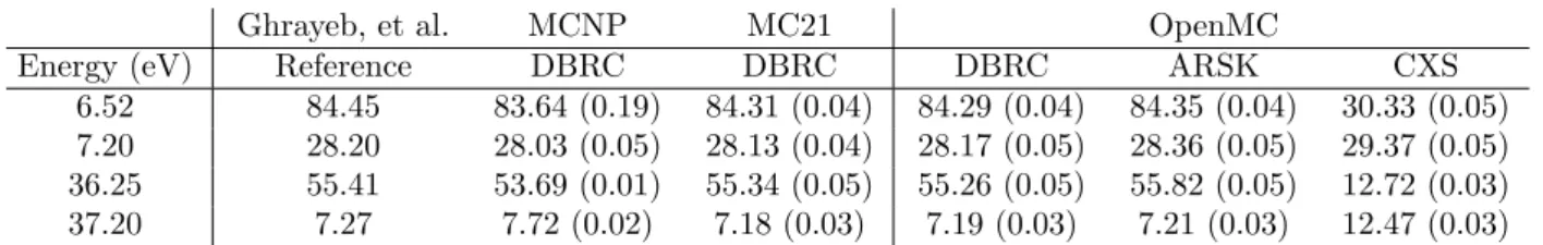
Table 1: Code-to-code comparison of computed upscatter percentages (1σ)
4. RESULTS
The presented results serve two purposes. The first is to verify that the ARSK method does, in fact, correctly reproduce exact scattering kernels, as the DBRC method has been shown to do[4][6][5]. The second is to demonstrate that using the ARSK method in reactor physics simulations results in improved computational performance relative to the DBRC method. In a tangential effort, the newly implemented OpenMC DBRC capability is also verified so that it can be used with confidence in additional verification studies of ARSK for which no reference literature results exist.
As part of the verification of the proposed method, we compare upscatter percentages and mean scattered energies calculated with ARSK to DBRC and deterministic reference results from the literature. Asymp-totic, CXS, DBRC, and ARSK scattering kernels are also computed and compared. In order to assess the computational performance of the new method, we calculate sample target velocity rejection rates at various energies with both the DBRC and ARSK methods. Additionally, pin cell and full core benchmark simula-tions are performed with both methods to quantify efficiency gains that are realized by using ARSK instead of DBRC in calculations of practical interest. The benchmark calculations also serve to further verify ARSK against the DBRC method.
All calculations in this work are performed with ENDF/B-VII.0 nuclear data[23]. In eigenvalue calcula-tions, the specified target velocity sampling method is applied only to238U over the range 5.0-210 eV. The CXS model is applied below this range and the asymptotic model is applied above. The lower energy bound is chosen so that the range includes the lowest-lying238U s-wave resonance at 6.67 eV. Below the selected bound, the error in the scattering kernel that results from invoking the CXS approximation is negligible. The upper bound of the range is chosen to agree with previous benchmark simulations performed with the DBRC method[4]. All other nuclides are treated with the CXS model up to a threshold energy of 400 kT , at which point the asymptotic model is applied.
4.1. Upscatter Percentages
The first verification of ARSK is a comparison of 238U upscatter percentages computed at 1000 K for incident neutron energies just above and just below the 6.67 eV and 36.67 eV resonances. The percentages computed with ARSK are compared with the deterministic results of Ghrayeb, et al.[7] in Table 1. DBRC results computed with MCNP[4], MC21[5], and OpenMC are also presented, along with CXS results from OpenMC. The upscatter percentages computed with ARSK in OpenMC agree very well with both the deterministic and DBRC reference results, especially when compared to the values obtained with the CXS method.
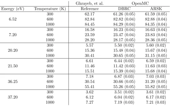
For further verification, upscatter percentages are computed with ARSK at different temperatures for incident neutron energies just above and just below the first three238U s-wave resonances. In Table 2, these
values are compared to deterministic literature results and DBRC results generated with OpenMC. Again, very good agreement is observed between the deterministic, DBRC, and ARSK results.
Though not all of the ARSK upscatter percentages lie within two standard deviations of the reference results, examination of the tabulated values reveals that the various DBRC results often lie several standard deviations away from the reference values, and each other. The differences between the results obtained from the deterministic, DBRC, and ARSK exact scattering kernel implementations are negligible compared to the systematic errors observed in the results computed with the CXS algorithm. In light of the relatively
Ghrayeb, et al. OpenMC
Energy (eV) Temperature (K) Reference DBRC ARSK
300 62.17 61.26 (0.05) 61.59 (0.05) 6.52 600 82.84 82.82 (0.04) 82.88 (0.04) 1000 84.45 84.29 (0.04) 84.35 (0.04) 300 16.58 16.23 (0.04) 16.63 (0.04) 7.20 600 23.59 23.47 (0.04) 23.83 (0.04) 1000 28.20 28.17 (0.05) 28.36 (0.05) 300 5.57 5.50 (0.02) 5.60 (0.02) 20.20 600 15.36 15.48 (0.04) 15.67 (0.04) 1000 30.41 30.65 (0.05) 31.15 (0.05) 300 6.61 6.44 (0.02) 6.59 (0.02) 21.50 600 11.46 11.42 (0.03) 11.63 (0.03) 1000 15.51 15.39 (0.04) 15.68 (0.04) 300 7.18 6.87 (0.03) 7.03 (0.03) 36.25 600 30.54 30.66 (0.05) 31.20 (0.05) 1000 55.41 55.26 (0.05) 55.82 (0.05) 300 3.62 3.51 (0.02) 3.61 (0.02) 37.20 600 6.12 6.04 (0.02) 6.17 (0.02) 1000 7.27 7.19 (0.03) 7.21 (0.03)
Table 2: Comparison of upscatter percentages (1σ) computed with DBRC and ARSK
minor and unbiased differences between the reference, DBRC, and ARSK results, we proceed to the next step in the verification of ARSK.
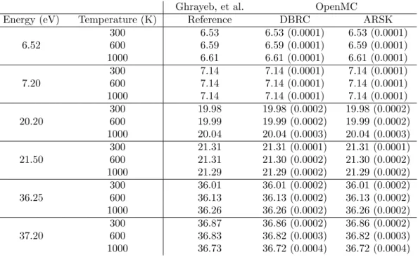
4.2. Mean Scattered Energies
As in the analysis of upscatter percentages, mean scattered energies are computed with ARSK at different temperatures for incident neutron energies just above and just below the first three238U s-wave resonances. Again, the computed values are compared to deterministic literature results and DBRC results generated with OpenMC. In Table 3, very good agreement is seen between scattered energies calculated with ARSK and scattered energies calculated either deterministically or with the DBRC method.
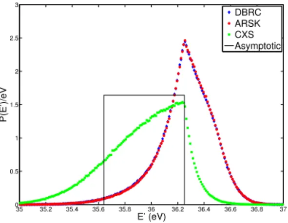
4.3. Scattering Kernels
As a third step in the verification of ARSK, scattering kernels at two energies near the 36.67 eV 238U resonance are computed and plotted, along with the kernels computed with the asymptotic model, and both the CXS and DBRC methods. Figures 1 and 2 illustrate scattering kernels computed for an incident neutron energy of 36.25 eV at 300 K and 1000 K, respectively. The kernels depicted in Figures 3 and 4 are computed for an incident energy of 37.2 eV at 300 K and 1000 K, respectively.
The expected deviation of the CXS, DBRC, and ARSK kernels from the asymptotic kernel is clear in each plot. The discrepancy between the CXS kernel and the exact DBRC and ARSK kernels is also readily apparent. There is very good visual agreement between the DBRC and ARSK kernels in each of the four cases presented. As anticipated, the differences between the exact scattering kernels and the kernels predicted by the asymptotic model are amplified by increases in temperature. Finally, higher probabilities of upscatter are observed for incident energies just below the resonance than are observed for incident energies just above the resonance. All of these general trends are to be expected and have been demonstrated previously[1]. 4.4. Rejection Rates
After a successful verification of ARSK against both the deterministic and DBRC reference results, demonstrated in the preceding comparisons of upscatter percentages, mean scattered energies, and scattering kernel shapes, we transition to an investigation of the computational efficiency of the method. With the
Ghrayeb, et al. OpenMC
Energy (eV) Temperature (K) Reference DBRC ARSK
300 6.53 6.53 (0.0001) 6.53 (0.0001) 6.52 600 6.59 6.59 (0.0001) 6.59 (0.0001) 1000 6.61 6.61 (0.0001) 6.61 (0.0001) 300 7.14 7.14 (0.0001) 7.14 (0.0001) 7.20 600 7.14 7.14 (0.0001) 7.14 (0.0001) 1000 7.14 7.14 (0.0001) 7.14 (0.0001) 300 19.98 19.98 (0.0002) 19.98 (0.0002) 20.20 600 19.99 19.99 (0.0002) 19.99 (0.0002) 1000 20.04 20.04 (0.0003) 20.04 (0.0003) 300 21.31 21.31 (0.0001) 21.31 (0.0001) 21.50 600 21.31 21.30 (0.0002) 21.30 (0.0002) 1000 21.29 21.29 (0.0002) 21.29 (0.0002) 300 36.01 36.01 (0.0002) 36.01 (0.0002) 36.25 600 36.13 36.13 (0.0002) 36.13 (0.0002) 1000 36.26 36.26 (0.0002) 36.26 (0.0002) 300 36.87 36.86 (0.0002) 36.86 (0.0002) 37.20 600 36.83 36.82 (0.0003) 36.82 (0.0003) 1000 36.73 36.72 (0.0004) 36.72 (0.0004)
Table 3: Comparison of mean scattered energies (1σ) (eV) computed with DBRC and ARSK
35 35.2 35.4 35.6 35.8 36 36.2 36.4 36.6 36.8 37 0 0.5 1 1.5 2 2.5 3 E’ (eV) P(E’)/eV DBRC ARSK CXS Asymptotic
35 35.2 35.4 35.6 35.8 36 36.2 36.4 36.6 36.8 37 0 0.5 1 1.5 2 2.5 3 E’ (eV) P(E’)/eV DBRC ARSK CXS Asymptotic
Figure 2: 36.25 eV scattering kernel at 1000 K
35.50 36 36.5 37 37.5 38 0.2 0.4 0.6 0.8 1 1.2 1.4 1.6 1.8 2 E’ (eV) P(E’)/eV DBRC ARSK CXS Asymptotic
Figure 3: 37.2 eV scattering kernel at 300 K
35.50 36 36.5 37 37.5 38 0.2 0.4 0.6 0.8 1 1.2 1.4 1.6 1.8 2 E’ (eV) P(E’)/eV DBRC ARSK CXS Asymptotic
16 17 18 19 20 21 22 23 24 25 26 0 0.1 0.2 0.3 E (eV) Rejections/eV DBRC ARSK 16 17 18 19 20 21 22 23 24 25 26 1e−5 1e−4 1e−3 1e−2 1e−1 1e−0 E (eV) Rejections/eV DBRC ARSK
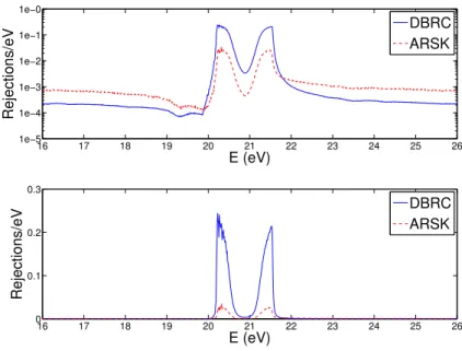
Figure 5: Distribution of rejections in energy (Mosteller pin cell, HFP, 5.0 wt.%)
principle aim of ARSK being to improve upon the rejection sampling scheme employed by the DBRC method, the results presented in this section relate only to the ARSK and DBRC methods.
Because the efficiency of a resonance scattering method depends directly on the number of rejected target velocity samples, the number of rejections per sampled target velocity acceptance is a quantity of particular interest. Moreover, both integral and differential rejection rates can be considered, with the former giving a picture of the overall efficiency of a method and the latter giving information about sampling efficiencies at specific energies. A comparison between the methods’ differential rejection rates is especially enlightening in that it provides some insight as to whether one method performs better in a certain energy range relative to the other method. Analysis of the methods’ relative efficiencies in different energy intervals is necessary if a successful hybrid scheme, which relies on different methods for treating different energies, is to be constructed.
Examination of differential rejection rates also reveals the incident energies that result in the greatest share of total rejections. In any effort to improve overall computational efficiency, attention must be paid primarily to these energies. With this in mind, we look to Figure 5, which shows the distribution over energy of the number of sample target velocity rejections per incident neutron for a pin cell benchmark problem that is described in the next subsection. Resonance scattering is treated in the 5.0-210 eV energy range. For ease of interpretation, Figure 5 displays only the portion of this range that spans the 20.87 eV resonance, as well as energies a few eV above and below.
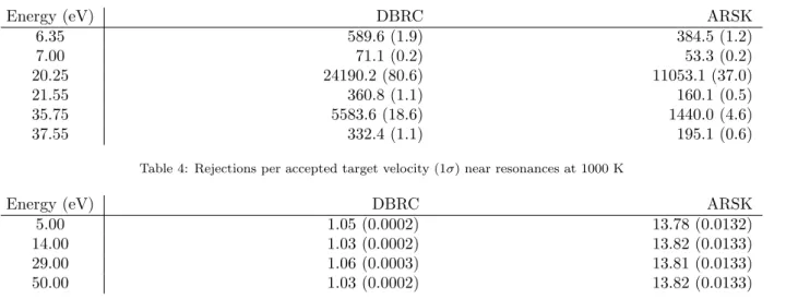
The dependence on energy of the number of observed rejections shown in Figure 5 is representative of behavior seen over the entire energy range in which resonance scattering methods are applied. That is, the majority of rejections occur at energies just above and just below resonances. Away from resonance energies, the number of rejections is relatively minimal. It can also be seen that, in the vicinity of resonances, where most of the rejections occur, the ARSK method requires significantly fewer rejections than does the DBRC method. This is demonstrated in Table 4, which shows the average number of rejections per acceptance at energies near resonances for both the DBRC and ARSK methods. In contrast, away from resonance energies, the DBRC method results in fewer rejections relative to the ARSK method. This is highlighted by the values in Table 5, which shows the average number of rejections per acceptance at energies far from resonances. Taken together, these observations about the relative efficiencies of the two methods lead to the concept of a hybrid method. Such a method can make use of the ARSK method near resonances and
Energy (eV) DBRC ARSK 6.35 589.6 (1.9) 384.5 (1.2) 7.00 71.1 (0.2) 53.3 (0.2) 20.25 24190.2 (80.6) 11053.1 (37.0) 21.55 360.8 (1.1) 160.1 (0.5) 35.75 5583.6 (18.6) 1440.0 (4.6) 37.55 332.4 (1.1) 195.1 (0.6)
Table 4: Rejections per accepted target velocity (1σ) near resonances at 1000 K
Energy (eV) DBRC ARSK
5.00 1.05 (0.0002) 13.78 (0.0132)
14.00 1.03 (0.0002) 13.82 (0.0133)
29.00 1.06 (0.0003) 13.81 (0.0133)
50.00 1.03 (0.0002) 13.82 (0.0133)
Table 5: Rejections per accepted target velocity (1σ) away from resonances at 1000 K
the DBRC method away from resonances. However, because such a vast number of rejections occur near resonances, where ARSK is much more efficient than DBRC, it is likely that this type of hybrid method will lead to no appreciable efficiency gains compared to an ARSK-only approach.
4.5. Pin Cell Benchmark
A set of pin cell benchmark problems was proposed by Mosteller[24] to assess Doppler reactivity defect calculations. The benchmark specifications describe infinite pin cell lattices with low-enriched uranium (LEU) fuel as well as reactor-recycle and weapons-grade mixed-oxide (MOX) fuels. For each type of fuel, multiple compositions are given. Because the benchmark was developed to assess the Doppler reactivity defect, pin cell specifications are given at two different fuel temperatures. At the hot zero-power (HZP) condition, all materials in the problem are at 600 K. At the hot full-power condition (HFP), all materials are again at 600 K, except for the fuel, which is at 900 K. Sunny, et al.[4] used the LEU benchmark problems to investigate the effects of the correct treatment of resonance scattering - via the DBRC method - on Doppler reactivity defect calculations with MCNP. Zoia, et al.[6] and Trumbull and Fieno[5] extended these studies to the MOX fuel types with TRIPOLI and MC21, respectively. Here, the effects of different resonance scattering treatments on the eigenvalues and simulation runtimes of the LEU benchmark problems are investigated.
Differences in keff that result from using the DBRC and ARSK methods to model epithermal scattering
from 238U are shown in Table 6 and compared to the differences calculated with MCNP. In the reference case, relative to which the displayed differences are computed, the CXS model is applied up to an energy of 400 kT . In addition, Table 7 compares the differences in keff calculated with DBRC and ARSK in
OpenMC with those calculated by the TRIPOLI implementation of the DBRC method[6]. In the reference case used for the computation of these differences, the CXS model is applied up to an energy of 210 eV. At both HZP and HFP conditions, agreement between the results produced with the MCNP and OpenMC implementations of DBRC and the results produced with ARSK is very good, as evidenced by nearly all calculated differences lying within one or two standard deviations of each other. Similar agrement is observed for the alternate reference case in which TRIPOLI and OpenMC DRBC results and ARSK results are compared. As anticipated, increased temperature exacerbates the effects of incorrectly modeling epithermal resonance scattering with the CXS model, leading to greater differences between CXS and either DBRC or ARSK eigenvalues.
MCNP OpenMC Enrichment (wt.%) DBRC DBRC ARSK 0.711 -0.00006 (0.00025) -0.00044 (0.00006) -0.00031 (0.00007) 1.6 -0.00071 (0.00035) -0.00056 (0.00010) -0.00077 (0.00010) 2.4 -0.00038 (0.00038) -0.00068 (0.00012) -0.00062 (0.00012) HZP 3.1 -0.00073 (0.00040) -0.00073 (0.00013) -0.00083 (0.00013) 3.9 -0.00087 (0.00040) -0.00094 (0.00014) -0.00079 (0.00014) 4.5 -0.00048 (0.00041) -0.00078 (0.00015) -0.00086 (0.00015) 5.0 -0.00115 (0.00042) -0.00072 (0.00015) -0.00092 (0.00015) 0.711 -0.00057 (0.00027) -0.00111 (0.00008) -0.00109 (0.00008) 1.6 -0.00182 (0.00035) -0.00151 (0.00009) -0.00147 (0.00009) 2.4 -0.00164 (0.00037) -0.00186 (0.00012) -0.00166 (0.00011) HFP 3.1 -0.00155 (0.00038) -0.00161 (0.00012) -0.00171 (0.00012) 3.9 -0.00140 (0.00041) -0.00184 (0.00013) -0.00187 (0.00014) 4.5 -0.00194 (0.00040) -0.00183 (0.00015) -0.00177 (0.00014) 5.0 -0.00154 (0.00040) -0.00185 (0.00015) -0.00156 (0.00015)
Table 6: LEU pin cell keffdifferences (1σ) relative to the CXS case applied below 400 kT
TRIPOLI OpenMC Enrichment (wt.%) DBRC DBRC ARSK 0.711 -0.00066 (0.00013) -0.00070 (0.00006) -0.00057 (0.00007) 1.6 -0.00113 (0.00014) -0.00081 (0.00011) -0.00102 (0.00011) 2.4 -0.00110 (0.00014) -0.00115 (0.00012) -0.00109 (0.00012) HZP 3.1 -0.00115 (0.00016) -0.00103 (0.00014) -0.00113 (0.00014) 3.9 -0.00102 (0.00016) -0.00140 (0.00013) -0.00125 (0.00013) 4.5 -0.00099 (0.00017) -0.00122 (0.00014) -0.00130 (0.00013) 5.0 -0.00115 (0.00017) -0.00111 (0.00014) -0.00131 (0.00014) 0.711 -0.00123 (0.00013) -0.00140 (0.00007) -0.00138 (0.00007) 1.6 -0.00163 (0.00014) -0.00189 (0.00009) -0.00185 (0.00010) 2.4 -0.00225 (0.00014) -0.00207 (0.00012) -0.00187 (0.00012) HFP 3.1 -0.00203 (0.00016) -0.00213 (0.00013) -0.00223 (0.00013) 3.9 -0.00219 (0.00016) -0.00231 (0.00013) -0.00234 (0.00014) 4.5 -0.00222 (0.00016) -0.00230 (0.00014) -0.00224 (0.00013) 5.0 -0.00224 (0.00017) -0.00266 (0.00014) -0.00237 (0.00014)
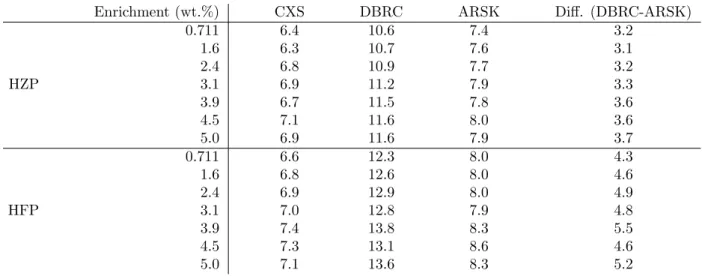
Enrichment (wt.%) CXS DBRC ARSK Diff. (DBRC-ARSK) 0.711 6.4 10.6 7.4 3.2 1.6 6.3 10.7 7.6 3.1 2.4 6.8 10.9 7.7 3.2 HZP 3.1 6.9 11.2 7.9 3.3 3.9 6.7 11.5 7.8 3.6 4.5 7.1 11.6 8.0 3.6 5.0 6.9 11.6 7.9 3.7 0.711 6.6 12.3 8.0 4.3 1.6 6.8 12.6 8.0 4.6 2.4 6.9 12.9 8.0 4.9 HFP 3.1 7.0 12.8 7.9 4.8 3.9 7.4 13.8 8.3 5.5 4.5 7.3 13.1 8.6 4.6 5.0 7.1 13.6 8.3 5.2
Table 8: LEU pin cell runtime overhead (%)
overhead percentages2that are observed when the OpenMC implementations of the CXS, DBRC, and ARSK methods are applied over the 5.0-210 eV energy range. For each combination of enrichment, temperature, and resonance scattering method, the percentage value is calculated using the median runtime out of eight independent serial simulations. Comparable results are obtained when the average runtime is used instead of the median value. With the ARSK method, we see runtime overhead of 7-8%. Depending on enrichment and temperature, this amounts to a 30-40% reduction in the runtime overhead compared to the DBRC method. The efficiency gains realized by applying ARSK instead of DBRC in the epithermal region are greater at HFP conditions than at HZP conditions. Also, for a given temperature, the efficiency of ARSK, relative to DBRC, improves slightly with increasing enrichment. Only a small increase in runtime - approximately 1% - is observed when switching from the CXS method to ARSK.
Extending the energy range over which the CXS method is applied from 400 kT up to 210 eV results in runtime overheads of 6-7%. This, taken along with the observation that the inaccuracies in computed eigenvalues that occur as a result of the application of the CXS approximation actually increase as the energy range is extended, supports a determination that there is no clear, practical advantage to using the CXS method in an attempt to account for resonance scattering effects induced by the thermal motion of target nuclei. Indeed, there are clear, practical disadvantages of increased runtime and greater inaccuracy in calculated eigenvalues. Because the CXS method explicitly neglects the root cause of resonance scattering effects (i.e. the dependence of cross sections on energy), the ineffectiveness of applying the approximation to resonant scatterers over a broader energy range is not unexpected.
4.6. Full Core Benchmark
In the interest of assessing the performance of the ARSK method in full core reactor simulations, eigen-value calculations are carried out with the three-dimensional BEAVRS model[25]. Differences in keff and
runtime overhead at both HZP and HFP conditions are displayed in Tables 9 and 10, respectively. As in the analysis of pin cell runtimes, overhead percentage values2 are calculated using the median runtime out of eight independent serial simulations.
The keff values calculated with DBRC and ARSK are in very good agreement. The gains in runtime
efficiency realized when using ARSK, rather than DBRC, in the full core problem are somewhat lower than in the pin cell calculations presented earlier. This is likely due to the dependence of runtime on the
2Percentages are calculated relative to a standard reference case in which the CXS approximation is applied below 400 kT .
At HZP and HFP conditions, 400 kT corresponds to 20.68 eV and 31.02 eV, respectively. The asymptotic model is applied above the 400 kT cutoff.
CXS DBRC ARSK
HZP 0.00025 (0.00005) -0.00050 (0.00005) -0.00048 (0.00006)
HFP 0.00029 (0.00005) -0.00137 (0.00005) -0.00140 (0.00005)
Table 9: BEAVRS keff differences (1σ) relative to the CXS case applied below 400 kT
CXS DBRC ARSK Diff. (DBRC-ARSK)
HZP 4.0 4.6 4.0 0.6
HFP 4.9 8.7 6.0 2.7
Table 10: BEAVRS runtime overhead (%)
performance of the code as a whole and not simply on the resonance scattering treatment. The full core benchmark requires tracking of particles across many more cells and materials than are present in the pin cell benchmarks. This increases the relative fraction of runtime spent performing operations unrelated to resonance scattering and, in doing so, reduces the runtime overhead attributable to resonance scattering treatments. Even so, at HFP conditions for the three-dimensional, full core BEAVRS model, a 2.7% reduc-tion in absolute runtime is achieved by utilizing the proposed ARSK method instead of the DBRC. This is a 31% reduction in runtime overhead. Both the pin cell and full core investigations of the ARSK method focus only on resonance scattering in238U. When several additional resonant nuclides are included in the
resonance scattering treatment, as in depletion calculations, the efficiency gains of ARSK may be somewhat amplified.
5. CONCLUSIONS
A new method for the exact treatment of epithermal resonance scattering in Monte Carlo neutron transport codes is presented. The proposed ARSK method is verified against reference upscatter probability and mean scattered energy results in the literature. Differences in eigenvalues that result from applying the exact DBRC and ARSK resonance scattering methods, instead of the CXS approximation, are shown to be in excellent agreement with reference literature results for the Mosteller LEU pin cell benchmark problems. Differences in the eigenvalues for the three-dimensional, full core BEAVRS model computed with the OpenMC implementations of DBRC and ARSK are also in excellent agreement with each other. Comparisons between DBRC and ARSK rejection rates show that ARSK requires many fewer rejections near resonances than does DBRC. Further, the large reduction in the number of rejections near resonances that is observed with the ARSK method is shown to reduce overall runtimes by 3-5% relative to the DBRC method for problems of practical interest. In both pin cell and full core benchmark simulations, this corresponds to a 30-40% reduction in runtime overhead.
6. ACKNOWLEDGMENTS
The authors thank Paul K. Romano for spurring the addition of helpful clarifications to this article with his comments and suggestions.
This research was partially supported by the Consortium for Advanced Simulation of Light Water Reac-tors (www.casl.gov), an Energy Innovation Hub (http://www.energy.gov/hubs) for Modeling and Simulation of Nuclear Reactors under U.S. Department of Energy Contract No. DE-AC05-00OR22725.
This material is based upon work partially supported under appointment of the first author to a Depart-ment of Energy Nuclear Energy University Programs Graduate Fellowship.
References
[1] M. Ouisloumen, R. Sanchez, A model for neutron scattering off heavy isotopes that accounts for thermal agitation effects, Nuclear Science and Engineering 107.3 (1991) 189–200.
[2] L. L. Carter, E. D. Cashwell, Particle-Transport Simulation with the Monte Carlo Method, TID-26607, ERDA Critical Review Series, U. S. Energy Research and Development Administration, Technical Information Center, Oak Ridge, TN, 1975.
[3] P. K. Romano, B. Forget, The OpenMC Monte Carlo particle transport code, Annals of Nuclear Energy 51 (2013) 274–281.
[4] E. E. Sunny, F. B. Brown, B. C. Kiedrowski, W. R. Martin, Temperature effects of resonance scattering for epithermal neutrons in MCNP, in: Proc. Int. Conf. on the Physics of Reactors: Advances in Reactor Physics (PHYSOR 2012), 2012. [5] T. H. Trumbull, T. E. Fieno, Effects of applying the Doppler broadened rejection correction method for LEU and MOX
pin cell depletion calculations, Annals of Nuclear Energy 62 (2013) 184–194.
[6] A. Zoia, E. Brun, C. Jouanne, F. Malvagi, Doppler broadening of neutron elastic scattering kernel in TRIPOLI-4, Annals of Nuclear Energy 54 (2013) 218–226.
[7] S. Z. Ghrayeb, M. Ouisloumen, A. M. Ougouag, K. N. Ivanov, Deterministic modeling of higher angular moments of resonant neutron scattering, Annals of Nuclear Energy 38 (2011) 2291–2297.
[8] J. J. Duderstadt, L. J. Hamilton, Nuclear Reactor Analysis, Wiley, 1976.
[9] D. Lee, K. Smith, J. Rhodes, The impact of238U resonance elastic scattering approximations on thermal reactor Doppler
reactivity, Annals of Nuclear Energy 36.3 (2009) 274–280.
[10] D. E. Cullen, C. R. Weisbin, Exact Doppler broadening of tabulated cross sections, Nuclear Science and Engineering 60.3 (1976) 199–229.
[11] W. Rothenstein, Neutron scattering kernels in pronounced resonances for stochastic Doppler effect calculations, Annals of Nuclear Energy 23 (1996) 441–458.
[12] E. M. Gelbard, Epithermal Scattering in VIM, FRA-TM-123, Argonne National Laboratory, 1979.
[13] X-5 Monte Carlo Team, MCNP A General Monte Carlo N-Particle Transport Code, Version 5, LA-UR-03-1987, Los Alamos National Laboratory, 2008.
[14] T. M. Sutton, T. J. Donovan, T. H. Trumbull, P. S. Dobreff, E. Caro, D. P. Griesheimer, L. J. Tyburski, D. C. Carpenter, H. Joo, The MC21 Monte Carlo code, in: Proc. Int. Conf. on Mathematics & Computations and Supercomputing in Nuc. Applications, 2007.
[15] R. E. Macfarlane, D. W. Muir, The NJOY Nuclear Data Processing System, Version 91, LA-12740-M, Los Alamos National Laboratory, 1994.
[16] W. Rothenstein, Proof of the formula for the ideal gas scattering kernel for nuclides with strongly energy dependent scattering cross sections, Annals of Nuclear Energy 31 (2004) 9–23.
[17] R. Dagan, On the use of S(α, β) tables for nuclides with well pronounced resonances, Annals of Nuclear Energy 32 (2005) 367–377.
[18] B. Becker, On the Influence of the Resonance Scattering Treatment in Monte Carlo Codes on High Temperature Reactor Characteristics, Ph.D. thesis, University of Stuttgart, Germany, 2010.
[19] D. E. Cullen, Program SIGMA1 (Version 79-1): Doppler Broaden Evaluated Cross Sections in The Evaluated Nuclear Data File/Version B (ENDF/B) Format, UCRL-50400, Vol. 17, Part B, Rev. 2, Lawrence Livermore Laboratory, 1979. [20] B. Becker, R. Dagan, G. Lohnert, Proof and implementation of the stochastic formula for ideal gas, energy dependent
scattering kernel, Annals of Nuclear Energy 36 (2009) 470–474.
[21] Tripoli-4 Project Team, 2008, Tripoli-4 User Guide, CEA-R-6169, French Alternative Energies and Atomic Energy Com-mission, 2008.
[22] T. Mori, Y. Nagaya, Comparison of resonance elastic scattering models newly implemented in MVP continuous-energy Monte Carlo code, Journal of Nuclear Science and Technology 46.8 (2009) 793–798.
[23] M. B. Chadwick, P. Oblozinsky, M. Herman, et al., ENDF/B-VII.0: next generation evaluated nuclear data library for nuclear science and technology, Nuclear Data Sheets 107 (2006) 2931–3060.
[24] R. D. Mosteller, Computational Benchmarks for the Doppler Reactivity Defect, LA-UR-06-2968, Los Alamos National Laboratory, 2006.
[25] N. Horelik, B. Herman, B. Forget, K. Smith, Benchmark for evaluation and validation of reactor simulations (BEAVRS), in: Proc. Int. Conf. on Mathematics and Computational Methods Applied to Nuclear Science and Engineering (M&C 2013), 2013.