Publisher’s version / Version de l'éditeur: Student Report, 2010-12-20
READ THESE TERMS AND CONDITIONS CAREFULLY BEFORE USING THIS WEBSITE.
https://nrc-publications.canada.ca/eng/copyright
Vous avez des questions? Nous pouvons vous aider. Pour communiquer directement avec un auteur, consultez la première page de la revue dans laquelle son article a été publié afin de trouver ses coordonnées. Si vous n’arrivez pas à les repérer, communiquez avec nous à [email protected].
Questions? Contact the NRC Publications Archive team at
[email protected]. If you wish to email the authors directly, please see the first page of the publication for their contact information.
NRC Publications Archive
Archives des publications du CNRC
For the publisher’s version, please access the DOI link below./ Pour consulter la version de l’éditeur, utilisez le lien DOI ci-dessous.
https://doi.org/10.4224/17210709
Access and use of this website and the material on it are subject to the Terms and Conditions set forth at
Development of an ice sheet scheduling package
Smith, Jordan
https://publications-cnrc.canada.ca/fra/droits
L’accès à ce site Web et l’utilisation de son contenu sont assujettis aux conditions présentées dans le site LISEZ CES CONDITIONS ATTENTIVEMENT AVANT D’UTILISER CE SITE WEB.
NRC Publications Record / Notice d'Archives des publications de CNRC:
https://nrc-publications.canada.ca/eng/view/object/?id=22b19e8b-8e02-47e0-89c7-9220f2fb32d9 https://publications-cnrc.canada.ca/fra/voir/objet/?id=22b19e8b-8e02-47e0-89c7-9220f2fb32d9
DOCUMENTATION PAGE
REPORT NUMBER SR-2010-26
NRC REPORT NUMBER DATE
December 2010 REPORT SECURITY CLASSIFICATION
Unclassified
DISTRIBUTION Unlimited TITLE
DEVELOPMENT OF AN ICE SHEET SCHEDULING PACKAGE AUTHOR(S)
Jordan Smith
CORPORATE AUTHOR(S)/PERFORMING AGENCY(S)
Institute for Ocean Technology, National Research Council, St. John’s, NL PUBLICATION
SPONSORING AGENCY(S)
IOT PROJECT NUMBER NRC FILE NUMBER
KEY WORDS
Ice Tank, Ice Sheet Scheduler, Software, SEG, SQL server 2005, Python, matplotlib, wxPython, pyODBC, pymssql PAGES ii, 19, App. A FIGS. 4 TABLES SUMMARY
The facilites at the National Research Council of Canada’s Institute for Ocean Tech- nology allow for testing of marine models in ice. Ice properties collected during the creation and testing of each ice sheet are currently stored digitally using outdated architecture. New software and databases are being developed to replace present
systems. Of the components being updated, a program which facilitates the scheduling of ice sheets is of particular focus.
National Research Council Conseil national de recherches Canada Canada Institute for Ocean Institut des technologies
Technology océaniques
DEVELOPMENT OF AN ICE SHEET
SCHEDULING PACKAGE
SR-2010-26 Jordan Smith December 2010
SR-2010-26
EXECUTIVE SUMMARY
Facilities at the National Research Council of Canada’s Institute for Ocean
Technology allow for testing of marine models in ice. Ice properties
col-lected during creation and testing of each ice sheet are currently stored
digitally using outdated architecture. New software and databases are
be-ing developed to replace present systems. In particular, a program which
facilitates the scheduling of ice sheets has been recently developed.
Current ice sheet scheduling tools include empirical equations, data
stor-age systems, and their software. During the months of September to
December 2010 older VMS scheduling routines written for DEC
DATA-TRIEVE were examined and a replacement was written using the modules
matplotlib, wxPython and pyODBC for the Python programming language
along with a Microsoft SQL Server 2005 database.
Development followed a traditional design process of gathering
specifica-tions, prototyping, and testing. Developers of the older system were
con-sulted, along with its current users. Documentation and source code were
also reviewed. Specifications were drafted using the collected information,
SR-2010-26 CONTENTS
Contents
1 Tools 3
1.1 Equations . . . 4
1.2 Data and Software Tools . . . 4
2 Design Objectives and Requirements 6 2.1 Original Software System . . . 6
2.2 User Comments on Original VMS System . . . 6
2.3 Technical Specifications . . . 7
3 Development 8 3.1 Gathering Requirements . . . 8
3.2 Package Choice . . . 8
3.3 Design and Prototyping . . . 9
3.4 Implementation . . . 10
4 Suggestions 14 4.1 On Producing Better Models . . . 14
4.2 Expanding the system . . . 15
4.3 Optimizations in Prediction . . . 16
4.4 Optimized Scheduling . . . 16
4.5 Expanding the new Data set . . . 17
References 19
Appendices 20
A Sample code: matplotlib + wxPython A-1
SR-2010-26 CONTENTS
Introduction
Established by the National Research Council (NRC) in 1985, the large
refrigerated model testing tank (the ’Ice Tank’) at the Institute of Ocean
Technology (IOT) has the capability of producing ice covers between 5
and 160 mm (and occasionally thicker). It requires, among other things,
chilling 3.24 million litres of water, then freezing the expansive room in
which the tank is housed to temperatures as cold as -30◦C, followed by
blast reheating the room to condition the ice to appropriate strengths for
testing. These are expensive activities which require significant energy
consumption, specialized staff and finely calibrated equipment; errors in
the freezing process also carry the risk of damaging the tank, testing
car-riages or building structure. As such, it is very important that accurate
estimates of timings, required resources, staff and conditions are available
to tank operators.
Scheduling of ice tank operations is done using a variety of tools
in-cluding, but not limited to, manual analysis of historical data, archival,
an-alytical, and retrieval software systems, empirical equations and
spread-sheet macros. Some of these tools have weaknesses, such as
inaccu-racy, reliance on outdated architecture or programming languages,
SR-2010-26 1 TOOLS
1
Tools
To date (December 2010), over 1100 ice sheets have been grown at IOT.
These have included several types of ice coverings. Different mechanical
manipulations of the final ice product for model testing can simulate
differ-ent natural ice formations including the default level ice testing, pre-sawn
ice, pack ice, ice rubble fields, ’dump-truck’ ridges, thin layered ridges, thick
layered ridges and rafted over rubble. Chemical composition of the
solu-tion from which ice is grown can also be varied, as well as density of the
ice by bubbling air throughout the tank during freezing. This leads to 4
de-fault types of ice: doped model ice (known as ’EGADS ice’, as it contains
Ethylene Glycol, Aliphatic Detergent and Sugar), bubbled model ice (aka
corrected density / CD ice), fresh ice (extremely tough ice) and unseeded
(ice with irregular/natural crystal growth ice is otherwise ’seeded’ with a
water mist at start of freeze to promote uniform vertical crystal growth).
Also, a variety of mechanical testing is done on the sheet to determine
physical properties of the ice; this information is manually recorded onto
paper charts, then transferred to the computer later, though there are
SR-2010-26 1 TOOLS
1.1
Equations
Coupled with research done in late 80’s, in-house experiments and
analy-ses were completed to develop new models for predicting thin ice growth.
These involved analysis of 384 doped ice sheets and 30 freshwater sheets
completed by 1986. (Lozowski, Jones, Hill 1990). This research, coupled
with regression analysis of tempering curves and growth rates yielded a
set of 3 equations for ice growth, and another 3 for ice tempering. (See
appendix) These equations are commonly used for initial estimates and
rough costing or planning. They are indispensable tools for creating
time-lines and provide reasonable accuracy but unfortunately do not take into
account recent developments in ice sheet processes and current
condi-tions. Factors such as minor changes in dopant concentrations, the effect
of bubbling in the commonly used CD ice and other predictable
discrep-ancies change required freezing conditions and require adjustments. For
this reason, equations are not the only tool available and a combination
of tools are usually required to produce final schedules, costing estimates
and determine what staff must be on hand during specified time periods.
1.2
Data and Software Tools
Scheduling software and data systems represent another critical resource.
As tests are completed on an ice sheet a multitude of information about the
sheet is recorded, then analyzed and stored by a software system. The
system which is currently in use is based on VAX/VMS architecture and the
SR-2010-26 1 TOOLS
DEC DATATRIEVE database. Terminal-based FORTRAN and DATARIEVE
procedures are used by several packages in the Ice Analysis, Scheduling,
Bubbler and data collection systems. At time of writing, work is
under-way to move from the VMS system to new architecture. A great deal of
data has been ported to MS SQL Server 2005 databases and new
soft-ware suites to analyze and enter data have been written to interface with
them. The original systems created by Brian Hill, Donald Spencer and
David Molyneux were extensively studied, source code reviewed and
doc-umentation consulted. In addition, meetings with Ice tank staff were held to
determine current use of software and requirements of the new systems.
A new software suite was designed by the IOT software engineering group
with Greg Janes, Wayne Pearson and Michael Sullivan’s leads in primarily
C#, SQL (Structured Query Language) and Python to meet storage and
analysis needs of tank operators. In addition, reporting and scheduling
systems were created using the Python programming language, pyODBC
and pymssql database interface packages, wxPython Graphical User
In-terface (GUI) toolkit, ReportLab PDF library and plotting/math package
matplotlib. These software systems allow for easy entry and retrieval of
historical ice tank data, analysis of results and graphical feedback. The
scheduling tools in particular allow for far more precise results in
SR-2010-26 2 DESIGN OBJECTIVES AND REQUIREMENTS
2
Design Objectives and Requirements
2.1
Original Software System
The primary purpose of the original scheduling software was to facilitate
easy and fast access to historical data. It was structured in such a way as
to be precise without frequent regression analysis of data or reformulation
of equations and to allow operator’s discretion in what data was
consid-ered such as ignoring outliers. The simplest way to do with was to retrieve
data which had been filtered by a user’s required parameters, then plotting
it in the same way tempering curves are plotted. A user could then
pre-form graphical approximation without time-consuming procedural removal
of outliers during a computer’s curve fit or analyze clusters of data to
ob-serve trending. This would allow a user to include newer sheet data for
more accurate estimations, something which the empirical equations do
not allow.
2.2
User Comments on Original VMS System
Users of the current system note that the iterative procedural nature of the
program makes using DATATRIEVE routines time-consuming. Using the
scheduler requires that a user run up to 4 programs consecutively from
the terminal, iterating any time they make a mistake, wish to retrieve more
data or refine their search. Plots which are created are monochrome,
provide little user interaction or analysis of points, require knowledge of
SR-2010-26 2 DESIGN OBJECTIVES AND REQUIREMENTS
DATATRIEVE plotting commands and data returned can be ambiguous or
imprecise.
2.3
Technical Specifications
The new system is centred around a 2005 Microsoft SQL Server Database
and requires any software developed around it be compatible. The new
scheduler software achieves this using the pyODBC package for the Python
scripting language which allows execution of SQL queries and procedures
using Open DataBase Connectivity and Python Database API
Specifica-tion v2.0 interfaces. A Graphical User Interface (GUI) was created using
the wxPython toolkit and plotting/math package matplotlib was used for
SR-2010-26 3 DEVELOPMENT
3
Development
3.1
Gathering Requirements
As per traditional design methodology the first step in developing a new
scheduler was to create a specification that it must satisfy. These were
obtained by analyzing technical constraints such as type and version of
database that must be accessed, the programming language(s) which
were to be used, and chosen deployment MS SQL Server 2005, Python
and Windows XP GUI, respectively. Clients suggested interactive
plot-ting capability, a high degree of user control or filtering and simple, fast
use were important characteristics. In addition, libraries must be free to
work with, highly capable, have a sufficient level of support or
documen-tation and be familiar to other developers. Consuldocumen-tation with developers of
the previous software, available documentation and source code defined
certain functionality which should not be removed, along with details of
software particulars.
3.2
Package Choice
To meet these needs several open source python packages were
cho-sen. In selecting a module for database connectivity there were several
choices, the most promising of which were pyODBC and pymssql. Upon
viewing documentation, online discussions, source code and testing both
packages, pyODBC was chosen. The ODBC module promised continued
SR-2010-26 3 DEVELOPMENT
development, compliance with more standards, more versions, read from
the database easily and supposedly had more features, despite lacking in
several important areas continued support, compliance and possible
fu-ture bug-fixes made it a better choice to support fufu-ture development. The
other module, pymssql on the other hand was implemented much better,
the features it did include were far superior to pyODBC and it worked
with-out problem. Unfortunately it appeared to be reaching the end of it’s
life-time and there were suggestions that it would no longer work if any other
component of the system were to be upgraded, including the database
and other programming libraries. Matplotlib and wxPython were chosen
because of familiarity with the products, ample support, ease of use and
a wide variety of features. Competitor GUI toolkits such as TK were said
to be harder to work with and all alternatives to matplotlib were much less
mature in their development.
3.3
Design and Prototyping
Once a platform for production was chosen the user interface was drafted.
Several rough sketches were created to test layout, look and feel, as well
as functionality. Once particulars were determined a graphical interface
was prototyped. To support the interface a backend for processing user
var-SR-2010-26 3 DEVELOPMENT
end appeared in the GUI, and interface events such as button presses
and user selections triggered appropriate responses and updates from the
backend.
3.4
Implementation
Development of the scheduler was centred around ease of use. The
pre-vious software was very time-consuming and tricky for current users who
are unfamiliar to DATATRIEVE commands or used to a Graphical User
In-terface. As such, attempts were made to make it possible to navigate using
a mouse exclusively, but also allow users to navigate with the keyboard.
Because of this there are many SpinControls in the interface.
(SpinCon-trols are text boxes which allow keyboard entry of numbers, but also allow
increasing or decreasing the value by clicking on up and down arrows next
to the the form). Certain portions of the previous system were merged in
this design, making the interface less cluttered and faster to use. Where it
once required entering answers to a series of questions before displaying
output, a user can now click on a few controls and see results instantly.
When the program is run, the first thing it does before loading any large
modules, is produce a ’splash screen’ image (Fig. 1) from a few lines of
stored code and display it to the user to let them know the program is
in-deed running and has not ’frozen’.
SR-2010-26 3 DEVELOPMENT
Figure 1: Result of importing splash.py
Figure 2: Blank fields of GUI on initalization
This is done to prevent multiple attempts at initialization in the event of
a slow loading process. On top of this image the main GUI is loaded as
a separate application. (Fig.2) On startup the GUI contains many blank
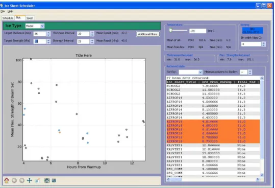
SR-2010-26 3 DEVELOPMENT
Figure 3: Demonstrations of various graphical feedback
As data is entered it triggers color changes, as when choosing ice type
the background of the control turns white for bubbled, blue for fresh, etc.
When choosing temperature, cold temperatures turn a display blue while
warm turn it orange. This reminds a user of what action they have taken,
or whether they have set a particular parameter. Also, as each filtering
pa-rameter is set, new filters are applied to the query sent to the database and
a reload of the plot is triggered as well as the tabular display of returned
data. Other changes occur when a user interacts with the plot area. The
toolbar at the bottom of the plot allows a user to ’zoom in’ on portions of
clustered data, move the section around or return the plot to it’s initial
SR-2010-26 3 DEVELOPMENT
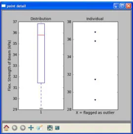
Figure 4: Distribution of values within a test at a single location
dition. If a user moves their cursor over a data point the group of related
points (those tests within the same ice sheet) are highlighted, as well as
text which gives particular details of that sheet. This aids in identifying
individual tempering curves, mentally sorting large clusters of data and
matching details to ambiguous points so users may apply more
appropri-ate filters. In addition, if a user right-clicks on a point, a menu is displayed
(Fig. 4) showing membership details of that point and giving the option of
breaking the point into it’s constituent parts. The ’point details’ option of
the menu launches a box plot and scatter plot of the beam strengths which
have been averaged to create a single point on the main plot. This is very
useful in identifying outliers and finding the source of problems within a
SR-2010-26 4 SUGGESTIONS
4
Suggestions
Tank operators have become very familiar with the original software
sys-tems and data handled by them. As such they have offered several
sug-gestions on how the scheduling process could be improved, along with the
software which facilitates it. Current development is an opportune time to
act on these suggestions and implement them in a functional system. In
addition to these suggestions, various other things were noted during the
development process by developers which may help in future
advance-ment of the software.
4.1
On Producing Better Models
It may be possible to flag outlying data as new data is entered into the
sys-tem and have a computer perform regression analysis to produce better
equations, automatically presenting more accurate results while
remov-ing errors caused by manual approximations. Alternatively, as many more
sheets have been completed since the inception of the original systems
and models of ice growth, more precise modern models could be created.
Also, due to the nature of the sheets being completed at the time, the
orig-inal system did not discriminate between different ice types and different
uses; variations in chemical and physical composition were not taken into
account and it is known to greatly affect current models and equations.
SR-2010-26 4 SUGGESTIONS
4.2
Expanding the System
Other data may be available in physical records, that is not kept in our
database. This includes the results of concentration testing done
period-ically to determine dopant and contamination levels or when refilling the
tank with new solution. There is evidence that the effect on initial
freez-ing is minimal, but these dopants do affect other parts of the ice sheet
creation cycle and model testing. In addition to EGADS there are
particu-lar density test results which are invaluable in calibration which are rarely
recorded and have not been kept as part of ice tank archives. Users also
suggested allowing a comment field for each sheet summary to review the
overall quality of the sheet and mark anomalies or fixes. Also related to
ex-pansion is a comment that particular test results, such as friction, are not
necessarily tied to a particular sheet, for example testing of experimental
new hull coatings which are not applied to models - it would be of benefit
if a parallel, rather than integrated system were to handle this. Also, given
the relative cheap cost of modern storage, it would be of benefit to begin
storing images taken in association with an ice sheet, such as those
an-alyzed to determine ice covering concentrations in pack ice testing which
are usually given to students for analysis, then lost.
SR-2010-26 4 SUGGESTIONS
Sections of the freeze cycle which occur during the large temperature
changes of initial cooling and warmup have traditionally been accounted
for with straight line approximation when in fact they demonstrate
New-tonian cooling/heating curves or could be calculated though integrals of
curves from temperature records. It is possible that this was originally
done as blast heating modifies the curve to a more linear result, though
times of heating are recorded and division of the curves is possible if
re-quired. This modification would not only increase accuracy of prediction,
but allow for cost savings: curves could be extrapolated to test time to
minimize the amount of costly blast heat required to temper ice quickly.
4.4
Optimized Scheduling
It has also been suggested that a scheduling tool might include capabilities
for planning multiple sheets in the same session. It may be possible to, for
example, outline the specifics of project’s individual sheets, then use this
information to plan all relevant tests within the project, bearing in mind
per-sonnel schedules, overtime requirements and other preferences. It would
also be possible to print monthly schedules (perhaps as pdf output with
ReportLab and other packages) or calendar entries for Outlook, Google
Calendar or Rainlendar.
SR-2010-26 4 SUGGESTIONS
4.5
Expanding the New Data Set
It would be very beneficial to add more of the available data to the database
as parsers for such material have already been written and storage is
read-ily available. Currently, certain features are restricted to approximately 200
of the most recent sheets (of the some 1100 completed). Any analysis
for generating new equations or improving scheduling or current
predic-tive capabilities are lacking with the current data set. The modern
collec-tion, though containing newer data and more raw data than before,
cov-ers fewer sheets than 1988’s data set. In particular, the database table
tblIceSheet should be completed, and filling of key matched data spaces
found in tblBeam, tblThickness and tblDensity would be invaluable. Doing
this would require little more effort than requesting archived text files from
Computer systems and running parsers on archived files. Small changes
to parsers could be made in similar way to original development viewing
FORTRAN source to determine format and appending parser
dictionar-ies. This data would allow users to view data in finer resolution when
scheduling and doing other activities (currently this capability is limited to
the aforementioned range). The extra data would also be valuable in model
development. Another important set of data would be the run information
SR-2010-26 4 SUGGESTIONS
reports such as tank diagrams. It would provide a reference for ice
proper-ties which are currently dissociated from testing. This would allow a client
to see the condition of the ice in the location and time window of the test,
which is an important connection when analyzing model test results.
4.6
Conclusions
This development proved to be a significant undertaking requiring more
time than initially thought. Also, as the scheduler is being updated
any-way, it would have been beneficial to concurrently update the models and
algorithms used to predict required freezing and tempering times. As the
current scheduler stands, though the result is useable, there is significant
room for refinement. Further work should be done on the system before
it is deployed as accuracy and reliability is important. As well, results
re-turned from the new system have not been verified to agree with the older
system and caution should be taken when interpreting them. Choices
made with regards to packages and platforms appear to be reasonable,
with the exception of pyODBC (the database connectivity module) and
new developments in this packages should be monitored. As with using
any new module, one must weigh the current condition of the code base,
documentation and future support before one chooses to develop using
that tool.
SR-2010-26 REFERENCES
References
[1] B. T. Hill, “Procedures for scheduling ice sheets,” Tech. Rep.
LM-2007-03, National Research Council Institute For Ocean Technology, April
2007.
[2] B. T. Hill, “Vms ice analysis procedures and preparation of ice sheet
summaries,” Tech. Rep. LM-2006-05, National Research Council
Insti-tute For Ocean Technology, March 2006.
[3] E. P. Lozowski, S.J.Jones, and B. T. Hill, “Labratory measurements of
growth in thin ice and flooded ice,” Cold Regions Science and
Technol-ogy, vol. 20, pp. 25–37, May 2006.
[4] B. T. Hill, “Environmental modeling - ice,” Tech. Rep.
42-8595-S/GM-4, National Research Council Institute For Ocean Technology, January
2008.
[5] J. Smart, R. Roebling, V. Zeitlin, R. Dunn, and et al, wxWidgets 2.8.11:
A portable C++ and Python GUI toolkit. wxWidgets team, 2.8.11 ed.,
February 2010.
[6] D. Dale, M. Droettboom, E. Firing, and J. Hunter, Matplotlib
SR-2010-26
Appendices
SR-2010-26 A SAMPLE CODE: MATPLOTLIB + WXPYTHON
A
Sample code: matplotlib + wxPython
1 from __future__ import print_function 2 ” ” ”
3 Produces a box ( and w h i s k e r ) p l o t i n a s e p a r a t e d i a l o g so←֓ t h a t a user can 4 analyze a p l o t p o i n t i n g r e a t e r d e t a i l . 5 6 Author : 7 Jordan Smith 8 Date : 9 W i n t e r 2010 10 F u t u r e :
11 I f data i s n o t k e p t i n database , suggest where i t ←֓ might be a v a i l a b l e .
12 13 ” ” ”
14
15 import random # used f o r demo o n l y
16 import wx
17 import pyodbc
18 import matplotlib
19 matplotlib . use ('WXAgg') # r e q u i r e d f o r i n i t a l i z a t i o n
20 # wxAgg backend r e q u i r e d f o r m a t p l o t l i b i n wxPython .
21 from matplotlib . backends . backend_wxagg import \ 22 FigureCanvasWxAgg , \
23 NavigationToolbar2WxAgg
24 from matplotlib . figure import Figure 25 from matplotlib . pyplot import boxplot 26 from pprint import pprint
27
28 class BoxPlotDialog ( wx . Frame ) :
29
30 def __init__ ( self , BeamId , parent=None , title=" point ←֓ detail ") :
SR-2010-26 A SAMPLE CODE: MATPLOTLIB + WXPYTHON
33 self . figure = Figure ( )
34 self . canvas = FigureCanvasWxAgg ( parent=self ,
35 id=wx . ID_ANY ,
36 figure=self .←֓
figure ) 37
38 # box and w h i s k e r p l o t
39 # s u b p l o t ( numRows , numCols , plotNum )
40 self . axes = self . figure . add_subplot ( 1 2 1 ) 41 # s e l f . axes . s e t a x i s b g c o l o r ( ' b l a c k ' )
42 self . axes . set_title ('Distribution', size =12)
43 self . axes . set_ylabel ('Flex. Strength of Beam (kPa←֓ )')
44
45 # p l o t o f i n d i v i d u a l p o i n t s
46 self . axes2 = self . figure . add_subplot ( 1 2 2 ) 47 self . axes2 . set_xticks ( [ 0 ] )
48 self . axes2 . set_xlabel ('X = flagged as outlier') 49 self . axes2 . set_title ('Individual', size =12) 50
51
52 # add some c o n t r o l s and c o n t e n t
53 self . draw_plot ( BeamId )
54 self . toolbar = NavigationToolbar2WxAgg ( self .←֓ canvas )
55 self . vertical . Add ( item=self . canvas ,
56 proportion =10 ,
57 flag=wx . ALL| wx . EXPAND ,
58 border=5 )
59 self . vertical . Add ( self . toolbar , 0 , wx . ALL| wx . ←֓ EXPAND| wx . ALIGN_BOTTOM , 5 )
60 self . SetSizer ( self . vertical ) 61 self . Layout ( )
62 self . Centre ( ) 63 self . Show ( True ) 64
65
66 def draw_plot ( self , BeamId ) :
67 data = self . get_flex_data ( BeamId ) 68
SR-2010-26 A SAMPLE CODE: MATPLOTLIB + WXPYTHON
69 # s t r e n g t h s from non−o u t l i e r down beams
70 flex_strengths = [ each ['FlexuralStrength_kPa'] ←֓
for each in data if \
71 ( each ['Outlier'] == False and ←֓
each ['Down'] == True ) ] 72
73 # s t r e n g t h s from o u t l i e r down beams
74 outliers = [ each ['FlexuralStrength_kPa'] for each←֓
in data if \
75 ( each ['Outlier'] == True and each ['←֓ Down'] == True ) ]
76
77 self . axes . boxplot ( flex_strengths ) 78 # t i m e i r r e l e v a n t w i t h i n t e s t . : x=1
79 self . axes2 . scatter ( [ 1 ] * len ( flex_strengths ) , ←֓ flex_strengths , marker="v")
80 if outliers :
81 self . axes2 . scatter ( [ 1 ] * len ( outliers ) , ←֓ outliers ,
82 marker="x", edgecolors='r'←֓
) 83
84 def get_flex_data ( self , BeamId ) :
85 ” ” ”
86 S i m i l a r c o n t e n t and workings as ←֓
D a t a b a s e I n t e r f a c e c l a s s o f p r o t o t y p e ,
87 connects t o and f e t c h e s data from database .
88 ” ” ”
89 # e s t a b l i s h c o n n e c t i o n :
90 # t a k e s c o n n e c t i o n s t r i n g s o r named keywords o r ←֓ both
91 self . cnxn = pyodbc . connect (” ” ”
92 d r i v e r ={SQL Server } ;
93 T r u s t e d C o n n e c t i o n =yes ” ” ” , 94 server=" Karfe ",
95 database=" IceAnalysis ") 96 self . cursor = self . cnxn . cursor ( )
SR-2010-26 A SAMPLE CODE: MATPLOTLIB + WXPYTHON 99 vwBeamMeasurementSI . F l e x u r a l S t r e n g t h / 1 0 0 0 . 0 AS ←֓ F l e x u r a l S t r e n g t h k P a , 100 vwBeamMeasurementSI . O u t l i e r , 101 vwBeamMeasurementSI . Down 102 FROM vwBeamMeasurementSI
103 WHERE BeamId = ? ” ” ” # ? used f o r p a r a m e t e r i z a t i o n
104 self . cursor . execute ( query , BeamId )
105 table_as_list_of_dict = self . cursor_as_dict ( ) 106 pprint ( table_as_list_of_dict )
107 return table_as_list_of_dict
108
109 def cursor_as_dict ( self ) :
110 ” ” ”
111 See g e t f l e x d a t a .
112 Format r e t u r n e d on execute i s awkward ;
113 a l i s t o f d i c t s i s e a s i e r t o handle .
114 ” ” ”
115 a_list = [ ]
116 for each in self . cursor :
117 a_dict = {}
118 for thing in each . cursor_description :
119 a_dict [ thing [ 0 ] ] = each . __getattribute__ (←֓ thing [ 0 ] )
120 a_list . append ( a_dict )
121 return a_list
122
123 if __name__ == " __main__ ": 124
125 app = wx . App ( redirect=False )
126 sample_data = [ random . randrange ( 1 0 0 ) for x in xrange←֓ ( 1 0 ) ]
127 print( sample_data )
128 BoxPlotDialog ( BeamId =2191 , parent=None , title=" point ←֓ detail ")
129 app . MainLoop ( )

![[DOC] Cours stratégies de groupes GPO dans Windows 2000](data:image/gif;base64,R0lGODlhAQABAIAAAP///wAAACH5BAEAAAAALAAAAAABAAEAAAICRAEAOw==)