Publisher’s version / Version de l'éditeur:
Vous avez des questions? Nous pouvons vous aider. Pour communiquer directement avec un auteur, consultez la
première page de la revue dans laquelle son article a été publié afin de trouver ses coordonnées. Si vous n’arrivez pas à les repérer, communiquez avec nous à [email protected].
Questions? Contact the NRC Publications Archive team at
[email protected]. If you wish to email the authors directly, please see the first page of the publication for their contact information.
https://publications-cnrc.canada.ca/fra/droits
L’accès à ce site Web et l’utilisation de son contenu sont assujettis aux conditions présentées dans le site LISEZ CES CONDITIONS ATTENTIVEMENT AVANT D’UTILISER CE SITE WEB.
ASCE/EWRI World Environmental and Water Resources Congress 2008 [Proceedings], pp. 1-11, 2008-05-12
READ THESE TERMS AND CONDITIONS CAREFULLY BEFORE USING THIS WEBSITE. https://nrc-publications.canada.ca/eng/copyright
NRC Publications Archive Record / Notice des Archives des publications du CNRC : https://nrc-publications.canada.ca/eng/view/object/?id=dd8073bf-f42c-4fa0-80a4-d9c66a8c2f3c https://publications-cnrc.canada.ca/fra/voir/objet/?id=dd8073bf-f42c-4fa0-80a4-d9c66a8c2f3c
NRC Publications Archive
Archives des publications du CNRC
This publication could be one of several versions: author’s original, accepted manuscript or the publisher’s version. / La version de cette publication peut être l’une des suivantes : la version prépublication de l’auteur, la version acceptée du manuscrit ou la version de l’éditeur.
Access and use of this website and the material on it are subject to the Terms and Conditions set forth at
Simulation-based localized sensitivity analyses (SaLSA) - an example of water quality failures in distribution networks
http://irc.nrc-cnrc.gc.ca
S i m u l a t i o n - b a s e d l o c a l i z e d s e n s i t i v i t y
a n a l y s e s ( S a L S A ) – a n e x a m p l e o f w a t e r
q u a l i t y f a i l u r e s i n d i s t r i b u t i o n n e t w o r k s
N R C C - 5 0 4 6 5
S a d i q , R . ; K l e i n e r , Y . ; R a j a n i , B . B .
A version of this document is published in / Une version de ce document se trouve dans: ASCE/EWRI World Environmental and Water Resources Congress 2008, Honolulu, Hawaii, May 12, 2008, pp. 1-11
The material in this document is covered by the provisions of the Copyright Act, by Canadian laws, policies, regulations and international agreements. Such provisions serve to identify the information source and, in specific instances, to prohibit reproduction of materials without written permission. For more information visit http://laws.justice.gc.ca/en/showtdm/cs/C-42
Les renseignements dans ce document sont protégés par la Loi sur le droit d'auteur, par les lois, les politiques et les règlements du Canada et des accords internationaux. Ces dispositions permettent d'identifier la source de l'information et, dans certains cas, d'interdire la copie de documents sans permission écrite. Pour obtenir de plus amples renseignements : http://lois.justice.gc.ca/fr/showtdm/cs/C-42
Simulation-based Localized Sensitivity Analyses (SaLSA) – an example of water
quality failures in distribution networks
Rehan Sadiq, Yehuda Kleiner, and Balvant Rajani
Abstract: Models for environmental, socio-political, engineering and economic systems are typically complex due to a large number of interacting factors. Uncertainty and sensitivity analyses are integral parts of modelling complex systems. The level of uncertainties associated with any system increases with system complexity. These uncertainties are a result of vaguely known relationships among various factors (epistemic), as well as randomness in the
mechanisms governing the domain (aleatory). Uncertainty analysis examines variations in the results that are imparted by the uncertainties in inputs, whereas sensitivity analysis determines the contributions of inputs.
This paper discusses the identification of predominant input factors and ranking them using a technique called, Simulation-based Localized Sensitivity Analysis (SaLSA), which is a hybrid of a ‘differential analysis’ and ‘simulation-based sampling’ techniques. The proposed sensitivity analyses results are discussed using an example of water quality failures in distribution networks.
Introduction
Modelling complex systems
Ross (2004) described complex systems like environmental, socio-political, engineering, or economic systems, which involve human interventions, and where the vast arrays of inputs and outputs could not all possibly be captured analytically or controlled in any conventional sense. Moreover, relationships between the causes and effects in these systems are often not well understood but can be expressed empirically. Complex systems consist of a large number of interacting factors that may be designated as subsystems, concepts, agents or components.
Complex systems are highly non-linear in behaviour and are often sub-additive or super-additive. The modelling of complex dynamic systems requires methods that combine human knowledge and experience as well as expert judgment. Soft computing techniques can provide an appropriate framework to handle uncertainties, if historical data are scarce and/ or available information is ambiguous and imprecise. Such techniques include probabilistic and evidential reasoning (Dempster-Shafer theory), fuzzy logic and evolutionary algorithms (Makropoulos and Butler 2004).
Uncertainty and sensitivity analyses in complex systems
Uncertainty and sensitivity analyses are integral parts of modelling complex systems. The level of uncertainty associated with any system is proportional to its complexity, which arises as a result of vaguely known relationships among various variables, and randomness in the
mechanisms governing the domain. Uncertainty analysis determines the uncertainty in the results that is imparted by uncertainties in input factors, whereas sensitivity analysis determines the contributions of input factors to the uncertainty in the analysis results (Helton et al. 2006). Sensitivity analysis is critical to model validation, and more specifically determines which factor • requires additional research for improving the knowledge base, thereby reducing output
• is insignificant and can be eliminated from the final model (thus simplifying it); • contributes the most to output variability; and
• is highly correlated with the output. In addition, sensitivity analysis also helps to:
• identifies situations which are not anticipated by an analyst;
• identifies technical errors and gauge model adequacy and relevance;
• identifies critical regions in the space of the input factors and their interactions;
• establishes priorities for research and verify if intended policy options make a difference; and • helps re-evaluate the assumptions used in uncertainty analysis.
Water quality failures in distribution networks
Water quality failure (WQF) refers to an exceedance of one or more water quality indicators from specific regulations, or in the absence of regulations, exceedance of guidelines or self-imposed limits driven by customer service needs (Sadiq et al. 2004). Water quality failures that
compromise either safety or aesthetics of water in distribution networks, can generally be caused through the following deterioration mechanisms (Kleiner 1998):
• Intrusion of contaminants;
• Corrosion byproducts and leaching of chemicals; • Regrowth of microorganisms and formation of biofilm;
• Formation of disinfection byproducts (e.g., THMs) and disinfectant loss; • Permeation of organic compounds from the soil; and,
• Microbial and/or chemical breakthrough due to deficiency in water treatment.
Water quality failures attributed to above-listed deterioration mechanisms, with the exception of water treatment deficiency, are closely related to aging water mains in the distribution network. The manifestation of deteriorating (aging) water distribution networks include the increased frequency of leaks and breaks, taste and odour and red water complaints, reduced hydraulic capacity, increased disinfectant demands (due to the presence of corrosion byproducts, biofilms and regrowth). The US EPA (2007) published a series of white papers on these issues, which are available at www.epa.gov/safewater/tcr/tcr.html.
Numerous factors can, directly and indirectly, affect water quality in the distribution networks. These factors include pipe properties, water chemistry, design and operational factors and surrounding soil characteristics. Interactions amongst these factors are very complex and often not well understood. Historically, WQFs in distribution networks are relatively rare, which make statistically significant generalizations difficult. However, the relative rarity of WQFs belies their seriousness, since each failure indicates the potential for harmful public health effects and
increased public mistrust and complaints. In such data-sparse circumstances, expert knowledge and belief can serve as supplementary information and even an alternative source of information.
Simulation-based Localized Sensitivity Analyses (SaLSA)
A number of techniques for sensitivity analysis have been developed, including differential analysis, response surface methodology and factorial design, Monte Carlo analysis, statistical methods and variance decomposition procedures (Helton et al. 2006). These techniques to
conduct sensitivity analysis can be classified in variety of ways. Most of the classifications schemes focus on the capability, rather than the methodology, of a specific technique (Salehi et al. 2000). Based on the methodology, sensitivity analysis can be classified as mathematical, statistical, or graphical techniques (Frey and Patil 2002). Different classification schemes help to understand the applicability of a specific sensitivity analysis technique to a particular model and analysis objective(s).
Of the numerous techniques available for the sensitivity analysis, no single technique provides optimum results for all the modelling efforts. Choice(s) for a particular technique depends on a number of factors, including the nature and complexity of the model and the resources available. Sensitivity analysis need not be limited to the techniques described above. A large body of scientific literature on various other techniques is also available. Any technique used, however, should be documented clearly and concisely (US EPA 2001).
Differential analysis is a direct method to estimate the sensitivity of the model response to changes in input factor values (henceforth referred as input sensitivity). The output of the model using most likely values of inputs can be defined as ‘base’ values (denoted by asterisk in this paper, e.g., ). The sensitivity of a given input can be determined from the ratio of the change in output to the change in that input while keeping all other factors constant at the ‘base’ level (Krieger et al. 1977). A major drawback is that it represents sensitivity around ‘base’ values only, which may not be applicable for realms far away from the ‘base’ values (Hamby 2004).
*
i
x
Differential analysis requires a first-order Taylor series approximation. This method uses a linearized theory assumption, which is good for only small uncertainties (perturbations) in input (Koda et al. 1979). Differential analysis is computationally challenging for complex models (Iman and Helton 1988). Simulation-based sensitivity analyses (Monte Carlo analysis) are commonly used to study input sensitivities to overcome the complexities of differential analysis. Although, simulation-based sensitivity analysis can be implemented in different ways, it
generally involves the following steps (Hamby 2004): • define the model and its inputs/ outputs;
• assign probability density functions to each input;
• generate an input matrix through an appropriate random sampling method; • calculate an output vector; and
• assess the influences and relative importance of each input/ output relationship.
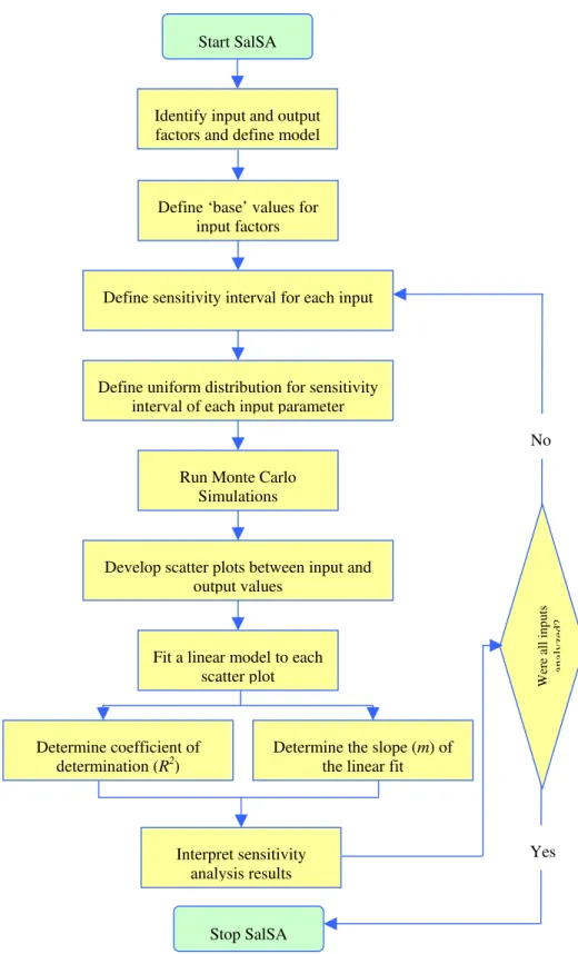
A new sensitivity analysis technique called, Simulation-based Localized Sensitivity Analysis (SaLSA) is proposed, which is a hybrid of the differential analysis and simulation-based sampling techniques. Figure 1 provides a flowchart that describes all the steps of the proposed technique.
In the following sections, we briefly describe the previously developed (Sadiq et al. 2007) Q-WARP model (Water Quality –Water mAin Renewal Planner) to predict water quality failures in the distribution networks. Subsequently we demonstrate the application of SaLSA to a case study analysis as applied in Q-WARP.
Start SalSA
Identify input and output factors and define model
Define ‘base’ values for input factors
Define sensitivity interval for each input
Define uniform distribution for sensitivity interval of each input parameter
Run Monte Carlo Simulations
Develop scatter plots between input and output values
Fit a linear model to each scatter plot
Determine the slope (m) of the linear fit
Stop SalSA Wer e all inputs analyzed? No Yes Determine coefficient of determination (R2) Interpret sensitivity analysis results
Sensitivity analysis – an example of water quality failures in distribution networks
Q-WARP
Various computational techniques may be appropriate to predict WQFs in aging water mains, but appropriateness of any technique depends on how readily it treats the uncertainties inherent in modelling and handle interacting concepts that encompass issues specific to water distribution networks. Fuzzy cognitive maps (FCMs), an extension of cognitive maps, are illustrative causative representation of complex systems (Kosko 1997). FCMs draw a causal representation among all identified factors of any specific system. A complex system represented by FCM can incorporate human experience, judgment, understanding and knowledge about the system. The FCM is a process model, which can use knowledge of expert opinion and belief (qualitative, soft) and/ or existing (quantitative, hard) data. FCM consists of nodes that represent factors involved in the system, and weighted arcs (connections), that represent causal relationships between factors. Arcs are graphically illustrated as signed weighted graphs with optional feedback loops. Factors can be inputs, outputs, variables, states, events, actions, goals, and trends of the system.
Q-WARP is a model based on hierarchical (two levels) FCMs. This model is used to predict the ‘potential’ (risk) for water quality failures in a given pipe segment. At the lower or modular level (or Level I), input factors related to pipe attributes, site-specific conditions, operational and hydraulic factors, water quality indicators, and decision actions are defined and used to quantify the potential for water quality deterioration due to different mechanisms including contaminant intrusion, internal corrosion, leaching, biofilm formation, disinfectant loss and THM formation, and permeation. In the supervisory level (or Level II), these deterioration mechanisms are assessed for their contributions to the potential for aesthetic, physico-chemical, microbiological and overall water quality failures (Figure 2).
Potential for contaminant intrusion
Po te nt ial fo r w a te r q u a lit y det e riorat ion mechani s
ms Potential for Internal corrosion
Potential for leaching
Potential for Biofilm formation
Potential for disinfectant loss and THMs formation
Potential for permeation
Modular FCMs (Level I)
Figure 2. Schematic representation of Q-WARP model
Physico-chemical
water quality failure
Microbiological
water quality failure
Aesthetic
water quality failure
⊕
Supervisory FCM (Level II)
Risk of water quality failures
⊕ ⊕
⊕
Potential for contaminant intrusion
Po te nt ial fo r w a te r q u a lit y det e riorat ion mechani s
ms Potential for Internal corrosion
Potential for leaching
Potential for Biofilm formation
Potential for disinfectant loss and THMs formation
Potential for permeation
Modular FCMs (Level I)
Physico-chemical
water quality failure
Microbiological
water quality failure
Aesthetic
water quality failure
⊕
Supervisory FCM (Level II)
Risk of water quality failures
⊕ ⊕
Q-WARP describes three types of water quality failures - aesthetic, physicochemical and microbiological. The overall risk of water quality failure is estimated based on these three types of water quality failure. Q-WARP considers approximately fifty factors, of which 25 are input factors that directly or indirectly influence water quality in distribution networks. All of these input factors feed into modular FCMs, whose outputs are used to stimulate the supervisory FCM. Many basic factors are common to more than one of the modular FCMs, e.g., pipe age, pipe diameter, etc., which leads to a strong interconnectivity between factors. This interconnectivity and redundancy of the factors in modular FCMs increase the complexity of estimating the contribution (sensitivity) of input factors.
Results and discussion
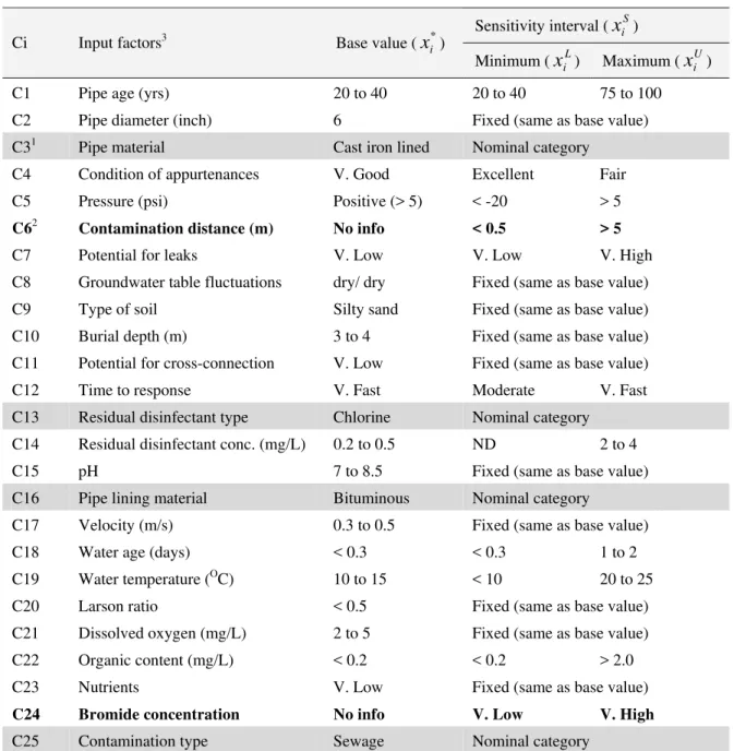
Consider a hypothetical pipe segment (any pipe length in which conditions are assumed homogenous) in a water distribution network, for which the potential for water quality failure needs to be determined. Data for the input factors are provided in Table 1. Note that although hypothetical, these data reflect realistic conditions. This data set represents instantaneous or average estimates for the input factors. Actual magnitudes (e.g., pressure, velocity, or other water quality indicators) may vary over time. Any representative value of these input factors can be analyzed.
Results of an example using the Q-WARP are provided in Figure 3, where potentials for the realization of various water quality deterioration mechanisms as well as water quality failures are shown. Three values, min, max and most likely, are provided for each prediction, using error bars. The interval [min, max] size is directly proportional to the amount of missing data. For example, the potential for intrusion has a wide range because the contributing factor contamination
distance is defined as ‘No info’ (i.e., missing data) in Table 1.
SalSA is implemented to evaluate the impacts of various input factors on water quality failures. Sensitivity is determined only for those factors, whose values can be mapped ordinally, e.g., pipe age, pipe diameter, velocity, etc. Non-ordinal (normative) input factors (e.g., pipe material (C3), pipe lining (C16), contamination type (C25), etc.) are set at pre-defined levels for a particular sensitivity analysis scenario. The sensitivity analysis in Q-WARP reports only relative rankings for each selected input factor based on their contribution to output.
The values of input factors in the simulations are assumed continuous in the selected sensitivity intervals. If ‘Full range’ is of interest then lower and upper ordinal values of the input factor become the min and max values of the sensitivity interval ( ). The can assume any interval within the full range of x
S i
x xiS
i (including a point, which means a ‘Fixed’ value). Those input factors
that are defined as ‘No info’, are treated by default as ‘Full range’.
Once sensitivity intervals (x ) are defined for the selected input factors, Monte Carlo iS
simulations are performed and the potential for water quality failures and potential for water quality deterioration mechanisms are calculated (a result of single iteration is similar to a snapshot shown in Figure 3). Sensitivity is determined for only those input factors for which sensitivity intervals ( ) are defined as non-point intervals or indicated as ‘No info’. The sensitivity analysis using SalSA has following pricipal features and characteristics:
S i
x
• Small sensitivity intervals ( ) for random sampling imply strong observational
interdependence among various input factors. Complete independence is approached if
sensitivity interval is large; S i
• The sensitivity of an input factor is determined based on a linear fit; therefore the larger sensitivity intervals ignore local perturbations;
• One-factor at a time (OFAAT) approach can be used to determine the sensitivity of a given input factor over its universe of discourse by keeping all other input factors ‘Fixed’ at any desired base value x*i , and a sensitivity profile can be established for that factor; and
• Results of the sensitivity analysis must be interpreted only relative to each other, i.e., used for ranking the input factors under a given scenario.
Table 1. Defining sensitivity interval (xiS) in the example
Sensitivity interval (xiS) Ci Input factors3 Base value (xi*)
Minimum (xiL) Maximum (xUi )
C1 Pipe age (yrs) 20 to 40 20 to 40 75 to 100
C2 Pipe diameter (inch) 6 Fixed (same as base value)
C31 Pipe material Cast iron lined Nominal category
C4 Condition of appurtenances V. Good Excellent Fair
C5 Pressure (psi) Positive (> 5) < -20 > 5
C62 Contamination distance (m) No info < 0.5 > 5
C7 Potential for leaks V. Low V. Low V. High
C8 Groundwater table fluctuations dry/ dry Fixed (same as base value)
C9 Type of soil Silty sand Fixed (same as base value)
C10 Burial depth (m) 3 to 4 Fixed (same as base value)
C11 Potential for cross-connection V. Low Fixed (same as base value)
C12 Time to response V. Fast Moderate V. Fast
C13 Residual disinfectant type Chlorine Nominal category C14 Residual disinfectant conc. (mg/L) 0.2 to 0.5 ND 2 to 4
C15 pH 7 to 8.5 Fixed (same as base value)
C16 Pipe lining material Bituminous Nominal category
C17 Velocity (m/s) 0.3 to 0.5 Fixed (same as base value)
C18 Water age (days) < 0.3 < 0.3 1 to 2
C19 Water temperature (OC) 10 to 15 < 10 20 to 25
C20 Larson ratio < 0.5 Fixed (same as base value)
C21 Dissolved oxygen (mg/L) 2 to 5 Fixed (same as base value)
C22 Organic content (mg/L) < 0.2 < 0.2 > 2.0
C23 Nutrients V. Low Fixed (same as base value)
C24 Bromide concentration No info V. Low V. High
C25 Contamination type Sewage Nominal category
1: shaded factors are nominal (non-ordinal) category
2: values of factors shown in bold letters were defined as ‘No info’ 3: sensitivity can be determined only for those factors that are not ‘Fixed’
0.09 0.28 0.37 0.31 0.0 0.2 0.4 0.6 0.8 1.0 A-WQF P-WQF M-WQF WQF Po te n ti a l
(b) Potential for water quality failures 0.29 0.00 0.00 0.25 0.25 0.00 0.10 0.0 0.2 0.4 0.6 0.8 1.0 PI PC PL PB PD PP PT Po te n tia l
(a) Potential for water quality deterioration mechanisms/ pathways
Figure 3. A snapshot of Q-WARP results
Data for two input factors, namely C6 (contamination distance) and C24 (Bromide
concentration), are assumed missing, therefore the sensitivity analysis of these factors is taken at ‘Full range’. The results of sensitivity analyses for 11 input factors are provided in Table 2 (based on sensitivity intervals described in Table 1). Sensitivity to potential for internal corrosion (PC) and potential for permeation (PP) are not shown, since the deterioration mechanisms are not relevant to 6” cement lined cast iron pipe. It can be noticed that potential for leaks (C7), time to response (C12) and condition of appurtenances (C4) were key factors in case of potential for intrusion (PI) under given conditions.
The results of sensitivity analysis require interpretation on relative scale (Table 2). Ranking is performed based on the absolute values (ignores positive or negative) of sensitivity results and provided in descending order. Table 2 provides a complete list of ranking orders for input factors for various output factors calculated based on their intensity. This ranking order of sensitivity is valid only for given conditions selected in the example as described earlier. For example, in case of potential for intrusion, the most sensitive factor was ‘potential for leaks’, and was assigned a rank of ‘1’ and so on. In this analysis, the ‘potential for cross-connection’ was assumed ‘fixed’ at a base value of very low, but the ranking order would have changed for all factors if it were allowed to vary, say, from very low to very high.
Table2. Ranking orders for the input factors based on sensitivity
Input factors * PI PL PB PT WQF
Pipe age (yrs) 3 2 3
Condition of appurtenances 2 2
Pressure (psi) 3 3
Contamination distance (m) 2 3
Potential for leaks 1** 2
Time to response*** 2 1
Residual disinfectant conc. (mg/L) 1 1 1 3
Water age (days) 1 1 2 3
Water temperature (OC) 2 3 3 3
Organic content (mg/L) 2 1 1
Bromide concentration 1 2
* Factors for which units are not provided were defined linguistically (e.g., low, medium, high). Smaller number represents higher severity of sensitivity and vice versa. PI: Potential for intrusion; PL: Potential for leaching; PB: Potential for biofilm formation; PT: Potential for THM formation; WQF: Overall water quality failures.
** Bold characters represent the most influential factor.
*** The contribution of an input factor to the overall WQF depends on multitude of interactions in modular FCMs. Therefore it is possible that in some cases the ranking order is lower in a specific water quality deterioration mechanism (modular FCM) and higher in overall WQF.
Summary
Water quality in a distribution network is a very complex system, affected directly or indirectly affect by numerous factors. These factors can be categorized as pipe attributes, site-specific factors hydraulics/ operational factors, water quality indicators and decision actions (or interventions). Interactions amongst these factors are very complex and often not well
understood. The modelling of complex dynamic systems requires methods that combine human knowledge and experience as well as expert judgment. Q-WARP (water Quality –Water mAin Renewal Planner) was developed in earlier work (Sadiq et al. 2007) to model complex system using fuzzy cognitive maps.
In this study, the contribution of impacts of input factors on complex system response is
investigated, using a newly developed technique called, Simulation-based Localized Sensitivity
Analysis (SaLSA), which is a hybrid of a differential analysis and simulation-based sampling techniques. The application of proposed technique SaLSA is demonstrated through the analysis of water quality failure as implemented in Q-WARP.
Acknowledgements
This paper presents interim results of a research project, which is co-sponsored by the AwwaRF, the NRC and water utilities from the United States and Canada. The authors wish to acknowledge
the invaluable help provided by Mr. Solomon Tesfamariam and Dr. Ahmed Abdel Akher at the NRC.
References
Frey, H.C., and Patil, S.R. 2002. Identification and review of sensitivity analysis methods, Risk Analysis, 22(3): 553-578
Hamby, D.M. 2004. A review of techniques for factor sensitivity analysis of environmental models,
Environmental Monitoring and Assessment, 32(2): 135-154
Helton, J.C., Johnson, J.D., Sallaberry, C.J., and Storlie, C.B. 2006. Survey of sampling-based methods for uncertainty and sensitivity analysis, Reliability Engineering and System Safety, 91(10-11): 1414-1434
Iman, R.L. and Helton, S.C. 1988. An investigation of uncertainty and sensitivity analysis techniques of computer models, Risk Analysis, 8(1): 71-90
Kleiner, Y. 1998. Risk factors in water distribution systems, British Columbia Water and Waste
Association 26th Annual Conference, Whistler, B.C., Canada
Koda, M., Dogru, A.H., and Seinfeld, J.H. 1979. Sensitivity analysis of partial differential equations with application to reaction and diffusion processes, Journal of Computational Physics, 30: 259–282
Kosko, B. 1997. Fuzzy Engineering, Upper Saddle River, NJ, Prentice Hall
Krieger, T.J., Durston, C., and Albright, D.C. 1977. Statistical determination of effective variables in sensitivity analysis, Transaction of American Nuclear Society, 28: 515–516
Makropoulos, C.K. and Butler, D. 2004. Spatial decisions under uncertainty: fuzzy inference in urban water management, Journal of Hydroinformatics, 6(1): 3-18
Ross, T. 2004. Fuzzy Logic with Engineering Applications, 2nd Edition, John Wiley & Sons, New York Sadiq, R., Kleiner, Y., and Rajani, B.B. 2004. Aggregative risk analysis for water quality failure in
distribution networks, AQUA - Journal of Water Supply: Research & Technology, 53(4): 241-261 Sadiq, R., Kleiner, Y., Rajani, B. 2007. A novel modelling approach to predict risk of water quality
failures in deteriorating water mains, pp. 223-228, Water Management Challenges in Global
Change CCWI2007 and SUWM2007 Conference, Edited by Ulanicki et al., Leicester, UK, Taylor and
Francis.
Salehi, F., Prasher, S.O., Amin, S., Madani, A., Jebelli, S.J., Ramaswamy, H.S. and Drury, C.T. 2000. Prediction of annual nitrate-n losses in drain outflows with artificial neural networks, Transactions of
the ASAE, 43(5): 1137-1143
US EPA 2001. Risk Assessment Guidance for Superfund: Volume III - Part A, Process for Conducting
Probabilistic Risk Assessment, U.S. Environmental Protection Agency, Washington D.C., EPA
540-R-02-002
US EPA 2007. US EPA White Papers, http://www.epa.gov/safewater/tcr/tcr.html, United States Environmental Protection Agency