HAL Id: hal-00316229
https://hal.archives-ouvertes.fr/hal-00316229
Submitted on 1 Jan 1996
HAL is a multi-disciplinary open access
archive for the deposit and dissemination of sci-entific research documents, whether they are pub-lished or not. The documents may come from teaching and research institutions in France or abroad, or from public or private research centers.
L’archive ouverte pluridisciplinaire HAL, est destinée au dépôt et à la diffusion de documents scientifiques de niveau recherche, publiés ou non, émanant des établissements d’enseignement et de recherche français ou étrangers, des laboratoires publics ou privés.
Time-dependent convection at high latitudes
D. W. Idenden, R. J. Moffett, S. Quegan, T. J. Fuller-Rowell
To cite this version:
D. W. Idenden, R. J. Moffett, S. Quegan, T. J. Fuller-Rowell. Time-dependent convection at high latitudes. Annales Geophysicae, European Geosciences Union, 1996, 14 (11), pp.1159-1169. �hal-00316229�
Ann. Geophysicae 14, 1159—1169 (1996) ( EGS — Springer-Verlag 1996
Time-dependent convection at high latitudes
D. W. Idenden1, R. J. Moffett1, S. Quegan1, T. J. Fuller-Rowell21 School of Mathematics and Statistics, The Hicks Building, University of Sheffield, Sheffield, S3 7RH, UK 2 CIRES, University of Colorado/NOAA Space Environment Laboratory, 325 Broadway, Boulder, CO 80303, USA Received: 12 January 1996/Revised: 20 May 1996/Accepted: 27 May 1996
Abstract. A fully time-dependent ionospheric convection model, in which electric potentials are derived by an analytic solution of Laplace’s equation, is described. This model has been developed to replace the empirically de-rived average convection patterns currently used routinely in the Sheffield/SEL/UCL coupled thermosphere/iono-sphere/plasmasphere model (CTIP) for modelling disturb-ed periods. Illustrative studies of such periods indicate that, for the electric field pulsation periods imposed, long-term averages of parameters such as Joule heating and plasma density have significantly different values in a time-dependent model compared to those derived under the same mean conditions in a steady-state model. These differences are indicative of the highly non-linear nature of the processes involved.
1 Introduction
The processes of magnetic field connection and reconnec-tion in the magnetosphere, first suggested by Dungey (1961), are now well established as the primary driving mechanisms for the two-cell convection pattern observed during periods of strong southward interplanetary mag-netic field (IMF). When the high velocity solar wind con-sisting of a hot magnetised plasma interacts with the magnetosphere, the whole system can be viewed as an enormous magnetohydrodynamic generator. A propor-tion of the large voltage (hundreds of kV) applied in the dawn-dusk direction across the magnetopause is mapped down into the ionosphere along highly conducting geomagnetic field lines when the latter become connected to the IMF, usually close to the subsolar point on the magnetopause. These connected, ‘open’ field lines have only one foot on the Earth and are swept into the tail of the magnetosphere by the solar wind. The electric field in
Correspondence to: D. W. Idenden
the ionosphere gives rise to an anti-sunward E]B drift across the polar cap which may be defined as the area enclosing these open field lines. Open field lines swept and stretched into the tail lobes will, at some stage, reconnect with their partners in the opposite hemisphere and return sunward under magnetic tension. These closed field lines map a dawn-dusk field into the ionosphere where the sunward convection is mirrored and a two-cell convection pattern arises.
Under steady-state conditions, snapshots of iono-spheric convection taken at different instants in time will be identical. Thus, the polar cap boundary separating anti-sunward convecting plasma on open field lines from sunward convecting plasma on closed field lines will re-main fixed. This condition implies that, since the magnetic flux is incompressible, plasma flowing into the polar cap through the dayside throat must be exactly balanced by the flow of plasma through the nightside exit region.
Most empirical models developed to describe iono-spheric convection are, by the nature of the method of their development, inherently steady-state. Such models make extensive use of satellite data (Heppner, 1977; Heppner and Maynard, 1987), radar data (Foster et al., 1986; Holt et al., 1987) or a combination of both (Heelis
et al., 1983). In addition, Friis Christensen et al. (1985)
describe how a global map of ionospheric convection is inferred from Greenland magnetometer data. Generally data is binned according to concurrent IMF conditions. Foster et al. (1986), however, bin their data according to the total amount of energy in precipitating particles infer-red from TIROS satellite measurements. Convection pat-terns are obtained for each dataset by a superposition and statistical averaging of many measurements spanning many hours, days or even months of observations. These models, then, should not be treated as snapshots of con-vection. The assumption that, at any given state of the solar wind field, a corresponding steady-state convection pattern prevails is most certainly flawed. In the event that the dayside and nightside merging rates do indeed depend only on the IMF conditions, there would nevertheless be an inevitable delay between the occurrence of a change in
the solar wind field at the dayside magnetopause and the transfer of such information many Earth radii into the tail of the magnetosphere where reconnection occurs. Lock-wood (1991) suggests that it may take in the region of 2 h of more or less constant IMF conditions to prevail before steady-state convection is achieved. Such events are rare, occurring only 15% of the time (Rostoker et al., 1988). Additional complications arise in the form of substorms whereby solar wind energy is stored in the magnetotail and released explosively.
Thus, in general, empirical models and their analytical fits (for example Hairston and Heelis, 1990) must be re-garded as average convection patterns. A snapshot of the instantaneous pattern may look very different from these empirical models and even gross mean features may be lost by the smearing effect of the statistical averaging process. Holt et al. (1987) report the loss of such large features as the Harang discontinuity which is clearly seen on individual days but disappears in averages over large data sets. The recent analysis procedure, AMIE (Rich-mond, 1992) has gone some way to solving this problem. The technique involves performing a least squares fit of an analytic electric potential distribution to data obtained simultaneously by many different instruments (i.e. satellite, magnetometer and radar), though some assumptions re-garding ionospheric conductivity need to be made in order to obtain electric fields from the derived current system.
The model described in this study is based on an analytic solution of Laplace’s equation on a plane surface which was originally solved for non-steady-state recon-nection by Siscoe and Huang (1985) who imposed bound-ary conditions by specifying the potential around the polar cap boundary only. Flux is considered to enter and leave the polar cap through only the throat and night exit regions respectively. The throat maps to the merging line at the dayside magnetopause where connection to the IMF occurs, while the night exit maps to the region where field lines close in the neutral sheet. The remainder of the polar cap boundary is considered adiaroic, i.e., no plasma may flow across it.
Siscoe and Huang’s solution was restricted to dayside merging only. Thus, the polar cap expanded continuously as plasma flowed through the throat. Our model repre-sents an improvement over the Siscoe and Huang formu-lation in a number of respects: (1) both dayside and nightside merging may be simulated; (2) the latitudinal extent of convection may be restricted by imposing a sec-ond boundary beysec-ond which the electric potential falls to zero. Such a restriction enables better fits to be obtained to empirical models such as those of Heppner and Maynard (1987) and Foster et al. (1986) and takes better account of theoretical arguments which invoke shielding by the ring current to prevent penetration of the electric field to lower latitudes (for example Wolf, 1975); (3) dawn-dusk asymmetries may be produced by (a) placing throat and exit regions asymmetrically and (b) adding a mono-pole term (which has only a radial electric field component and thus adds a vortex component to the flow lines) to the solution. These refinements allow for the possibility of extending the model to allow for flows observed when the
By component of the IMF is non-zero.
In using a solution of Laplace’s equation with the type of boundary conditions we have described, we have essen-tially made two implicit assumptions; (1) that the conduc-tivities are uniform within the area of interest and (2) that field aligned currents are restricted to the polar cap and zero potential boundaries only. While the first assumption is evidently not true, Moses et al. (1994) found that plasma flows during a geomagnetic storm could be modelled more accurately by assuming uniform conductivity than by imposing a highly conducting auroral oval or day/ night conductivity gradient. The effect of the former would only be significant near to the throat and night exit regions (the only regions where there is communication between polar cap and auroral plasma). In these areas flow lines would be kinked while gradients across the terminator tend to concentrate flow lines in the dawn sector. Nevertheless the two cell convection pattern per-sists for strongly southward IMF. Iijima and Potemra (1978) showed that large-scale region 1 and region 2 cur-rent systems were restricted to the poleward and equator-ward edge of the field aligned current region in the auroral oval at all magnetic local time sectors apart from a few hours pre-midnight where current regions overlap in a more complex fashion. Thus, although indeed the ma-jority of current flows along the surface of two concentric cylinders, there are significant field aligned currents across much of the auroral ionosphere. The justification for our approach here is that the flow patterns we obtain under steady-state conditions agree well with average empirical models.
Numerical solutions to Laplace’s equation have also been developed by Moses et al. (1987, 1989). Boundary conditions are set along a spiral polar cap boundary which allows modelling of large zonal flows near the merging gaps of the types observed during periods when the magnitude of the IMF By component is large. While no direct observational evidence would suggest a spiral shape for the polar cap boundary, good fits to many single pass satellite measurements during a geomagnetic storm have been obtained with this model (Moses et al., 1994).
2 Model description
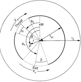
Assuming that ionospheric currents perturb the Earth’s magnetic field only slightly, we can take +]E"0 and hence define the electric field E by a scalar potential U where, by convention, E"!+U. For the purpose of describing the analytic electric field model, we need first to define a coordinate system whose origin is at the centre of the polar cap (Fig. 1). The model electric potentials are those that will give the desired E]B velocities when measured in the rest frame of this system. Azimuth is measured anti-clockwise from the meridian that passes through the geomagnetic pole while r is measured from the coordinate origin. Following Siscoe and Huang (1985), the potential must first be specified around the polar cap boundary. In the steady-state case, the adiaroic segments of the boundary are equipotentials while the potential varies linearly along them when merging is unbalanced. Dayside and nightside merging rates are controlled by
Fig. 1. The geometry of the polar cap. The geopotential coordinates (/, r) are shown for the point P. The geopotential pole is at the centre of the polar cap, and the geomagnetic pole is marked M. The bold lines mark the adiaroic sections of the polar cap boundary. The outer boundary shows the extent of the high-latitude convection pattern./d and /n are the azimuths of the centre of the throat and night exit regions respectively which have half-widths of a and b respectively. »d and »n are the voltages measured across the two gaps
specifying the potential differences across the throat and night exit regions, »d and »n, respectively. Any difference between »d and »n is distributed uniformly around the adiaroic boundary segments. The potential in the flux gaps takes the form:
U (r"rpc, /)"a
A
/!/0aB
#bA
/!/0 aB
3
#c, (1)
where a is the flux gap half-width, rpc is the polar cap radius, /0 is the azimuth of the centre of the flux gap (equal to /d and /n for the dayside and nightside gaps respectively), and a, b and c are calculated to obtain the required potential drop across the gap and uniformity in LU/L/ around the boundary. The coefficient c is required for flux gaps positioned asymmetrically on the boundary, though it may arbitrarily be set to zero for either one of the gaps. The general solution of Laplace’s equation may be written: U (r, /)"+= n/1
A
r aB
n(An cos(n/)#Bn sin(n/)) #+= n/1
A
r aB
~n (Cn cos(n/)#Dn sin(n/)) #E ln (r)#F. (2)The coefficients, An, Bn, Cn, and Dn, may be obtained by imposing the conditions at the polar cap boundary and at the zero potential boundary. E ln (r) is the term referred to previously as the monopole term. The Fourier coefficients
for the potential along the polar cap boundary are given by: an"1n2n: 0 sin (n/) U(r"rpc, /)d/ (3) and bn"1n 2n : 0 cos (n/) U(r"rpc, /)d/. (4) The solution now takes different forms in the three regions
r(rpc, rpc(r(r0 and r'r0 where r0 is the radius at
which the potential falls to zero.
2.1 In the auroral oval, rpc(r(r0
Continuity in the potential at the polar cap implies the conditions
An#Cn"an (5)
and
Bn#Dn"bn. (6)
Additionally, the boundary conditionU(r0)"0 requires that
A
r0 rpcB
n An#A
rpcr0B
~nCn"0 (7) andA
r0 rpcB
n Bn#A
rpcr0B
~nDn"0 (8) are satisfied for all n. Thus, solving for the unknowns An,Bn, Cn and Dn in Eqs. (5—8) gives An" an 1!
A
r0 rpcB
2n, (9) Bn" bn 1!A
r0 rpcB
2n, (10) Cn" an 1!A
rpc r0B
2n, (11) Dn" bn 1!A
rpc r0B
2n. (12)E may be chosen to fit data or empirical models and F can
be adjusted to ensure that the condition U(r0)"0 is satisfied:
F"!E ln
A
r0Fig. 2a–c. Plots of equipotentials (plasma flow lines). Arrows indi-cate flow direction. a Steady-state convection in the corotating frame; b steady-state convection in the Sun-fixed (non-corotating) geomagnetic frame; c as b, but omitting correction to boundary potential to force the boundary to be stationary in this frame. Flow is seen across adiaroic boundary segments (bold lines). The dot-dashed line marks the extent of the high-latitude convection pattern. Noon MLT is at the top of these plots
2.2 Inside the polar cap, r(rpc
The requirement that the electric potential be finite within the polar cap, and in particular at the origin, allows us to drop many of the terms in Eq. (2):
C@n"D@n"E@n"0, (14) where @ denotes the area inside the polar cap boundary. Thus, within the polar cap, the potential is given by: U(r, /)"+= n/1
A
r aB
n (A@ncos(n/)#B@nsin(n/))#F@. (15) Continuity inU at the boundary enables us to determine the remaining coefficients:A@n"an, (16)
B@n"bn, (17)
F@"F. (18)
2.3 Outside the high-latitude region, r'r0
The magnetospheric potential is set to zero at all points. The dynamo effect generates electric fields at lower lati-tudes. These are not considered here.
3 Correction for corotation
The electric field model described so far enables a two-cell convection pattern to be generated in the corotating frame as measured by an Earth-bound observer or after trans-formation of satellite measurements by removing the corotation velocity. The underlying assumption in defin-ing the potential along the polar cap boundary, essentially the boundary conditions used to solve Laplace’s equation, is that the polar cap boundary is stationary in the corotat-ing frame (and thus an equipotential under steady-state conditions). However, results obtained by fitting circular convection reversal boundaries to potential extrema from satellite observations (Meng et al., 1977; Hairston and Heelis, 1990) would indicate that the centre of the polar cap is displaced a few degrees to the nightside of the geomagnetic pole. These observations are also confirmed by fitting convection reversal boundaries to the empirical models of Foster et al. (1986) which are described later in this study. Thus, the polar cap boundary is stationary in the sun-fixed geomagnetic frame (i.e. that defined by MLT and invariant latitude). The boundary conditions we have described i.e. an equipotential under steady-state condi-tions or linearly varying for an expanding/contracting polar cap are relevant to this frame. To obtain the poten-tial function along the boundary in the corotating frame, we must make a correction by subtracting the ‘corotation potential function’, UMC, which describes the motion of corotating plasma in the Sun-fixed geomagnetic frame. Quegan et al. (1986) showedUmc to depend on invariant latitude and UT only, the UT dependence arising from the offset of the geomagnetic and geographic poles. The corota-tion potential measured around the boundary is a cosine .
Fig. 3a–c. Snapshots of equipotential plasma flow lines in the Sun-fixed geomagnetic frame. a Expanding polar cap convection pat-tern; b contracting polar cap; c steady-state convection pattern with By-type flows: circulation within the polar cap and asymmetric dawn/dusk cells. Noon MLT is at the top of these plots
function of azimuth measured in the geopotential coordi-nate system plus a constant offset potential. The offset may be ignored since it is only the potential gradient which is of interest for plasma dynamics. Thus,
Umc(/, r"rpc, UT)"Ac(rpc, UT)cos/. (19) The amplitude of the corotation potential around the boundary is given by:
Ac(rpc, UT)"kcos(hm)!sin(d)sin(d@)1!sin2(d)
]
C
sin2(rpc!hp)!sin2(rpc#hp)2
D
, (20) wherehm is the separation of the geomagnetic and geo-graphic poles,hp is the separation of the geomagnetic pole and the polar cap centre,d and d@ are the Sun’s declina-tions in the geographic and Sun-fixed geomagnetic frames respectively (the latter being implicitly UT dependent), and k+!84543 V. Now it is a straightforward matter to subtract the corotation potential from the boundary by adjusting the first cosine Fourier coefficient,a1:a1"a@1!Ac(rpc, UT), (21) wherea@1 is the coefficient obtained in the geopotentialrest frame.
Figure 2a shows an example of the resulting steady-state convection pattern in the corotating frame. The adiaroic boundary is no longer an equipotential since the boundary itself is moving in this frame. Figure 2b shows the same pattern in the Sun-fixed geomagnetic frame in which the boundary is stationary and thus an equipoten-tial. This may be contrasted with Fig. 2c in which no correction term has been included in the electric field and consequently flow lines can be seen passing through the stationary ‘adiaroic’ boundary segments. Figure 3a, b shows typical non-steady-state convection patterns with the inclusion of the correction term for expanding and contracting polar caps respectively.
4 Non-zero Byfields — a possible extension to the model
The model described so far is considered to present a sig-nificant improvement over the analytic model described by Siscoe and Huang (1985) and thus, an appropriate starting place in time dependent modelling of the high-latitude ionosphere/thermosphere system in a self-consis-tent regime. Nevertheless, flows resulting from a non-zero
By component of the IMF have not been included in the
model, though these are considered briefly below where we suggest ways in which they might be incorporated into the analytic field.
Non-zero By fields are characterised by a number of features in the ionospheric flow paths which arise from field line tension and may be summarised for the Northern Hemisphere as follows:
a. The dayside cusp is displaced toward dusk (dawn) for positive (negative) By (Lockwood et al., 1990; Reiff and Burch, 1985).
b. The convection cells become asymmetric. For posi-tive (negaposi-tive) By, the dawn (dusk) cell is kidney-shaped and partially surrounds the larger dusk (dawn) cell. The electric field and hence convection is enhanced on the dawn (dusk) side.
c. The geometry described results in strong zonal flows within the polar cap which are westward (eastward) for
positive (negative) By. Moses et al. (1987, 1989) model
By flows using a numerical scheme for solving Laplace’s
equation with a spiral polar cap boundary. In the analytic model described here, a number of refinements can be added to simulate such flows: (a) the position of the day-side throat can be moved duskward/dawnward depending on the required value of By; (b) the monopole term affect-ing flows outside the boundary may be adjusted to pro-duce kidney shaped convection cells; (c) within the polar cap, a circulation term may be added to produce zonal flows as suggested by Siscoe and Huang (1985). A circula-tion term which by itself would produce flow of constant angular velocity around the polar cap (similar to the way in which the corotation potential produces flow around the geographic poles in the Sun-fixed frame) is not actual-ly a solution to Laplace’s equation and would therefore require a continuous distribution of field-aligned Birke-land currents to support it.
The effect of these refinements is shown in Fig. 3c. When the circulation term is of similar magnitude to the cross polar cap potential drop, a lobe cell is formed within the polar cap which has been observed during weak southward Bz and strong By (Reiff and Burch, 1985). Such flows are attributed to lobe stirring due to reconnection of already open field lines with the interplanetary magnetic field (Crooker, 1979). During periods of northward IMF when dayside merging disappears altogether, flows will be dominated by this lobe stirring, nightside reconnection and viscous flow.
5 Model summary
The model described uses an analytic solution of Laplace’s equation on a two-dimensional plane and is a good approximation to a solution on a spherical surface for latitudes close to the poles. The model requires as inputs: the initial polar cap radius; the voltages across the dayside and nightside merging gaps, each as functions of time; the throat and exit widths and positions on the polar cap boundary (also functions of time); and the magnitude of the monopole term. While some dawn-dusk asymmetry is permitted in the flow by moving the positions of the merging gaps, and including a monopole term outside the polar cap, these adjustments are at present used only to obtain better fits to empirical models. We suggest means by which non-zero By flows may be modelled in the analytic framework.
6 Effect on the ionosphere of time-dependent convection
To test the effects of time varying electric fields on the high-latitude ionosphere, the time-dependent convection model has been incorporated into the Sheffield/SEL/UCL coupled thermosphere/ionosphere/plasmasphere model (CTIP).
6.1 Incorporating time-dependent convection into CTIP
The time-dependent convection model has replaced the empirical model of Foster et al. (1986) in a development version of the CTIP (Millward et al., 1995) with the intention of: (1) comparing average results obtained using time varying electric fields with those from a steady-state field to determine the shortcomings of steady-state models in predicting mean values of ionospheric and thermo-spheric parameters; (2) looking for transient effects pro-duced by pulsed electric fields.
The empirical models of Foster are matched to maps of precipitation determined by the TIROS-NOAA satellites (Fuller-Rowell and Evans, 1987), each parametrised by an index denoting the mean power of precipitation. Appro-priate steady-state conditions for the present model were determined by fits to the electric fields obtained from the Foster empirical model at each precipitation level. Fits were obtained by a least squares method in which the position of the polar cap centre, polar cap radius, zero potential radius (r0), position of merging gaps, monopole amplitude and cross-polar-cap voltage were optimised. Constraints on fits were that the dayside and nightside potential differences remained equal (the condition of steady-state) and the widths of the merging gaps remained at 90°. Relaxation of this latter condition results in the gaps growing much larger. This is due to the rotational shears apparent around much of the polar cap boundary in the empirical models. Such flows may, in part, arise from viscous flows which would produce rotational shears around the whole polar cap boundary but are not con-sidered by our model. Apparent rotational shears may also be generated in empirical models derived by aver-aging over periods when the polar cap is expanding and contracting over its mean location (Lockwood, 1991). Additionally, radars employing beam swinging techniques may measure rotational reversals where shear reversals actually exist due to assumptions of spatial uniformity of flow employed to make such measurements (Lockwood
et al., 1988). Single-pass satellite measurements do,
how-ever, tend to show shear reversal on large sections of the polar cap boundary, implying the presence of adiaroic segments and confined throat and night exit regions (Heelis et al., 1976, 1982, Heelis and Hanson, 1980). Plots of equipotentials for the empirical models are shown in Fig. 4 along with the fits for the present model for precipi-tation levels 5 and 9.
6.2 Dealing with precipitation in time-varying convection
Precipitation during time-varying conditions has been calculated using the TIROS-NOAA precipitation patterns corresponding to the mean conditions during the period. The pattern as a whole is simply made to expand or contract in proportion to the radius of the polar cap. Such a time-varying precipitation model is used as a first attempt in the absence of appropriate empirical models.
Fig. 4a–d. Plasma flow line equipoten-tials in the Sun-fixed geomagnetic frame for the Foster et al. (1986) model, a and c and the time- dependent model dis-cussed in this work fitted to the Foster et al. (1986) model, b and d. a and b are for activity level 5, and c and d are for activity level 9. Noon MLT is at the top of these plots, and contours are at intervals of 2 kV
7 Time-dependent and steady-state computations
A comparison of results obtained using steady-state and time-dependent models with the same mean conditions (cross-polar-cap voltage, »pc, and polar cap area) has been undertaken to determine the effect of non-steady convec-tion on average values of thermospheric and ionospheric parameters and thus the limitations of steady-state models in determining accurate values of these parameters. In this context, »pc is defined as the dawn-dusk potential drop across the polar cap measured along any line which passes through the centre of the polar cap and intersects the adiaroic boundary in both the morning and afternoon sectors.
Both versions of CTIP were run for 24-h simulations to reach quasi-steady states before average values were ob-tained for parameters over a 1-h period for the area close to the northern polar cap. Three days contrasting greatly in plasma density distribution were chosen for study: winter solstice (day 355), summer solstice (172) and north-ern autumn equinox (263). Comparisons were made for both quiet-time mean conditions corresponding to activ-ity level 5 (KP"2#, »pc"29 kV) and more disturbed conditions, activity level 9 (KP"5!, »pc"66 kV).Time dependent electric fields are modelled by a polar cap expansion phase followed by a contraction about the desired mean polar cap area with a 1-h period. During
expansion, the nightside flux gap width and voltage are both set to zero, and the dayside voltage set to obtain the same polar cap voltage, »pc, (as defined already) as in the steady state case (»SS). Since the potential varies linearly along the adiaroic boundary segment, which in this in-stance is 270° in azimuthal extent, this latter requirement is satisfied by setting »d"32»SS. Similarly during contrac-tion the dayside voltage and flux gap widths are set to zero, and »n"32»SS. Thus, dayside and nightside voltages have square wave forms and are 180° out of phase with each other. Although somewhat arbitrary, these condi-tions do ensure that the plasma velocity through the exit region is never less than the boundary velocity. If this were not the case, previously closed flux tubes on the nightside could effectively become open, which is un-physical. The 1-h period is chosen as roughly the time scale for substorm activity. Though results obtained using other periods will not be presented here, preliminary examination of par-ameters obtained using a 0.5-h period did not reveal any significant (i.e greater than a few percent) differences to those obtained with the 1-h period. The polar cap radius is calculated self-consistently at each time step according to the rate of expansion/contraction due to the electric field along the adiaroic boundary segment.
Particular emphasis was placed on the study of Joule heating which is the primary mechanism by which energy is dissipated in the neutral atmosphere by convection.
c
Fig. 5a–c. Rate of energy input to the F-region (pressure level 12) thermosphere averaged over a 1-h period measured in W kg~1. a Steady-state, b time-varying for the same mean conditions as a, c the additional heating due to time-varying field over steady-state. The position of the polar cap boundary (solid and dashed circle) and the continents is shown midway through this period (12.5 UT). Noon local time is at the top of the plots. The colour scale shown by the upper bar is for plots a and b and the lower bar is for plot c Table 1. Comparison of steady-state (SS) and time-dependent (TD) mean Joule heating rates for the high-latitude Northern Hemisphere region, pressure level 12 (approx. 280 km), W kg~1. Values are shown for two regions, the polar cap (r(rpc) and the annulus between the polar cap boundary and zero potential boundary (rpc(r(r0), two activity levels and three days.
Day number r(rpc rpc(r(r0
Activity Activity Activity Activity level 5 level 9 level 5 level 9 355 SS 5.12 14.8 10.1 22.5 TD 11.2 29.5 13.2 35.7 172 SS 5.98 7.32 12.7 16.9 TD 9.01 13.1 14.6 22.2 263 SS 7.52 13.9 13.9 21.2 TD 14.7 26.1 17.7 33.0
Complementary to this was the study of plasma densities which both influence Joule heating (since this depends directly on ionospheric conductivity), and are influenced by frictional heating of the ionosphere (equivalent to Joule heating) which can cause plasma depletion via temper-ature dependent loss reactions. Plasma convection also couples to the thermosphere via electrodynamic (Lorentz) forcing which results in momentum transfer to the neutral atmosphere giving rise to large-scale neutral winds. Neutral winds are also generated by thermal expansion of the thermosphere produced by Joule heating. These winds may have a component perpendicular to the Lorentz force which is predominantly in the direction of ion flow in the F region. We report here a sample of our results for the Northern Hemisphere as illustrations of the effects of time dependent convection.
7.1 Results
Values for the time- and area-averaged rates of energy input by Joule heating into the thermosphere within the boundary defining the latitudinal extent of the high-lati-tude magnetospheric convection at F-region heights (pres-sure level 12, about 280 km) have been calculated for steady-state and time-dependent models. These values are shown in Table 1. The largest difference is seen for the lower activity level at winter solstice when the time vary-ing field produces nearly 120% more heatvary-ing within the polar cap than the steady-state field. Joule heating en-hancements of at least 80% within the polar cap are seen in all other datasets apart from during the lower activity level at summer solstice when this value is only 50%. Enhancements in the annulus outside the polar cap are significantly less than inside the polar cap. At the lower
Table 2. Comparison of steady-state (SS) and time-dependent (TD) total Joule heating rates for the high-latitude Northern Hemisphere region within the zero potential boundary above 120 km altitude (GW). Values are shown for two activity levels and 3 days Day number Activity Activity
level 5 level 9 355 SS 5.92 53.1 TD 7.97 71.8 172 SS 12.3 73.1 TD 16.6 110.5 263 SS 8.25 61.0 TD 10.2 86.2
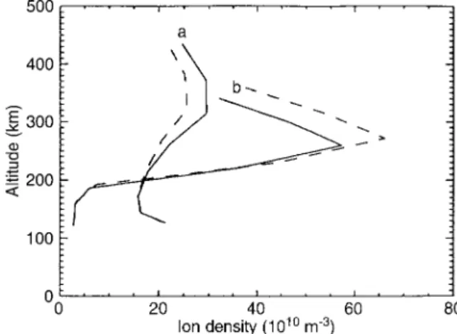
Fig. 6. Mean ion density profiles for the polar cap at summer solstice and high activity level a and winter solstice and low activity level, b. Dashed lines are for time-varying conditions and solid lines for steady-state conditions
activity level during the northern winter solstice the differ-ence in heating rates is only 30% in the annulus, while the largest difference (59%) in this region is seen at the same time of year but at the higher activity level.
The polar plots in Fig. 5a, b show the mean power dissipated over a 1-h period for the steady-state and time-dependent models respectively, for the lower activity level at winter solstice, while Fig. 5c displays the difference in these two values. Similar plots obtained for the other periods and activity levels show qualitatively the same gross features, indicating that, for both models, most Joule heating occurs near the flux gaps and particularly at the gap edges where ion velocities are very large and the flow characterised by rotational shears. The greatest differ-ences in the two models also occur at the flux gap edges where the time-varying field causes greater heating. Differ-ences are much less in the regions between the polar cap and the zero potential boundary. This appears to be due to there actually being less energy input in the time-depen-dent model than in the steady-state model in the sectors between the adiaroic boundary segments and the fixed zero potential boundary. This difference may result from the fact that, during time-dependent convection, the polar cap expands and contracts about a mean area equal to that in the steady-state case. This means that the mean radius of the polar cap is actually less in the time-depen-dent case, the separation of the polar cap boundary and zero potential boundary is greater and thus the mean electric fields in this region are reduced.
Volume integrated Joule heating values have also been obtained for the two models for the region inside the zero potential boundary at altitudes above 120 km. These values are shown in Table 2 and indicate that time-depen-dent convection would generally be responsible for an additional 25—50% energy input into this region of the atmosphere.
Comparison of ion density profiles averaged over the polar cap area for the lower activity level (Fig. 6) shows the trend for ion density to increase for the time-depen-dent model with peak values being some 20% larger at winter solstice than in the steady-state model. This differ-ence is less at other times, being negligible at summer solstice. This trend is reversed for the higher activity level with a time-varying field reducing ion densities. For both activity levels, however, the effective temperature (which is a function of the ion and nitrogen temperatures and
rela-tive ion-neutral velocity) is increased with a time-varying electric field. Both these results may be explained by considering the rate coefficient, k1, for the main plasma loss process at F-region altitudes:
O`#N2PN#NO`. (22)
The rate, k1, is dependent on the effective temperature and has a minimum value at a temperature of 1050 K. It increases markedly for temperatures greater than this value (St. Maurice and Torr, 1978). In the winter at the lower activity level effective temperatures are generally well below the loss rate minimum. Thus the increase in effective temperature resulting from increased R.M.S. ion-neutral relative velocities due to time varying electric fields actually reduces the plasma loss rate. For the lower activity level at summer solstice temperatures are close to, or slightly above, the threshold leaving the ion densities very nearly unchanged in a time-varying field, while at the higher activity level, increased ion temperatures result in increased losses and plasma depletion.
Increased Joule heating observed during time-varying convection results in localised heating of the neutral atmosphere. Transport of heat away from these localised areas means that the mean heights of all pressure levels are increased for the whole of the area defined by the extent of the high-latitude ionospheric convection pattern. It has been found (results not shown) that the mean height increase varies between 1 km at 120 km altitude and 20 km at 400 km altitude.
Also important in coupling the ionosphere to the neu-tral atmosphere is momentum transfer whereby plasma drift significantly alters neutral winds. In fact, at F-region altitudes and high latitudes this is the main process by which thermospheric winds are generated. The important mechanism in this respect is that of ion drag (or equiva-lently electrodynamic forcing). However, pressure differ-ences at fixed heights generated by Joule heating of the atmosphere as described will result in additional horizontal thermospheric winds and increase the momentum transfer of ionospheric convection to the neutral atmosphere.
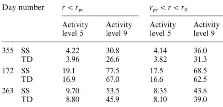
Table 3. Comparison of steady state (SS) and time-dependent (TD) values of total translational kinetic energy of the neutral air wind (1012J). Values are shown for two regions in the Northern Hemi-sphere, the polar cap (r(rpc) and the annulus between the polar cap boundary and zero potential boundary (rpc(r(r0), two activity levels and 3 days.
Day number r(rpc rpc(r(r0
Activity Activity Activity Activity level 5 level 9 level 5 level 9 355 SS 4.22 30.8 4.14 36.0 TD 3.96 26.6 3.82 31.3 172 SS 19.1 77.5 17.5 68.5 TD 16.9 67.0 16.6 62.5 263 SS 9.70 53.5 8.35 43.8 TD 8.80 45.9 8.10 39.0
As a measure of the momentum transfer to the thermo-sphere, the total translational kinetic energy of the neutral winds above a height of 120 km has been calculated for the two models. These values are shown for comparison in Table 3 for the area inside the polar cap and the annulus between the polar cap boundary and latitude of zero potential. It needs to be emphasised that these winds are not generated by ionospheric drifts alone, and have con-tributions from thermal winds which would exist in the absence of ionospheric drifts. In places where drift gener-ated winds oppose thermal winds, the former will actually reduce neutral kinetic energy. Thermospheric winds are also generated by the upwards propagation of tidal effects which are imposed at an altitude of approximately 100 km in the coupled model. These tides are the same in the time-dependent and steady-state models. Therefore, although absolute values for the total wind energy will depend on the height above which we integrate, we would neverthe-less expect the differences in results for the two models to be qualitatively the same regardless of the exact integra-tion heights. Significant differences are indeed seen be-tween the steady-state and time-dependent model results which must be related to momentum transfer processes. It is seen that the total kinetic energy of the neutral atmo-sphere is actually reduced in time-varying convection on all 3 days studied and for both activity levels. The differ-ence is greatest for the higher activity level where ion drag forces will dominate neutral atmosphere dynamics. For the higher activity level, the reduction in neutral winds is not unexpected since time-varying fields have been shown to reduce ion concentrations which in turn reduces the ion drag force on the neutrals. Conversely, one might expect the increase in ion concentrations at the lower activity level to actually increase ion drag. However, an explana-tion can be obtained for the reducexplana-tion in neutral gas velocities by considering effects close to an adiaroic section of the polar cap boundary during time-dependent convec-tion. A parcel of neutral gas which is stationary at this point will experience the passage of plasma which be-comes anti-sunward as the polar cap boundary expands over its location. Some time later, the boundary will contract, so that the parcel lies outside the boundary and
experiences plasma flow which is sunward. The neutral gas has a response time to the ion drag force which is longer than the polar cap cycle period, and thus will respond roughly to the time-averaged ion velocity in this case. It can be seen from this argument that the time averaged ion velocities, and thus the neutral velocities, in the region bounded by the extrema in boundary locations during the time-dependent case will be reduced compared to the steady-state case, this effect being greatest close to the mean location of the polar cap boundary.
8 Summary
We have described a fully time-dependent high-latitude ionospheric convection model based on a solution of Laplace’s equation. The model allows for an expanding and contracting polar cap boundary which encloses open anti-sunward convecting field lines. The model described has been successfully incorporated into the Sheffield/ UCL/SEL coupled thermosphere/ionosphere/ plasma-sphere model and results compared with those obtained with average steady-state conditions. Future improve-ments to this model will be the inclusion of non-zero
By-type flows and flows generated by viscous interaction
of the solar wind with plasma on closed field lines. In the simplified treatment described here, precipitation patterns used in the coupled model have simply been scaled in spatial extent during expansion and contraction of the polar cap. More sophisticated time-dependent precipita-tion models will obviously be required for more detailed quantitative studies of disturbed periods.
The comparisons of steady-state and 1-h time-varying field results for the northern polar cap region may be summarised as follows:
1. At F-region altitudes, the time-dependent model produces enhanced Joule heating compared to the steady-state model inside the polar cap. These enhancements are largest (120%) for quiet conditions at winter solstice. In regions close to flux gap edges, this value rises to nearly 150%. The total (volume integrated) increase in energy input to the region of the atmosphere above 120 km inside the zero potential boundary is generally about 35%. Dur-ing summer solstice at activity level 9 (Kp"5!) this value rises to 50%. Thus, steady-state models may signifi-cantly underestimate an important energy source in the high-latitude ionosphere.
2. Momentum transfer to the thermosphere is slightly reduced when time variability is taken into account, with total translational kinetic energy of the neutral winds decreasing by about 10% at altitudes above 120 km. This decrease is due in part to the reduction in the mean ion velocities close to the mean location of the adiaroic boundary sections of the polar cap. This results from the alternating passage of anti-sunward- and sunward-con-vecting plasma as the polar cap expands and contracts about its mean location.
3. Of all the parameters studied, changes in ion densi-ties are the most dependent on the chosen conditions. During quiet winter time conditions the average polar cap density at the F2 peak actually increases by some
20% during time-varying conditions due to a decrease in plasma loss rates. Conversely when effective ion temperatures are generally higher, for example during summer and in more disturbed periods, time-varying con-vection reduces average ion density by about 15%.
Acknowledgements. This work has been supported by PPARC under grant GR/K 06112. We thank R. A. Heelis for helpful discussions.
Topical Editor D. Alcayde´ thanks A. D. Richmond and G. Rostoker for their help in evaluating this paper.
References
Crooker, N. U., Dayside merging and cusp geometry, J. Geophys. Res., 84, 951—959, 1979.
Dungey, J. W., Interplanetary magnetic field and the auroral zones, Phys. Rev. ¸ett., 6, 47—48, 1961.
Foster, J. C., J. M. Holt, R. G, Musgrove, and D. S. Evans, Iono-spheric convection associated with discrete levels of particle precipitation, Geophys. Res. ¸ett., 13, 656—659, 1986.
Friis Christensen, E., Y. Kamide, A. D. Richmond, and S. Matsushita, Interplanetary magnetic field control of high-latitude electric fields and currents determined from Greenland magnetometer data, J. Geophys. Res., 90, 1325—1338, 1985.
Fuller-Rowell, T. J., and D. S. Evans, Height-integrated Pedersen and Hall conductivity patterns inferred from the TIROS-NOAA satellite data, J. Geophys. Res., 92, 7606—7618, 1987.
Hairston, M. R., and R. A. Heelis, Model of the high-latitude ionospheric convection pattern during southward interplanetary magnetic field using DE 2 data, J. Geophys. Res., 95, 2333—2343, 1990.
Heelis, R. A., and W. B. Hanson, High-latitude ion convection in the night-time F region, J. Geophys. Res., 85, 1995—2002, 1980. Heelis, R. A., W. B. Hanson, and J. L. Burch, Ion convection
reversals in the dayside cleft, J. Geophys. Res., 81, 3803—3809, 1976.
Heelis, R. A., J. K. Lowell, and R. W. Spiro, A model of the high-latitude ionospheric convection pattern, J. Geophys. Res., 87, 6339—6345, 1982.
Heelis, R. A., J. C. Foster, O. de la Beaujardiere, and J. Holt, Multistation measurements of high-latitude ionospheric convec-tion, J. Geophys. Res., 88, 10111—10121, 1983.
Heppner, J. P., Empirical models of high-latitude electric fields, J. Geophys. Res., 82, 115—1125, 1977.
Heppner, J. P., and N. C. Maynard, Empirical high-latitude electric field models, J. Geophys. Res., 92, 4467—4489, 1987.
Holt, J. M., R. H. Wand, J. V. Evans, and W. L. Oliver, Empirical models for the plasma convection at high latitudes from Mill-stone Hill observations, J. Geophys. Res., 92, 203—212, 1987. Iijima, T., and T. A. Potemra, Large-scale characteristics of
field-aligned currents associated with substorms, J. Geophys. Res., 83, 599—615, 1978.
Lockwood, M., The excitation of ionospheric convection, J. Atmos. ¹err. Phys., 53, 177—199, 1991.
Lockwood, M., S. W. H. Cowley, H. Todd, D. M. Willis, and C. R. Clauer, Ion flows and heating at a contracting polar cap bound-ary, Planet. Space Sci., 36, 1229—1253, 1988.
Lockwood, M., S. W. H. Cowley, and M. P. Freeman, The excitation of plasma convection in the high-latitude ionosphere, J. Geophys. Res., 95, 7961—7972, 1990.
Meng, C. I., R. H. Holzworth, and S. I. Akasofu, Auroral circle delineating the poleward boundary of the quiet auroral belt, J. Geophys. Res., 82, 164—172, 1977.
Millward, G. H., R. J. Moffett, S. Quegan, and T. J. Fuller-Rowell, A coupled thermosphere-ionosphere-plasmasphere model, CTIP, S¹EP handbook (in press), 1995.
Moses, J. J., G. L. Siscoe, N. U. Crooker, and D. J. Gorney, IMF By and day-night conductivity effects in the expanding polar cap convection model, J. Geophys. Res., 92, 1193—1198, 1987. Moses, J. J., G. L. Siscoe, R. A. Heelis, and J. D. Winningham, Polar
cap deflation during magnetospheric substorms, J. Geophys. Res., 94, 3785—3789, 1989.
Moses, J. J., J. A. Slavin, T. L. Aggson, R. A. Heelis, and J. D. Winningham, Modelling ionospheric convection during a major geomagnetic storm on Oct. 22—23, 1981, J. Geophys. Res., 99, 11017—11025, 1994.
Quegan, S., G. J. Bailey, R. J. Moffett and L. C. Wilkinson, Universal time effects on plasma convection in the geomagnetic frame, J. Atmos. ¹err. Phys., 48, 25—40, 1986.
Richmond, A. D., Assimilative mapping of ionospheric electro-dynamics, Adv. Space Res., 12, 59—68, 1992.
Reiff, P. H., and J. L Burch, IMF By-dependent plasma flow andBirkeland currents in the dayside magnetosphere 2. A global model for northward and southward IMF, J. Geophys. Res., 90, 1592—1609, 1985.
Rostoker, G., D. Savoie, and T. D. Phan, Response of magneto-sphere-ionosphere current systems to changes in the interplan-etary magnetic field, J. Geophys. Res., 93, 8633—8641, 1988. Siscoe, G. L., and T. S. Huang, Polar cap inflation and deflation, J.
Geophys. Res., 90, 543—547, 1985.
St. Maurice, J. P., and D. G. Torr, Non-thermal rate coefficients in the ionosphere: The reactions of O` with N2, O2 and NO, J. Geophys. Res., 83, 969—977, 1978.
Wolf, R. A., Ionosphere-magnetosphere coupling, Space Sci. Rev., 17, 537—562, 1975.