Modelling decision making in digital supply chains: insights from the petroleum industry

OATAO is an open access repository that collects the work of Toulouse

researchers and makes it freely available over the web where possible

This is an author’s version published in:

http://oatao.univ-toulouse.fr/26387

To cite this version: Covaci, Florina Livia and Zaraté,

Pascale Modelling decision making in digital supply chains:

insights from the petroleum industry. (2019) Kybernetes, 49

(4). 1213-1228. ISSN 0368-492X

Official URL:

DOI:10.1108/K-10-2018-0565

Open Archive Toulouse Archive Ouverte

1

Modelling Decision Making in Digital Supply Chains. Insights from the

Petroleum Industry

Purpose:

The present paper wants to overcome some of the limitations of previous works regarding automated supply chain formation. Hence it proposes an algorithm for automated supply chain formation using multiple contract parameters. Moreover, it proposes a decision making mechanism that provides means for incorporating risk in the decision making process. In order to better emphasize the features of the proposed decision making mechanism, the paper provides some insights from the petroleum industry. This industry has a strategic position as it is the base for other essential activities of the economy of any country. The petroleum industry is faced with volatile feed-stock costs, cyclical product prices and seasonal final products demand.

Design/methodology/approach:

We have modeled the supply chain in terms of a cluster graph where the nodes are represented by clusters over the contract parameters that suppliers/consumers are interested in. The suppliers/consumers own utility functions and agree on multiple contract parameters by message exchange, directly with other participant agents, representing their potential buyer or seller. The agreed values of the negotiated issues are reflected in a contract which has a certain utility value for every agent. We consider uncertainties in crude oil prices and demand in petrochemical products and we model the decision mechanism for a refinery by using an influence diagram. Findings:

By integrating the automated supply chain formation algorithm and a mechanism for decision support under uncertainty we propose a reliable and practical decision making model with a practical application not only in the petroleum industry, but in any other complex industry involving a multi-tier supply chain.

Research limitations/implications:

The limitation of our approach reveals in situations where the parameters can take values over continuous domains. In these cases, storing the preferences for every agent might need a considerable amount of memory depending on the size of the continuous domain, hence the proposed approach might encounter efficiency issues. Practical implications:

The current paper makes a step forward to the implementation of digital supply chains in the context of Industry 4.0. The proposed algorithm and decision making mechanism become powerful tools that will enable machines to make autonomous decisions in the digital supply chain of the future.

Originality/value:

The current work proposes a decentralized mechanism for automated supply chain formation. As opposed to the previous decentralized approaches, our approach translates the supply chain formation optimization problem not as a profit maximization problem but as a utility maximization. Hence, it incorporates multiple parameters and uses utility functions in order to find the optimal supply chain. The current approach is closer to real life scenarios than the previous approaches that were using only cost as a mean for pairwise agents because it uses utility functions for entities in the supply chain to make decision. Moreover our approach overcomes the limitations of previous approaches by providing means to incorporate risk in the decision making mechanism. Keywords: Decision making, Automation, Intelligent agents, Risk management, Supply Chain, Maximum Expected Utility 3 4 5 6 7 8 9 10 11 12 13 14 15 16 17 18 19 20 21 22 23 24 25 26 27 28 29 30 31 32 33 34 35 36 37 38 39 40 41 42 43 44 45 46 47 48 49 50 51 52 53 54 55 56

2

1. Introduction

The dynamic economic environment is driving the evolution of traditional supply chains toward a digitized and efficient supply chain ecosystem. Algorithms become powerful tools that enable machines to make autonomous decisions in the digital supply chain of the future. The integration of software agents with decision support systems provides automated means for decision making.

The automated supply chain formation problem represents the basics for the future digital supply chains. The supply chain formation (SCF) problem has been tackled in the literature using several approaches. The first approaches addressed the problem by means of combinatorial auctions (Walsh , et al., 2000) (Walsh & Wellman, 2003). In (Walsh & Wellman, 2003) the authors proposed a mediated decentralized market protocol which uses a series of simultaneous ascending double auctions while more recent papers are using a message passing mechanism in graphical models in order to solve the SCF problem (Winsper & Chli, 2010) (Winsper & Chli, 2012) (Penya-Alba, et al., 2012) (Kong, et al., 2017). All these approaches have the folowing limitations: 1) are using only cost and sometimes the time needed to solve the task, as parameters for contract agreement between parties involed in the supply chain 2) the feasible supply chains that are obtained are evaluated using a profit maximization function and do not take into account any risk involved, as in an economic environment a higer profit is usually associated with a higher risk.

In order to overcome to the limitations of the existing approaches, the current paper proposes means for contract agreement and supply chain formation using multiple contract parameters (e.g. price, delivery time, quality constrains). Furthermore, the paper proposes means for modelling decision support under uncertainty using as a measure the maximum expected utility, in order to incorporate risk in decision making.

Although the proposed model can be applied to any complex industry, in the current paper we will provide insights from the petroleum industry because the supply chain of the petroleum industry is extremely complex compared to other industries and provides complicated enough scenarios to validate our model. The petroleum industry is divided into two different, yet closely related, major segments: the upstream and downstream supply chains. The upstream supply chain involves the extraction of crude oil, which is the specialty of the oil companies. The upstream process includes the exploration, forecasting, production, and logistics management of delivering crude oil from remotely located oil wells to refineries. The downstream supply chain starts at the refinery, where the crude oil is manufactured into the consumable products that are the specialty of refineries and petrochemical companies. The downstream supply chain involves the process of forecasting, production, and the logistics management of delivering the crude oil derivatives to customers around the globe (Hussain, et al., 2006).

Of all stakeholers involed in the supply chain of the petroleum industry we particullary are focusing on the refinery, because it acts in the middle of the upstream and downstream supply chain. The classical way of operating the refinery takes into account the wide variation in price and the seasonality of consumption for the products. For the first one, some refineries are able to adjust quite quickly to the market value of the products and generate the optimal economical mix of products to maximize revenue. On the other hand, refiners also take into account the seasonality of consumption, usually producing more gasoline during the summer and more heating oil during the winter.

The paper is structured as follows: section 2 provides an overview of the petroleum industry, section 3 describes the mathematical background for our approach, section 4 provides state-of-the-art for supply chain formation problem, section 5 describes the proposed mechanism for decision making under uncertainty and our proposed algorithm for automated SCF, section 6 provides an analysis for our approach and empirical evaluation and finally section 7 provides conclusions and future work.

2. Overview of the Petroleum Industry

Supply chain in the petroleum industry contains various challenges, which are not present in many other industries. The oil and petrochemical industries are global in nature. As a result, these commodities and products are transferred between locations that are, in many cases, continents apart. Commodities such as oil, gas, and petrochemicals require specific modes of transportation such as pipelines, vessels or tankers, and railroads. These commodities are produced in specific and limited regions of the world, yet they are demanded all over

3 4 5 6 7 8 9 10 11 12 13 14 15 16 17 18 19 20 21 22 23 24 25 26 27 28 29 30 31 32 33 34 35 36 37 38 39 40 41 42 43 44 45 46 47 48 49 50 51 52 53 54 55 56

3

the globe since they represent an essential source of energy and raw material for a large number of other industries.

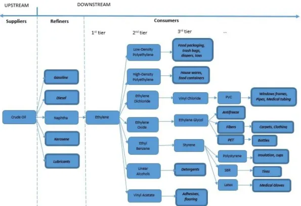
Figure 1 Petroleum Downstream Products (adapted from (Manzano, 2000) and (Profesional Logistics Group, 2013))

Crude oil and natural gas are the raw materials of the downstream petroleum industry. They are used for the production of petrochemicals and other oil derivatives. After the production of crude oil is complete from oil reserves, the crude oil undergoes a distillation process. As a result of the distillation process, various fractions of the crude oil are produced, such as fuel gas, liquefied petroleum gas, kerosene and naphtha. After cracking operations, petrochemical products such as ethylene, propylene, butadiene, benzene, toluene, and the xylenes are supplied to petrochemical plants to produce even more specialized products, such as plastics, soaps and detergents, synthetic fibers for clothes, rubbers, paints, and insulating materials. Figure 1 shows the final products that can be obtained from processing crude oil and oil derivatives.

The downstream petroleum supply chain can be characterized as a global supply-driven structure with the main following stakeholders (Manzano, 2000):

 Suppliers of crude oil: being a natural resource that is located in certain locations in the world that most of the times are far away from the main consuming countries, these stakeholders are generally members of the OECD (Organization for Economic Co-operation and Development). The main reserves of the crude oil supply are controlled by OPEC (Organization of Petroleum Exporting Countries).

 Refiners: they are located closer to final consumer all over the world because transportation of crude oil in big super-tanks is preferred versus the transportation the final product in smaller batches due to economic reasons and the strategic value that is brought for the refining assets. Hence governments often prefer to have all or part of the refinery operations in their location countries.  Consumers: are divided into small consumers and wholesale consumers. Wholesale customers

include big fuel consumers (shipping companies and airlines), power plants and petrochemical

3 4 5 6 7 8 9 10 11 12 13 14 15 16 17 18 19 20 21 22 23 24 25 26 27 28 29 30 31 32 33 34 35 36 37 38 39 40 41 42 43 44 45 46 47 48 49 50 51 52 53 54 55 56

4

facilities. Retail customers, are the ones who use fuels mainly for domestic heating and transportation.

3. Mathematical Background

Our approach uses probabilistic graphical models for the encoding of the supply chain formation problem. Probabilistic graphical models are a means for encoding probability distributions over a set of variables using graphs. In probabilistic graphical models, adjacency of nodes indicates dependence.

Furthermore, in order to encode the supply chain, we follow the concept hierarchical subtask decomposition or task dependency networks of (Walsh & Wellman, 2003). The concept of task dependency networks, does not encode dependence, hence in our encoding an arc from i to j now means i is able to supply a good which j is able to consume, rather than any notion of causality.

In order to encode preference of a producer/consumer in the supply chain we use utility functions over the contract parameters that every producer/consumer is interested in. The number of parameters of these contract may be different from producer to producer, but as long as they want to establish a commercial relationship, every pair of producer/consumer share at least one common parameters in their contracts. We will encode the utility functions for every participant in the supply chain as factors over a cluster graph.

A factor is θ is a function from Val (D) to IR. The set of variables D is called the scope the factor and denoted Scope[θ]. (Koller & Friedman 2009).

A cluster graph is a probabilistic graphical model that provides a graphical representation of the factor-manipulation process. Each node in the cluster graph is a cluster, which is associated with a subset of variables; the graph contains undirected edges that connect clusters whose scopes have some non-empty intersection (Koller & Friedman, 2009).

More formally, a cluster graph G for a set of factors θ over D is an undirected graph, each of whose nodes i is cluster associated with a subset Ci ⊆ D. A cluster graph must be family-preserving, meaning that each factor θ ϵ Θ must be associated with a cluster Ci, such that Scope[θ] ⊆ Ci. Each edge between a pair of clusters Ci and

Cj is associated with a subset Si,j⊆ Ci ∩ Cj (Koller & Friedman, 2009).

In order to incorporate risk in decision making process we use the measure of maximum expected utility (MEU). MEU provides a general framework that allows us to make decisions and associates a numerical utility to different outcomes. The utility of an agent describes his overall preferences, which can depend not only on monetary gains and losses, but also on all other relevant aspects. Each outcome o is associated with a numerical value U(o), which is a numerical encoding of the agents ”happiness” for this outcome. Importantly, utilities are not just ordinal values, denoting the agents’ preferences between the outcomes, but are actual numbers whose magnitude is meaningful. Thus, we can probabilistically aggregate utilities and compute their expectations over the different possible outcomes.

A decision-making situation D is defined by the following elements (Koller & Friedman, 2009): -a set of outcomes O = o1, ..., oN ;

-a set of possible actions that the agent can take, A = a1, ..., aK ;

-a probabilistic outcome model P: A → ΔO, which specifies a probability distribution Πa over outcomes

given that the action a was taken;

-a utility function U: O → IR, where U (o) is the agents preferences for the outcome o.

The principle of maximum expected utility asserts that, in a decision-making situation D, we should choose the action a that maximizes the expected utility: expected utility EU [D[a]] = Π

o∈O a (o) U (o).

An influence diagram represents a natural extension of the Bayesian network framework. It encodes the decision scenario via a set of variables, each of which takes on values in some space. Some of the variables are random variables, as we have seen so far, and their values are selected by nature using some probabilistic model. Others are under the control of the agent, and their value reflects a choice made by him. Finally, we also have numerically valued variables encoding the agent’s utility. This type of model can be encoded graphically, using a directed acyclic graph containing three types of nodes - corresponding to chance variables, decision variables, and utility variables. These different node types are represented as ovals, rectangles, and diamonds, respectively. An influence diagram is a directed acyclic graph over these nodes, such that the utility nodes have no children

3 4 5 6 7 8 9 10 11 12 13 14 15 16 17 18 19 20 21 22 23 24 25 26 27 28 29 30 31 32 33 34 35 36 37 38 39 40 41 42 43 44 45 46 47 48 49 50 51 52 53 54 55 56

5

More formally, in an influence diagram, the world in which the agent acts is represented by the set X of chance variables, and by a set D of decision variables. Chance variables are those decision variable whose values are chosen by nature. The decision variables are variables whose values the agent gets to choose. Each variable V∈X∪D has a finite domain Val (V) of possible values.

We can place this representation within the context of the abstract framework of definition for a decision-making situation:

-the possible actions A are all of the possible assignments Val (D); -the possible outcomes are all of the joint assignments in Val(X ∪ D).

Thus, this framework provides a factored representation of both the action and the outcome space. For a decision variable D, Pa

D is the set of variables whose values the agent knows when he chooses a value

for D. The edges incoming into a decision variable are often called information edges.

The choice that the agent makes for a decision variable D can be contingent only on the values of its parents. More precisely, in any trajectory through the decision scenario, the agent will encounter D in some particular information states, where each information state is an assignment of values to P_aD . An agent’s strategy for D must tell the agent how to act at D, at each of these information states.

A decision rule tells the agent how to act in each possible information state. Thus, the agent is choosing a local conditional model for the decision variable D. In effect, the agent has the ability to choose a conditional probability distribution for D.

More formally, a decision rule δD for a decision variable D is a conditional probability P (D|Pa_D ) - a function that maps each instantiation pa

D of PaD to a probability distribution δD over Val(D). A decision rule is

deterministic if each probability distribution δD (D|pa_D ) assigns non zero deterministic probability to exactly one value of D (Koller & Friedman, 2009).

4. Related Approaches

The first approaches for SCF (Walsh , et al., 2000), (Walsh & Wellman, 2003), (Cerquides, et al., 2003) (Collins, et al., 2002) (Cerquides, et al., 2003) addressed the problem by means of combinatorial auctions that compute the optimal SC allocation in a centralized manner. In (Walsh & Wellman, 2003) the authors proposed a mediated decentralized market protocol with bidding restrictions referred to as simultaneous ascending (M+1)st price with simple bidding (SAMP-SB), which uses a series of simultaneous ascending double auctions. SAMP-SB was shown to be capable of producing highly-valued allocations solutions which maximize the difference between the costs of participating producers and the values obtained by participating consumers over several network structures, although it frequently struggled on networks where competitive equilibrium did not exist. The authors also proposed a similar protocol, SAMP-SB-D, with the provision for de-commitment in order to remedy the inefficiencies caused by solutions in which one or more producers acquire an incomplete set of complementary input goods and are unable to produce their output good, leading to negative utility.

Recent papers that consider the SCF problem are using a message passing mechanism in graphical models in order to solve the SCF problem. In (Winsper & Chli, 2010) (Winsper & Chli, 2013), a decentralized and distributed approximate inference scheme, named Loopy Belief Propagation (LBP) was applied to the SCF problem, noting that the passing of messages is comparable to the placing of bids in standard auction-based approaches. The authors show that the SCF problem can be cast as an optimization problem that can be efficiently approximated using max-sum algorithm (Bishop, 2006). Thus, the authors offer the means of converting a SCF problem into a factor graph, on which max-sum can operate.

In LBP, the SCF problem is represented by a model in which each of the participants’ decisions is encoded in single variable. The states of each variable encode the individual decisions that the participant needs to make regarding her exchange relationships plus an inactive state. Moreover, the activation cost for a participant p is encoded by means of a simple term fp, also called activation term. Each of these activation terms has the

participant’s variable as its scope and takes value zero for the inactive state and the activation cost for any of the active states.

3 4 5 6 7 8 9 10 11 12 13 14 15 16 17 18 19 20 21 22 23 24 25 26 27 28 29 30 31 32 33 34 35 36 37 38 39 40 41 42 43 44 45 46 47 48 49 50 51 52 53 54 55 56

6

In order to ensure that decisions are consistent among participants, in LBP, there is a compatibility term for each pair of variables representing potential partners. A compatibility term fp1p2 encodes the compatibility

between the decisions of the two participants p1 and p2. Two participants are in incompatible states whenever

one of them is willing to trade with the other, but the other one does not. If two states are compatible, the value of the compatibility term is zero, otherwise is negative infinity.

As LBP suffers of scalability issues in (Penya-Alba, et al., 2012) the authors introduce the Reduced Binary Loopy Belief Propagation algorithm (RB-LBP). RB-LBP is based on the max-sum algorithm and introduces binary variables in order to encode decoupled buy and sell decisions and a selection term and an equality term to assure coherent decisions between participants. By decoupling buy and sell decisions the algorithm is able to reduce the number of combinations to take into account, making it a scalable approach even in environments with high degree of competition.

A negotiation-based task allocation method was proposed in (Kong, et al., 2015) in which every agent owns only a local view and the potential resources are found by consumers through peer-to-peer relationships. After the consumers find the potential resources, they start to negotiate with the resource providers. It is often difficult for agents to decide the optimal contract prices, so the agents have the option to negotiate with more than one potential partner, and thus the de-commitment and penalties are necessary and considered in the negotiation process.

In (Kong, et al., 2016) a decentralized approach in which providers and consumers are modelled as intelligent agents was proposed for group task allocation in dynamic environments. The proposed approach allows agents to enter and leave the environments at any time and the tasks have deadlines, and may need the collaboration of a group of self-interested providers. Each consumer has the role of an auctioneer for itself in order gather all the resources required by its task, no central authority/auctioneer being involved. The absence of a public auctioneer improves the communication and computation requirements and provides better consumer’s privacy because consumer is not required to reveal its private information to a public authority.

A pruning-decomposition loopy belief propagation-based method, called PD-LBP, was proposed in (Kong, et al., 2017) for task allocation in dynamic environments. It is composed of two phases: a pruning phase that aims at reducing the searched resource providers, and a decomposition phase that decomposes the initial network into several independent sub-networks on which is operated in parallel the belief propagation algorithm. As opposed to LBP where only the quotes of the participants are considered, the PD-LBP approach considers both a reserve price and a deadline for agreement to be accomplished.

A decentralized approach for allocating agents to tasks whose costs increase over time was proposed in (Parker, et al., 2017) aiming to minimize the increase in task. Based on max-sum algorithm (Bishop, 2006), the authors show how a distributed coordination algorithm, can be used for including costs of tasks that grow over time, enabling a wide range of problems to be solved.

5. Modelling Decision Making in Digital Supply Chains – Insights from Petroleum Industry

In the current section, we focus on digital supply chain formation and risk management providing insights from petroleum industry. We model multiple contract parameters and preferences over these parameters using utility functions. Moreover, in order to deal with risk in digital supply chains we make use of the principle of expected utility, which is the foundation for decision making under uncertainty.

The supply chain in petroleum industry presents challenges mainly due to high volatility of the prices of the raw materials and seasonal demand for the final products when compared to other commodities. In order to illustrate the decision making mechanism, we consider the position of a refinery as it is at the middle of the integrated petroleum supply chain, between the upstream and downstream. It procures crude oil from upstream assessing the price, quality, timing and distance to the refinery in order to decide the optimal acquisition. Additionally, the refiner has to carefully monitor the price risk and manage the inventory. The manufacturing activities of the refiner requires thoroughly planning and scheduling the production levels and supply chains for all the derivativesand feedstocks for petrochemical industry using tools for decision making in order to estimate market opportunities and threats under volatile market conditions.

3 4 5 6 7 8 9 10 11 12 13 14 15 16 17 18 19 20 21 22 23 24 25 26 27 28 29 30 31 32 33 34 35 36 37 38 39 40 41 42 43 44 45 46 47 48 49 50 51 52 53 54 55 56

7

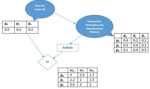
In order to model the decision mechanism for a refinery we use the influence diagram in Figure 2. The price for crude oil and predicted demand are in the form of a probability distribution and we will notate it with P(d). The price variable tells the probability that the price of the crude oil will go up, go down or stay at the same level (p0, p1, p2). The demand variables tells the probability for the evolution of the demand (d0, d1, d2) for petrochemical products when the price for the raw material will change P(d|p). We introduce, an action variable that provides a decision rule δA at action node A (Action), which is conditional probabilistic distribution P(A|Parents(A)). Parents (A) are the variables that the agent observed prior to making a decision, in the example below being the predicted demand evolution (P (A|d)).

Figure 2 Influence diagram

Hence, the action variable provides the agent with a decision situation D. Let A= {sc0,sc1,...,scm} be a set of possible actions, we want to solve the equation (1) according to the decision rule D[δA] of maximizing the

expected utility.

a∗ = argmaxa EU[D[δA]] (1)

The influence diagram in Figure 2 can be translated as a product of factors in equation (2). The first three of them are probabilistically factors and there is one numerical factor U(p,A) which represents the utility obtained by the agent depending on the evolution of the oil price and the action of choosing one of the possible supply chains (sc0,sc1,sc2).

(2) 𝐸𝑈[𝐷[𝛿𝐴]] = ∑_{𝑝,𝑑,𝐴}𝑃(𝑝)𝑃(𝑑│𝑝)𝛿𝐴(𝐴│𝑑)𝑈(𝑝,𝐴)

As we want to maximize over the decision rule δA , the equation (2) can be written as in equation (3) and if we marginalize out p, we get a factor µ(d,A). Hence, the agent has now a simple expression that is trying to optimize in equation (4), a summation over all possible values of d and A of the decision rule δ given the predicted evolution of the demand, multiplied by the factor µ(d,A) that we just computed.

(3) 𝐸𝑈[𝐷[𝛿𝐴]] = ∑_𝑑,𝐴𝛿𝐴(𝐴│𝑑)∑_𝑝𝑃(𝑝)𝑃(𝑑│𝑝)𝑈(𝑝,𝐴) (4) 𝐸𝑈[𝐷[𝛿𝐴]] = ∑_𝑑,𝐴𝛿𝐴(𝐴│𝑑)µ(𝑑,𝐴) 3 4 5 6 7 8 9 10 11 12 13 14 15 16 17 18 19 20 21 22 23 24 25 26 27 28 29 30 31 32 33 34 35 36 37 38 39 40 41 42 43 44 45 46 47 48 49 50 51 52 53 54 55 56

8

The agent will take the action A of choosing that supply chain (sc0, sc1, sc2), that will maximize the expected utility, according to his utility function and the predicted evolution of the demand d.

Having modelled the above described decision making mechanism we need to integrate it in the process of automated SCF. Hence, below we formalize the SCF problem and we describe our proposed algorithm for supply chain formation that involves the decision making mechanism described above.

Let X = {X1,X2, ..., Xn} denote set of participants in the supply chain, acted by intelligent agents. Let I = {I1,I2, ..., In} be the set of parameters that the participants in the supply chain formation process need to agree on. The participants share multiple contract parameters and SCF finishes with a contract that is composed of the actual values of the parameters that they have agreed on.

We denote by U(v) the utility that a participant gets by obtaining the actual value v =(v_I1 ,v_I2 , ..., v_Ik ) of the contract parameters. During the supply chain formation process, each agent wants to get the highest utility under the constraints from the underlying suppliers. The number of variables within the utility function may be different from one agent to other, but two agents that want to establish a commercial relationship share at least one variable in their utility functions.

We wish to find the optimal supply chain as the chain that gives to the agent representing the refinery the maximum expected utility according to his utility function while considering uncertainty conditions regarding price and demand, encoded as probability distributions.

In order to solve the problem stated above, we consider being factors, the utility functions for all the participants in the supply chain except the refinery. For the refinery we will consider as a factor the equation (4) that involves its own utility function and a probability distribution for variable price, and two conditional probability distributions for demand and for variable Action as described in the influence diagram in Figure 2. We encode the SCF problem into a graphical model - a cluster graph by considering clusters over the variables of the factors of each participant.

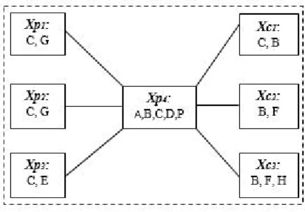
Figure 3 depicts an example of a supply chain encoded in a cluster graph, Xp4 being the refinery. Xp1, Xp2,

Xp3 represent crude oil providers for the refinery and Xc1, Xc2, Xc3 represent potential 1st tier consumers.

Figure 3 Supply chain cluster graph

In order to maintain the decentralized supply chain formation mechanism and to preserve the original graph topology we create a cluster for each agent and we assign the corresponding factor to his related cluster.

The resulted graph will be a cluster graph where the nodes are clusters Ci ⊆ {I1,I2, ..., In} and an edge between a cluster Ci and a cluster Cj is associated with a subset Si,j ⊆ Ci ∩ Cj. The subset Si,j represent the issues that the agents are talking about, the ones that they are interested in getting to an agreement, in order to form the supply chain.

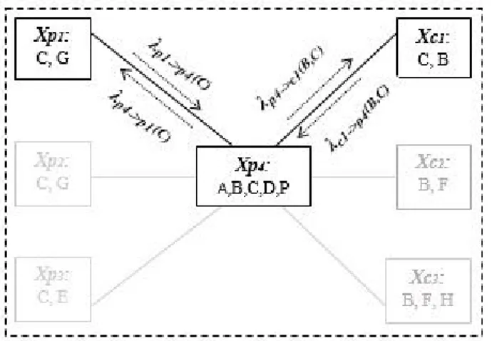
The number of variables in the utility functions might be different for two adjacent clusters and may include subjective variables that the participants don’t need to agree on. In order to eliminate variables that clusters don’t talk about we run a multiple step process in which at each step:

1. The variables that the two adjacent clusters don’t talk about are eliminated through factor maximization

3 4 5 6 7 8 9 10 11 12 13 14 15 16 17 18 19 20 21 22 23 24 25 26 27 28 29 30 31 32 33 34 35 36 37 38 39 40 41 42 43 44 45 46 47 48 49 50 51 52 53 54 55 56

9

to generate new factor λi with a smaller scope. λi is used for computing other factors.

2. A new factor τi is created through factor summation between the initial adjacent cluster and the new generated smaller factor λi.

Considering the process above in terms of message passing, the factors τi represent clusters and λi messages that are generated from cluster τi and sent to another cluster τj. These smaller factors λi that are produced by τi and consumed by τj give the messages that are passed between the two.

Among all feasible supply chains we evaluate the maximum expected utilities obtained by the refinery and find the optimal supply chain allocation as the one that maximizes it.

Figure 4 Message passing in one feasible supply chain

Figure 4 depicts an example of a feasible supply chain and the message passing process described above, between the entities in the supply chain.

In this section we described our proposed decision making mechanism and message passing algorithm for automated supply chain formation. In order to emphasize the features of our approach we used a setup for the petroleum industry, although the proposed model can be used to any complex industry with multi-level supply chains. We consider a decision-making setting with no uncertainties, for every participant in the supply chain except the refinery. Every participant has a set of possible actions and has to choose between them. Each action can lead to one of several outcomes. Most simply, the outcome of each action is known with certainty. In this case, the agents must simply select the action that leads to the outcome that is most preferred, the one that maximizes their utility function. The refinery has a decision-making situation where the outcome of an action is not fully determined because of uncertainty of price and demand evolutions. In this case, we must take into account both the probabilities of various outcomes and the preferences of the refinery between these outcomes. Hence we have modeled preferences in a complex scenario involving probability distributions for price and demand over possible outcomes.

6. Evaluation and Empirical Results

The previous approaches regarding SCF were using cost for pairwise participants in the supply chain, hence their contracts contained a single number. Our approach overcomes this limitation by proposing in section 5 a mechanism for automated SCF using multiple contract parameters that incorporates risk in decision making by making use of maximum expected utility. We need to question ourselves about the bounds for the memory needed to store preferences over the values of the parameters of the contracts. Moreover, we need to analyze the size of the messages that are sent over the clusters in our cluster graph and the overall communication requirements.

In the following we provide analysis regarding the bounds for memory requirements for storing preferences and size of the exchanged messages in the proposed decision making mechanism.

3 4 5 6 7 8 9 10 11 12 13 14 15 16 17 18 19 20 21 22 23 24 25 26 27 28 29 30 31 32 33 34 35 36 37 38 39 40 41 42 43 44 45 46 47 48 49 50 51 52 53 54 55 56

10

Memory requirements: Each agent needs to store preferences over variables’ states that are part of his utility function. Let i be the maximum number of variables in the utility function and k the maximum number of states for each parameter. Hence, the memory that an agent needs to store his preferences is θ(ki_{). Note that the memory}

requirements depend only upon the number of parameters and the number of states for each parameter. Following the literature regarding supply chain contracts in (Anupindi & Bassok, 1999) (Tsay, 1999), the average number of parameters for a contract is around eight. The preferences of each agent over the states of the variables are modelled using utility function, and their preferences are the same no matter how many agents will participate in the supply chain. Hence we can say that our approach is scalable.

Communication requirements: Two agents that are interested in establishing a commercial relationship, exchange a message regarding the variables they share in their utility functions. Let j be the maximum number of shared variables between two agents, the message size will be θ(kj_{). Let p be the number of possible allocation}

sub-graphs and let n be the maximum number of agents in each possible allocation sub-graph. The number of messages that are sent from the underling suppliers to the end consumer are (n − 1). The number of messages that are sent back from the consumer to the suppliers are also (n − 1). Hence, the communication requirements for supply chain formation mechanism is θ(p ∗ 2 ∗ (n − 1) ∗ kj).

We empirically evaluate the memory and communication requirements for the topology networks (Simple, Two consumers, Greedy Bad, Unbalanced, Many Consumers) used in previous work regarding supply chain formation (Walsh & Wellman, 2003), (Winsper & Chli, 2013), (Penya-Alba, et al., 2012).

For our experiments we used two types of data sets: 1. data sets that we called ”few parameters” that have 2-3 parameters in the utility functions with 1-2 shared parameters between them. 2. data sets that we called ”many parameters” that have 7-8 parameters in the utility functions with 5-6 shared parameters between them.

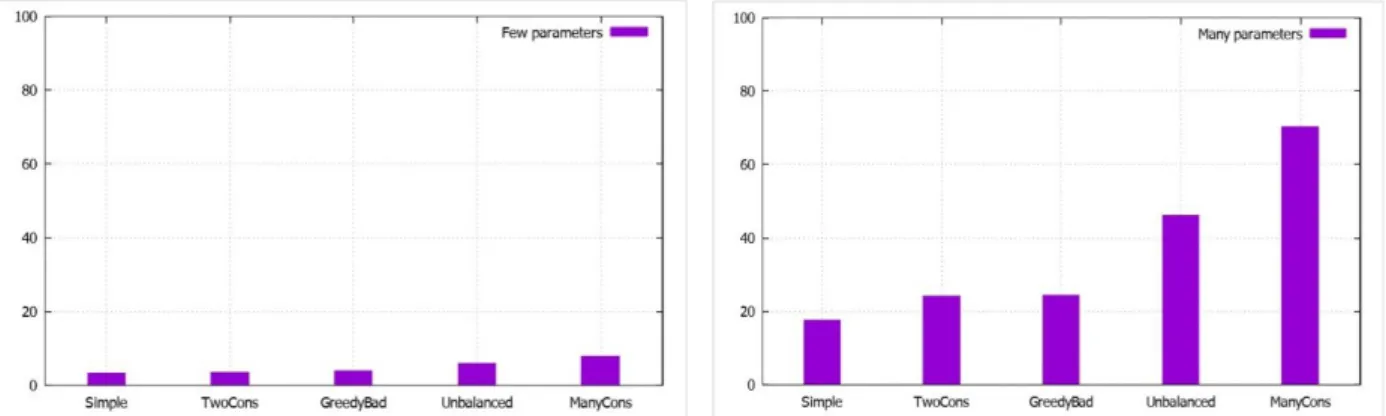
Figure 5 (a/b) Memory requirements (KB) for storing preferences - few parameters/many parameters Figure 5 depict the memory requirements for storing preferences for the two types of data sets. They show that the memory needed to store preference increases with the number of parameters in the utility functions. In real world scenarios, in most cases, the number of parameters does not exceed eight parameters, so we can conclude that is the bound memory requirement for the types of supply chain analyzed when all the parameters have two states.

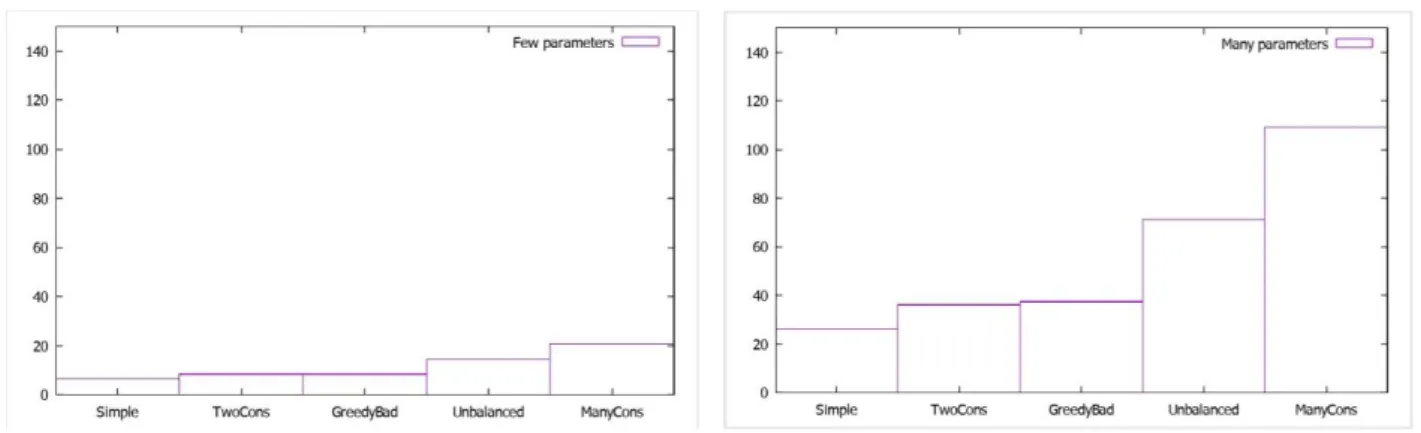
Figure 6 show that communications requirements increase according to the number of shared parameters. In the right plot the number of shared parameters is 5-6 instead of 1-2 in left plot, so the communication requirements are bigger. But, in real world scenarios as the most contract have about eight parameters maximum, means that the maximum parameters would be approximate six. We can say that the memory requirements for the types of supply chain depicted in figure 6, left plot would be the bound when the number of contract parameters of the entities involved in the supply chain are 7-8. Note that the names in the x axis in figures 5 and 6 correspond to the network structures described in (Walsh & Wellman, 2003) .

As we encode multiple contract parameters, the size of a message in our approach is bigger than the one used in previous approaches like RB-LBP because they use only binary variables. However, within the binary

3 4 5 6 7 8 9 10 11 12 13 14 15 16 17 18 19 20 21 22 23 24 25 26 27 28 29 30 31 32 33 34 35 36 37 38 39 40 41 42 43 44 45 46 47 48 49 50 51 52 53 54 55 56

11

encoding used in RB-LBP approach, the number of messages being sent at one step for two entities that want to agree upon a trading relation is six, meanwhile the number of messages that are exchanged between the entities in our approach is one, as the messages are being directly exchanged between clusters.

Figure 6 (a/b) Communication requirements (KB) -few parameters/many parameters

Our encoding has the advantage that the memory requirements for storing preferences is not dependent upon the number of concurrent suppliers in the supply chain. We use utility functions to store preference, the stored preference of an entity not being related to the number of possible suppliers/consumers in the supply chain. Hence we can conclude that our approach is scalable.

As opposed to our approach, the LPB approach stored the preferences upon trading with all other possible suppliers/consumers, hence as (Penya-Alba, et al., 2012) showed, presents scalability issues. Even though RB-LBP approach improves the performance of RB-LBP as showed in (Penya-Alba, et al., 2012) by using binary variables, it has the limitation of not dealing with complementary goods. Our approach allows for dealing also with complementary goods meanwhile still uses a scalable approach.

Hence, our approach is able to provide in a decentralized setting the following benefits over the state of the art approaches:

1. It is able to deal with multiple and flexible contract parameters making it a strong candidate for applying it in real world scenarios.

2. It extends the myopic approach for assessment of the optimal supply chain. The previous approaches evaluated the optimal supply chain based on the difference between consumption values and production costs while our approaches evaluates the optimal supply chain based on utility functions. In real world scenarios the preference over a supply chain or another depends on multiple issues that involve contract parameters that participants in the supply chain need to agree on, but also subjective parameters specific to each participant.

3. It provides the possibility to incorporate risk in the assessment of the optimal supply chain by using the measure of expected utility

4. By using utility functions in order to encode the options of the participants, we are able to incorporate multiple contract parameters meanwhile the preferences are not dependent upon the number of participants in the network. The memory requirements are dependent upon the number of contract parameters and the number of states of these parameters, hence, our approach is scalable even in markets characterized by a high degree of competition

5. The message size is dependent upon the number of shared parameters for the contract between two participants. The message size might be bigger than in other approaches like RB-LBP, because it incorporates multiple parameters, but the number of exchanged messages between two participants is lower, as a result of our encoding of the SCF problem in a cluster graph.

We must note that our approach brings several benefits over the state of the art approaches but it may have

3 4 5 6 7 8 9 10 11 12 13 14 15 16 17 18 19 20 21 22 23 24 25 26 27 28 29 30 31 32 33 34 35 36 37 38 39 40 41 42 43 44 45 46 47 48 49 50 51 52 53 54 55 56

12

a decreased performance when contract parameters take values on continuous domains. The memory needed to store the preferences of the participants and the communication requirements will grow with the size of the parameters’ domains involved in the utility functions of the participants in the supply chain.

7. Conclusion and future work

Optimizing the supply chain is critical to ensuring operational excellence and sustainability. Several approaches have been proposed in the literature regarding SCF. However we have identified important issues in the existing research literature regarding supply chain formation. First, the parameters used in order to pairwise suppliers/consumers are limited usually only at the price for traded goods. Secondly, automating supply chain formation poses an intricate coordination problem to firms that must simultaneously negotiate production relationships at multiple levels of the supply chain, but in the existing literature the resulted supply chains are assessed only using a profit optimization function for the end consumer. Thirdly, the possible risks associated with participating entities in the supply chain are not considered.

The digitization of supply chains, requires intelligent and efficient algorithms that can capture the complexity of real scenarios and can create innovative end-to-end mechanisms that connect suppliers and customers. During the supply chain formation process, in order to complete their tasks, the supply chain participants, rely upon sub-tasks that need to be completed in the production process of their input goods by producers downstream in the supply chain. In decentralized supply chain environments, as supply chain participants are primarily interested in optimizing their own objectives, optimal supply chain may require a set of actions that sometimes is not in the best interest of the participants in the supply chain. However, the optimal performance can be achieved if there can be provided a mechanism that coordinate the entities in the supply chain by contracting on a set of parameters.

Hence the current work proposed a model that uses flexible contract parameters and incorporate risk in the decision making process. We have translated the supply chain formation problem into a graphical model in which, the participants in the supply chain are represented as clusters over the variables in their utility functions, and they exchange messages regarding the variables they share in their contracts, over a cluster graph. Our approach assesses the supply chains from the perspective of an integrated supply chain bringing several benefits over previous approaches. First, the proposed approach is able to incorporate a flexible number and type of contract parameters. Secondly, as opposed to the previous approaches, our approach translates the SCF optimization problem not as a profit maximization problem but as a means for maximizing expected utility. Thirdly, the proposed decision making mechanism allows that participants in the supply chain to incorporate risk when making decisions. Moreover, the analysis and empirical evaluation provided in the sections above show that our approach has a good performance in terms of memory and communication requirements meanwhile preserving the advantages of a decentralized approach.

As noted in section above, the limitation of our approach reveals in situations where the parameters can take values over continuous domains. In these cases, storing the preferences for every agent may need a considerable amount of memory. As a future work we intend to improve performance of the proposed mechanism when we are dealing with parameters that take values over a continuous domain.

References

1. Anupindi , R. & Bassok, Y., 1999. Supply Contracts with Quantity Commitments and Stochastic

Demand. Quantitative Models for Supply Chain Management. International Series in Operations

Research & Management Science, Volume 17.

2. Bishop, C., 2006. Pattern recognition and machine learning. New York: Springer.

3. Collins, . J., Ketter, . W., Gini, M. & Mobasher, B., 2002. A multi-agent negotiation testbed for

contracting tasks with temporal and precedence constraints. International Journal of Electronic

Commerce, Volume 7.

4. Hussain, R., Assavapokee, T. & Khumawala, B., 2006. Supply Chain Management in the

Petroleum Industry: Challenges and Opportunities. International Journal of Global Logistics &

3 4 5 6 7 8 9 10 11 12 13 14 15 16 17 18 19 20 21 22 23 24 25 26 27 28 29 30 31 32 33 34 35 36 37 38 39 40 41 42 43 44 45 46 47 48 49 50 51 52 53 54 55 56

13

Supply Chain Management, 1(2), pp. 90-97.

5. J. Cerquides, U. Endriss, A. Giovannucci, J.A. Rodriguez-Aguilar, 2003. Bidding languages and

winner determination for mixed multi-unit combinatorial auctions. s.l., IJCAI, Morgan

Kaufmann Publishers Inc..

6. Koller, D. & Friedman, N., 2009. Probabilistic Graphical Models. s.l.:MIT Press.

7. Kong, Y., Zhang, M. & Ye, D., 2015. A negotiation-based method for task allocation with time

constraints in open grid environments. Concurrency and Computation: Practice & Experience,

27(3), pp. 735-761.

8. Kong, Y., Zhang, M. & Ye, D., 2016. An Auction-Based Approach for Group Task Allocation in

an Open Network Environment. The Computer Journal, 59(3), pp. 403-422.

9. Kong, . Y., Zhang, M. & Ye, D., 2017. A Belief Propagation-based Method for Task Allocation

in Open and Dynamic Cloud Environments. Knowledge-Based Systems, Volume 115, pp.

123-132.

10. M. Winsper., M. Chli, 2010. Decentralised supply chain formation: A belief propagation-based

approach. Agent-Mediated Electronic Commerce.

11. Manzano, F. S., 2000. Supply Chain Practices in the Petroleum Downstream. In: Supply Chain

Practices in the Petroleum Downstream. s.l.:Massachusetts Institute of Technology.

12. Parker, J., Farinelli, A. & Gini, M., 2017. Max-Sum for Allocation of Changing Cost Tasks.

Intelligent Autonomous System. Advances in Intelligent Systems and Computing, Volume 531,

pp. 629-642.

13. Penya-Alba, T., Vinyals, M., Cerquides, J. & Rodriguez-Aguilar, J., 2012. A scalable

Message-Passing Algorithm for Supply Chain Formation. s.l., 26th Conference on Artificial Intelligence.

14. Profesional Logistics Group, 2013. Oil&Natural Gas: The Evolving Freight Transportation

Impacts. La Quinta, CA, s.n.

15. Tsay, A., 1999. The quantity flexibility contract and supplier-customer incentives. Management

Science, Volume 45, p. 1339–1358.

16. W.E Walsh , M.P. Wellman , 2003. Decentralized supply chain formation: A market protocol

and competitive equilibrium analysis. s.l.:Journal of Artificial Intelligence Research.

17. Walsh , W. E., Wellman , M. & Ygge, F., 2000. Combinatorial auctions for supply chain

formation. s.l.:Proceedings of the 2nd ACM conference on Electronic commerce.

18. Winsper, M. & Chli, M., 2012. Using the max-sum algorithm for supply chain formation in

dynamic multi-unit environments. s.l., Proceedings of the 11th International Conference on

Autonomous Agents and Multiagent Systems.

19. Winsper, M. & Chli, M., 2013. Decentralized supply chain formation using max-sum loopy

belief propagation. Computational Intelligence, 29(2), pp. 281-309.

3 4 5 6 7 8 9 10 11 12 13 14 15 16 17 18 19 20 21 22 23 24 25 26 27 28 29 30 31 32 33 34 35 36 37 38 39 40 41 42 43 44 45 46 47 48 49 50 51 52 53 54 55 56

3 4 5 6 7 8 9 10 11 12 13 14 15 16 17 18 19 20 21 22 23 24 25 26 27 28 29 30 31 32 33 34 35 36 37 38 39 40 41 42 43 UPSTREAM Suppliers Refiners CrudeOII DOWNSTREAM 1st _tier 1 1 1 1 1 1 1 1 1 1 1 1 1 1 1 1 1 1 Ethylene 1 1 1 1 1 1 1 1 1 1 1 1 1 1 1 1 1 1 1 1 1 1 1 1 1 1 2nd_tier Low-Denslty Polyethylene HfBh-Oensity Polyethylene Ethylene Dk:hlorlde Ethylene OJdcle Ethyl Benzene Unear Alcohols Consumers 3rd _tier Foodp ...

...

ID,-,,__�

�.

,,_,,,.

.__,,_,

,.,,..._,,...

c...-�

....

,..,,,.,,.,.,

...

...,._

2 3 4 5 6 7 8 9 10 11 12 13 14 15 16 17 18 _{Po Pi P2} 19 20 0.5 0.3 0.2 21 22 23 24 25 26 27 28 29 30 31 32 33 34 35 36 37 38 39 40 41 42 43 44 45 46 47 48 49 50 51 52 53 54 SS 56 57 Action Demand for Derivatives and Petroehemieal Produets Po 3 2.5 1.7 Pi 2.2 2 1.5 P2 3.4 3 2 Po Pi P2 do di d2 0.6 0.2 0.2 0.3 0.4 0.3 0.1 0.4 0.5

3 4 5 6 7 8 9 10 11 12 13 14 15 16 17 18 19 20 21 22 23 24 25 26 27 28 29 30 31 32 33 34 35 36 37 38 39 40 41 42 43 44 45 46 47 48 49 50 51 52 53 54 SS 56 Xp1: Xc1: C,G _C,B Xp2: Xp4: Xc2: C,G _A,B,C,D,P B,F Xp3: Xc3: C,E B,F,H I'---' '---'I

---3 4 5 6 7 8 9 10 11 12 13 14 15 16 17 18 19 20 21 22 23 24 25 26 27 28 29 30 31 32 33 34 35 36 37 38 39 40 41 42 43 44 45 46 47 48 49 50 51 52 53 54 SS 56

---·

20

40

60

80

20

40

60

80

5 6 7

₁₀₀

80

60

40

20

-1

-5 6 7

₁₀₀

80

60

40

20

₀

-