Publisher’s version / Version de l'éditeur:
IEEE Transactions on Semiconductor Manufacturing, 21, 1, pp. 83-91,
2008-02-01
READ THESE TERMS AND CONDITIONS CAREFULLY BEFORE USING THIS WEBSITE. https://nrc-publications.canada.ca/eng/copyright
Vous avez des questions? Nous pouvons vous aider. Pour communiquer directement avec un auteur, consultez la première page de la revue dans laquelle son article a été publié afin de trouver ses coordonnées. Si vous n’arrivez pas à les repérer, communiquez avec nous à [email protected].
Questions? Contact the NRC Publications Archive team at
[email protected]. If you wish to email the authors directly, please see the first page of the publication for their contact information.
Archives des publications du CNRC
This publication could be one of several versions: author’s original, accepted manuscript or the publisher’s version. / La version de cette publication peut être l’une des suivantes : la version prépublication de l’auteur, la version acceptée du manuscrit ou la version de l’éditeur.
For the publisher’s version, please access the DOI link below./ Pour consulter la version de l’éditeur, utilisez le lien DOI ci-dessous.
https://doi.org/10.1109/TSM.2007.914388
Access and use of this website and the material on it are subject to the Terms and Conditions set forth at
A multi-agent based decision making system for semiconductor wafer
fabrication with hard temporal constraints
Yoon, H. J.; Shen, W.
https://publications-cnrc.canada.ca/fra/droits
L’accès à ce site Web et l’utilisation de son contenu sont assujettis aux conditions présentées dans le site LISEZ CES CONDITIONS ATTENTIVEMENT AVANT D’UTILISER CE SITE WEB.
NRC Publications Record / Notice d'Archives des publications de CNRC:
https://nrc-publications.canada.ca/eng/view/object/?id=6915e036-8b75-42ce-8fca-5260ef318492 https://publications-cnrc.canada.ca/fra/voir/objet/?id=6915e036-8b75-42ce-8fca-5260ef318492
http://irc.nrc-cnrc.gc.ca
A M u l t i - a g e n t b a s e d d e c i s i o n m a k i n g s y s t e m
f o r s e m i c o n d u c t o r w a f e r f a b r i c a t i o n w i t h h a r d
t e m p o r a l c o n s t r a i n t s
N R C C - 5 0 2 7 7
Y o o n , H . J . ; S h e n , W .
F e b r u a r y 2 0 0 8
A version of this document is published in / Une version de ce document se trouve dans: IEEE Transactions on Semiconductor Manufacturing, v. 21, no. 1, 2008, .pp 83-91
The material in this document is covered by the provisions of the Copyright Act, by Canadian laws, policies, regulations and international agreements. Such provisions serve to identify the information source and, in specific instances, to prohibit reproduction of materials without written permission. For more information visit http://laws.justice.gc.ca/en/showtdm/cs/C-42
Les renseignements dans ce document sont protégés par la Loi sur le droit d'auteur, par les lois, les politiques et les règlements du Canada et des accords internationaux. Ces dispositions permettent d'identifier la source de l'information et, dans certains cas, d'interdire la copie de documents sans permission écrite. Pour obtenir de plus amples renseignements : http://lois.justice.gc.ca/fr/showtdm/cs/C-42
A Multi-Agent Based Decision Making System
for Semiconductor Wafer Fabrication with Hard
Temporal Constraints
Hyun Joong Yoon, Member, IEEE, and Weiming Shen, Senior Member, IEEE
Abstract—This paper presents a decision making system for
semiconductor wafer fabrication facilities, or wafer fabs, with hard inter-operation temporal constraints. The decision making system is developed based on a multi-agent architecture that is composed of scheduling agents, workcell agents, machine agents, and product agents. The decision making problem is to allocate lots into each workcell to satisfy both logical and temporal constraints. A dynamic planning-based approach is adopted for the decision making mechanism so that the dynamic behaviors of the wafer fab such as aperiodic lot arrivals and reconfiguration can be taken into consideration. The scheduling agents compute quasi-optimal schedules through a bidding mechanism with the workcell agents. The proposed decision making mechanism uses a concept of temporal constraint sets to obtain a feasible schedule in polynomial steps. The computational complexity of the decision
making mechanism is proven to be O(Λ^3⋅L), where Λ is the
number of operations of a lot and L is the cardinality of the temporal constraint set.
Note to Practitioners—This paper was motivated by the
real-time scheduling problem of wafer fabs with hard temporal constraints. Existing approaches to scheduling of wafer fabs with temporal constraints generally focus on development of scheduling methods to meet due dates of orders or wafers. However, there has been little research that addresses hard temporal constraints between operations in wafer fabs. This paper proposes a novel real-time decision making method that deals with hard inter-operation temporal constraints. This paper suggests an agent-based architecture for the decision making, and presents a real-time scheduling algorithm to generate quasi-optimal schedules. The proposed scheduling algorithm consists of two procedures: FEASIBLE_SPACE and OPTIMAL_SCHED. The former finds a feasible solution space for a newly inserted lot, whereas the latter computes the optimal solution among the feasible solution space. Simulation results reveal that the proposed decision making method has sufficiently low computation time for real-time applications, and that it is effective in increasing the throughput rate of the system.
Index Terms—Semiconductor manufacturing, scheduling,
decision making systems, multi-agent systems, hard temporal constraints.
Correspondence regarding this manuscript should be addressed to Dr. W. Shen. Dr. H. J. Yoon was with National Research Council Canada, London, ON N6G 4X8, Canada. He is currently with Samsung Electronics Co. Ltd in Korea. Dr. W. Shen is with National Research Council Canada, London, ON N6G 4X8, Canada (phone: +1 (519) 430-7134; fax: +1 (519) 430-7064; e-mail: [email protected]).
I. INTRODUCTION
A wafer fabrication is a process of forming integrated circuits on wafers. An integrated circuit is composed of several layers, and requires hundreds of operations with reentrant flows. A semiconductor wafer fabrication facility, or a wafer fab, consists of workcells, each containing one or more machines. The temporal constraints have been generally considered in the context of due date based scheduling problems in wafer fabs. For instance, Lu and Kumar [11] analyzed several scheduling rules based on due dates and buffer priorities, to examine their effects on the mean delay, or equivalently manufacturing flow time, and the variance of the delay. Kim et al. [10] and Kim et
al. [9] proposed the dispatching rules that minimize mean
tardiness of orders or wafers, where the tardiness is defined as the amount of time a wafer completes past its due date. Mason
et al. [12] investigated three rescheduling strategies by
comparing their efficacies in minimizing total weighted tardiness. In addition to due dates, a temporal constraint may exist between two operations of a wafer for some technical reasons. In other words, there may exist the downstream operation that must be completed within a fixed amount of time after a specified upstream operation [23]. For instance, an operation at furnace should be started within two hours after a clean operation [19]. If a wafer violates the deadline, it must be sent back to the clean operation for reprocessing. Furthermore, the wafer that completes its furnace operation should be transferred to subsequent operation within a pre-determined time period. Otherwise, it will be needed to reheat the wafer at the furnace.
A manufacturing scheduling problem with temporal constraints can be considered as the scheduling problem of
real-time system. The real-time systems are defined as those
systems in which the correctness of the systems depends on both logical and temporal correctness [16]. The logical
correctness refers to the satisfactions of resource capacity
constraints and precedence constraints of operations. The
temporal correctness, namely timeliness, refers to the
satisfactions of the temporal constraints such as inter-operation temporal constraints and due dates. Real-time systems can be divided into those that have hard deadlines and soft deadlines. The real-time system with hard deadlines is the system in which temporal correctness is critical, whereas the one with soft
2 deadlines is the system in which temporal correctness is
important but not critical [16]. In addition, jobs of real-time systems, or wafers in wafer fabs, can be classified into three categories according to their arrival times: periodic, aperiodic, and sporadic [22]. Periodic jobs are the jobs that are activated at fixed rates, and aperiodic jobs are the jobs that are activated irregularly at arbitrary rates. Finally, sporadic jobs are the jobs that are activated irregularly, but they have minimum time bound between two consecutive activations.
The scheduling of real-time systems is to allocate resources and time to meet specified constraints and requirements. The scheduling techniques of real-time systems are mainly studied in research areas of computer science and operations research. The resources in computer science include CPU (Central Processing Unit) time and memory space, and a job typically requires only a single resource. On the other hands, the resources in operations research include machines and material handling systems, and a job typically uses subset or entire set of resources. According to Ramamritham and Stankovic [17], the scheduling techniques of real-time systems are divided into static (off-line) scheduling approaches and dynamic scheduling approaches. They state that the scheduling techniques in operations research focus more on static scheduling approaches, whereas those in computer science focus more on dynamic scheduling approaches.
Static scheduling techniques are applicable to real-time systems in which jobs are periodic. They perform off-line feasibility or schedulability analyses. For instance, static priority scheduling technique is one of the static scheduling techniques widely used in computer science community. Rate monotonic scheduling algorithm [20] is the best known static priority scheduling method, in which higher priorities are assigned to the jobs with shorter period. In operations research community, static scheduling techniques have been generally used for no-wait scheduling problems, in which jobs are not allowed to wait between two consecutive resources, and vehicle routing problems with time windows [1]. An extensive survey on the no-wait scheduling can be found in [6]. Especially, there has been a considerable amount of studies for hoist scheduling problems of no-wait manufacturing systems. Hoist scheduling techniques are generally focused on finding off-line cyclic or periodic schedules that optimize performances such as cycle time and throughput. These problems are typically solved using branch-and-bound like methods [4].
Dynamic scheduling techniques are advantageous in that system uncertainty such as aperiodic jobs and machine failures can be taken into consideration. Dynamic scheduling techniques are divided into dynamic planning-based approaches and dynamic best effort approaches [17]. In dynamic planning-based approaches, schedulability is checked at run time when a job arrives, and the job is accepted only if timeliness is guaranteed. For instance, Ramamritham et al. [18] proposed Myopic scheduling algorithm for real-time multiprocessor systems with hard deadlines. The scheduling algorithm uses the search to find a feasible schedule. On the
other hands, dynamic best effort approaches do not check schedulability at all. They try to do their best to meet temporal constraints, and therefore guarantees are not provided. Earliest deadline first (EDF) and least laxity first (LLF) are the examples of the dynamic best effort approaches [22]. Hence, dynamic planning-based approaches are adequate for the real-time systems with hard deadlines, whereas the dynamic best effort approaches are adequate for those with soft deadlines.
This paper presents a decision making system for a wafer fab with hard inter-operation temporal constraints. Dynamic
behaviors in wafer fabs such as aperiodic lot1 arrivals and
reconfiguration are taken into consideration. To achieve this goal, we adopt the dynamic planning-based approach. However, many practical scheduling problems of real-time systems in the context of both computer science and operations research are computationally intractable. Thus, this paper employs a multi-agent approach for distributed scheduling in order to meet real-time requirements, and proposes efficient scheduling algorithms to compute feasible solutions in polynomial running steps.
The rest of this paper is organized as follows: Section II describes the inter-operation temporal constraints in wafer fabs and then defines a temporal constraint workcell group; Section III proposes a multi-agent based architecture for decision making system; Section IV presents a decision making mechanism; Section V compares the proposed approach with other dispatching rules; Section VI gives concluding remarks.
II. INTER-OPERATION TEMPORAL CONSTRAINTS AND
TEMPORAL CONSTRAINT WORKCELL GROUP
Inter-operation temporal constraints are generally given in a local set of workcells, in which more than two consecutive operations are executed. We define temporal constraint
workcell group G as follows.
Definition 1: The temporal constraint workcell group G is
the set of workcells such that there is at least one inter-operation temporal constraint in G, and there is no operation flow with temporal constraints from a workcell in G to an outside workcell and vice versa.
Furthermore, minimal temporal constraint workcell group and
controllable workcell are defined as follows.
Definition 2: The temporal constraint workcell group G is minimal if and only if it includes no other temporal constraint
workcell group as a proper subset.
Definition 3: Let G be a temporal constraint workcell group.
A workcell in G is controllable if and only if it has any operation flow from an outside workcell.
1 A lot in a wafer fab implies a cassette or a FOUP (Front Opening Unified
Note that a temporal constraint workcell group G may contain more than one controllable workcell.
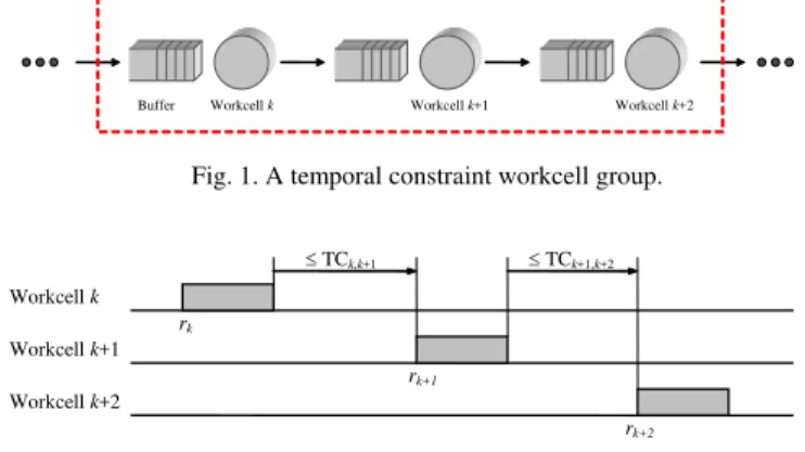
Fig. 1 illustrates a temporal constraint workcell group, in which workcell k is the controllable workcell. Inter-operation temporal constraints between workcell k and k+1, and between workcell k+1 and k+2 are denoted by TCk,k+1 and TCk+1,k+2,
respectively. The lot that completes its operation at workcell k (or workcell k+1) should start its operation at workcell k+1 (or workcell k+2) within TCk,k+1 (or TCk+1,k+2). It is sufficient to
control release times r of lots into workcell k, k+1, and k+2, in order to meet inter-operation temporal constraints, as shown in Fig. 2. Note that there is no deadline of release time for the lots in the buffer of workcell k, whereas those in the buffers of workcell k+1and k+2 have their own deadlines. It is possible for the lot in the buffer of workcell k to wait until its feasible solution is found in G. Hence, a scheduling problem in a temporal constraint workcell group is to find a release time of a lot into each workcell so that it satisfies the required temporal constraints.
Workcell k+2 Workcell k+1
Buffer Workcell k
Fig. 1. A temporal constraint workcell group.
Workcell k Workcell k+1 Workcell k+2 ≤ TCk,k+1 rk rk+1 rk+2 ≤ TCk+1,k+2
Fig. 2. Inter-operation temporal constraints.
III. ARCHITECTURE FOR DECISION MAKING
As growing the markets for non-memory semiconductors such as ASIC (Application-Specific Integrated Circuit) and SoC (System-on-Chip), the production paradigms of semiconductor industry are evolving from mass production to mass customization and from build-to-forecast to build-to-order. These new paradigms require next-generation wafer fabs to be more intelligent and agile. Centralized decision making systems with hierarchical architectures generally make decisions in a top-down manner using information transferred in a bottom-up manner. The centralized approaches may be more efficient to find optimal schedules that satisfy hard temporal constraints. However, they have some limitations for practical applications. First, they require vast quantities of real data from wafer fabs and workcells levels to machines levels. Secondly, collection of accurate data may not be practical due to the complex behaviors of machines such as cluster tools and track systems [25]. Thirdly, the practical decision making problems are too complex and large for global solutions to be formulated and implemented. Thus, the real-time decision making problems are computationally intractable. Finally,
centralized decisions become obsolete due to the stochastic and dynamic nature of wafer fabs.
Recently, there have been researches that address decision making problems in wafer fabs using agent-based approaches. For instance, Mönch et al. [15], and Mönch and Stehli [14] proposed an agent-based scheme and ontology for production control of semiconductor manufacturing processes. They presented the hierarchical multi-layer architecture based on PROSA (Product Resource Order Staff Architecture) reference architecture [24] that was developed for holonic manufacturing
systems2. The proposed architecture is composed of an entire
fab layer, a work area layer, and a work center layer. The authors used a beam-search-type algorithm to minimize the deviation of the completion time of lots from their desired due date. Yu and Huang [27] presented a model of an order fulfillment process for a foundry fab in a distributed environment using a multi-agent approach, and provided functionalities for each agent in the order fulfillment process. They classified the order fulfillment process into four categories: order management process for an interface with customers, planning process for priority setting and resource allocation, manufacturing execution process for scheduling and dispatching, and event monitoring process for data source and on-line learning. Each subprocess contains its own agent. The authors also proposed a generic message-passing platform for communication between agents and users in a distributed environment. Cheng et al. [3] proposed a systematic approach for developing holonic manufacturing execution systems for semiconductor industry. The holonic manufacturing execution system includes shop floor holon, scheduling holon, work-in-process holon, data warehouse, material handling, equipment holon, equipment, and so on. They presented seven steps for a holarchy design: constructing an abstract object model based on domain knowledge, partitioning application domain into functional holons, identifying generic parts among functional holons, developing the generic holon, defining holarchy messages, defining the holarchy framework, and designing functional holons based on the generic holon.
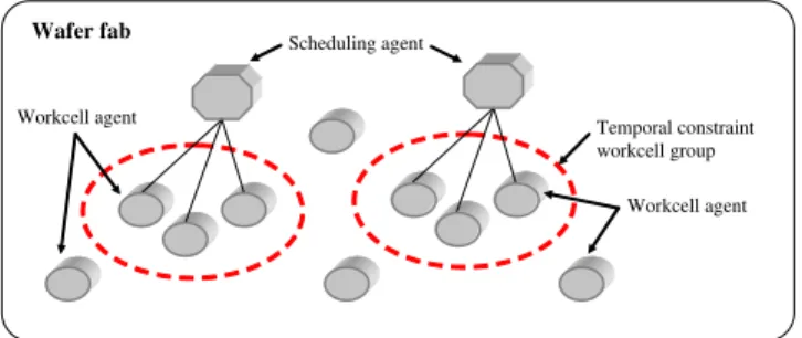
This paper presents an intelligent multi-agent based decision making system for wafer fabs. As mentioned in Section I, a multi-agent approach is applied to address the issues of complexity and flexibility. In the context of this paper, an agent is defined as a software entity with its own states, behaviors, threads of control, and an ability to interact and communicate with other entities to solve a complex problem. The proposed multi-agent based decision making system is composed of service agents, resource agents, and product agents. The service agents imply scheduling agents. The scheduling agent plays role of mediator [21]. It combines workcells with
2 Wyns [24] defines holonic manufacturing system as “a highly
decentralized manufacturing system, consisting of autonomous and co-operating agents, called holon.” Brennan and Norrie [2] discuss the difference between multi-agent system and holonic manufacturing system as follow: “unlike multi-agent systems, which is a broader software approach that can be also used for distributed intelligent control, a holonic manufacturing system is, by definition, a manufacturing-specific approach to distributed intelligent control.”
4 inter-operation temporal constraints into a temporal constraint
workcell group, and then monitors and manages them. When a lot arrives at a buffer of a controllable workcell, the scheduling agent generates a feasible schedule for the lot through cooperation with the workcell agents in the temporal constraint workcell group. The resource agents consist of workcell agents and machine agents. The workcell agents mainly play roles of dispatching lots into machines to perform their operations. The workcell agents cooperate with the scheduling agent so that the scheduling agent can compute feasible schedules, through bidding mechanism using temporal constraint sets (see Section IV for details). The machine agents perform the operations of lots assigned by a workcell agent. An operation in a machine consists of one or more sub-operations, and there may also exist temporal constraints between the sub-operations. A non-cyclic scheduling algorithm for the single-wafer processing machine with hard temporal constraints is presented in [25]. Fig. 3 shows the multi-agent based decision making architecture for a wafer fab. There are two temporal constraint workcell groups in the wafer fab, each of which is controlled by a scheduling agent. Temporal constraint workcell group Scheduling agent Workcell agent Wafer fab Workcell agent
Fig. 3. The decision making architecture in a wafer fab. The multi-agent based decision making system for a wafer fab has characteristics of distribution, autonomy, and coordination. First of all, a wafer fab is a complex system that is composed of physically distributed resources. The multi-agent approaches facilitate implementations of distributed intelligent controls in wafer fabs. The scheduling problems with inter-operation temporal constraints are decomposed into sub-problems using the concept of temporal constraint workcell group. Each thread of the scheduling agent manages one temporal constraint workcell group to guarantee both logical and temporal correctness. The scheduling agent uses only compulsory information, or temporal constraint sets, from the workcell agents to compute a feasible solution in the corresponding temporal constraint workcell group. Secondly, agents are independent and autonomous, and have their own threads of control. An agent makes decisions, depending on received stimuli, how to utilize its resources efficiently to achieve its own goal. For instance, a workcell agent continues to monitor and control their subordinates or individual machine agents. A machine in a workcell can be easily inserted and removed. Thirdly, agents communicate and cooperate with each other to achieve the goal of themselves or the entire system [7]. Temporal constraint workcell groups in a wafer fab
vary dynamically according to recipes of wafers to be fabricated and the configuration of the wafer fab. The scheduling agent creates its thread whenever a new temporal constraint workcell group is constructed, and destroys its thread whenever a temporal constraint workcell group is destructed.
IV. DECISION MAKING MECHANISM
Fig. 4 shows a sequence diagram of the decision making procedures, when a lot arrives at a buffer of a controllable workcell. The decision making mechanism consists of the following four steps.
• The scheduling agent sends information of the lot to each workcell. The information includes the low bound of the expected arrival time of the lot into each workcell, a, and operation time, TP, at each workcell.
• Each workcell computes CW that is the temporal constraint set representing available start time for the operation of the lot. The computed CW of each workcell is transferred to the scheduling agent.
• The scheduling agent finds the optimal schedule that guarantees both logical and temporal correctness, determines the release time r of the lots into each workcell, and sends it to each workcell.
• Each workcell dispatches the lots into the corresponding machine according to the schedule received from the scheduling agent. Scheduling Agent Workcell Agent a, TP Compute CW CW Dynamic planning-based scheduling r Machine Agent Dispatching lot Processing operation
Fig. 4. A sequence diagram for decision making procedures. The computed schedule does not disturb any operations of lots that are already scheduled previously. The objective of this section is to generate a feasible schedule for a minimal temporal constraint workcell group with single-route, which implies that lots have no flexible routing between workcells in the minimal temporal constraint workcell group. Batch processes of lots are not considered in this paper.
Before we describe the decision making mechanism, let us define a temporal constraint set and some operators of the temporal constraint sets. This paper uses notation of [t1, t2) to
represent time interval that follows the convention in [16]:
The temporal constraint set3 C, the set of time intervals, is defined as follows:
C = {[L1, U1), [L2, U2), ..., [Lm, Um)}. (2)
The intersection and union operators are used in the same way defined in [5].
Definition 4 [5]: Let T = {I1, I2, ..., Il} and S = {J1, J2, ..., Jm} be
two sets of constraints, i.e., sets of interval of a real variable t. (1) The intersection of T and S, denoted T ∩ S, admits only values that are allowed by both of them, namely,
T ∩ S = {K1, K2, ..., Kn}, (3)
where Kk = Ii ∩ Jj for some i and j. Note that n ≤ l + m.
(2) The union of T and S, denoted T ∪ S, admits only values that are allowed by either one of them, namely,
T ∪ S = { I1, I2, ..., Il, J1, J2, ..., Jm}. (4)
We define a new operator shifter, and two terms EARLIEST(⋅) and LATEST(⋅) as follows.
Definition 5: Let C = {[L1, U1), [L2, U2), ..., [Lm, Um)} be the set
of constraints, i.e., set of interval of a real variable t. (1) The shifter ⊕ is defined as follows:
C ⊕ [a, b) = {[L1 + a, U1 + b), [L2 + a, U2 + b), ...,
[Lm + a, Um + b)}. (5)
(2) The EARLIEST(C) is L1 and the LATEST(C) is Um.
Let us assume that a new lot arrives at a controllable workcell in a minimal temporal constraint workcell group. Oλ (λ
= 1, 2, ..., Λ) denotes λ-th operation of the lot. O1 implies the
operation at the controllable workcell, and OΛ is the last
operation in the temporal constraint workcell group. If Wλ and
aλ denote the workcell in which Oλ is to be processed and the
low bound of the arrival time of Oλ at Wλ, respectively, then aλ
is obtained as follows:
a1 = (current time), and
aλ =
∑
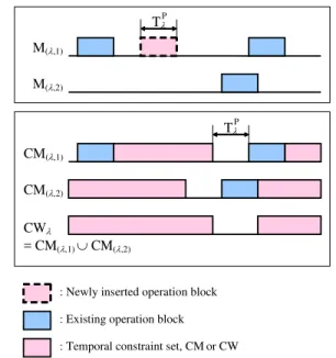
− = + 1 1 1 λ k P k T a (λ = 2, 3, ..., Λ), (6) where TkP is the operation time of Ok.At the second step, the temporal constraint set CW is computed by each workcell agent using the following procedures. Let us assume that Wλ contains a set of identical
parallel machines {M(λ,1), M(λ,2), ..., M(λ,µ(λ))}, where µ(λ) is the
number of identical parallel machines in Wλ. CM(λ,i) denotes the
temporal constraint set of M(λ,i), during one of which Oλ should
start its operation. In other words, CM(λ,i) implies a set of
available time intervals to start Oλ in M(λ,i). CM(λ,i) is computed
using following equation:
3 The temporal constraint set follows the formalism used by Dechter, Meiri,
and Pearl [5].
CM(λ,i) = {[aλ, b(λ,i))} ∩ ( CB(λ,i) ⊕ [0, −TλP) ), (7)
where CB(λ,i) is the temporal constraint set that represents the
time intervals excluding existing operation blocks in M(λ,i).
Note that the minimum time of CM(λ,i) is equal to or larger than
aλ, whereas the maximum time of CM(λ,i) is equal to or smaller
than b(λ,i). b(λ,i) is infinite in usual case. However, if machine
M(λ,i) is scheduled to be maintained or removed in near future,
b(λ,i) has a finite value. CWλ, the temporal constraint set for
available start time in Wλ, is defined as follows:
. CM )} , [ , ), , [ ), , {[ CW ) ( ~ 1 ) , ( ) ( , ) ( , , 2 , 1 , 1 ,
U
L λ μ λ λ ϕ λ λ ϕ λ λ λ λ λ λ = = = i i W W W W W W U L U L U L (8)Fig. 5 depicts the procedures to obtain CWλ.
M(λ,1) M(λ,2)
: Existing operation block : Newly inserted operation block
CM(λ,1) CM(λ,2) CWλ = CM(λ,1) ∪ CM(λ,2) TλP TλP
: Temporal constraint set, CMor CW
Fig. 5. The available start time block in Wλ with two identical parallel machines.
At the third step, the scheduling agent generates an optimal schedule using CW received from the workcell agents. The scheduling problem in the temporal constraint workcell group is the general temporal constraint satisfaction problem (TCSP) [5] that involves a set of unknown variables r1, ..., rλ , ..., rΛ,
where rλ is the release time of Oλ into Wλ. Each variable represents a time point in continuous domain. The variables have a binary constraint,
, (9) j i P i i j TR j i P i T r r T TC T + , ≤ − ≤ + ,
6 disjunctive set of unary constraint,
), ( ) ( ) ( ) ( , ) ( , 2 , 2 , 1 , 1 , W i i i W i i W i i W i W i i W i U r L U r L U r L ϕ ϕ ≤ < ∨ ∨ < ≤ ∨ < ≤ K (10)
for i = 1, 2, ..., Λ. The binary constraint (9) implies operation precedence constraint and timeliness of the newly inserted lot. and TCi,j denote transfer time and hard temporal constraint
between operation i and j, respectively. It is assumed that material handling systems are available whenever they are required to transfer lots between workcells. The disjunctive set of unary constraint (10) implies mutual exclusion requirement
in the workcell. It means that ri should be included in CWλ
shown in (8). Determining consistency for a general TCSP is proven to be NP-hard
TR j i
T
,[5]. The complexity of solving a general
TCSP is known as O(n3⋅ke), where n and e are the number of
variables, and the number of disjunctive sets of unary and binary constraints, respectively. Finally, k is the maximum number of time intervals in the disjunctive sets.
The scheduling agent solves the aforementioned TCSP to find a feasible schedule of the newly inserted lot. The proposed scheduling algorithm computes the feasible schedule that minimizes the completion time of the last operation in the temporal constraint workcell group in polynomial steps. The scheduling algorithm consists of FEASIBLE_SPACE and
OPTIMAL_SCHED procedures. The FEASIBLE_SPACE
procedure computes CSλ (λ = 1, 2, ..., Λ) for the newly inserted lot, where CSλ denotes the temporal constraint set for rλ. In
other words, CSλ represents the time intervals, during one of
which rλ should be taken place. The OPTIMAL_SCHED
procedure computes rλ (λ = 1, 2, ..., Λ) so that the completion
time of the last operation of the lot is minimized. The pseudo code of FEASIBLE_SPACE procedure is given as follows:
FEASIBLE_SPACE Input CWλ (λ = 1, 2, ..., Λ) Output CSλ (λ = 1, 2, ..., Λ) 1 λ ← 1 2 CS1 ← CW1 3 while λ < Λ 4 do λ ← λ +1 5 compute CSλ
The FEASIBLE_SPACE procedure starts by setting CS1 as
CW1. It computes CSλ from λ = 2 to λ = Λ, as increasing λ by
one. CSλ (λ = 2, 3, ..., Λ) is computed by the following equation:
λ λ λ λ {CS [ , )} CW CS 1 ~ 1 , I
I
− = + + ⊕ = k k P k TR P k k T T T CT , (11)where implies precedence
constraints and inter-operation temporal constraints with the
previous operations, and CWλ implies mutual exclusion
condition. The pseudo code of OPTIMAL_SCHED procedure is given as follows:
I
1 ~ 1 , )} , [ CS { − = + + ⊕ λ λ k k P k TR P k k T T T CT OPTIMAL_SCHED Input CSλ (λ = 1, 2, ..., Λ) Output rλ (λ = 1, 2, ..., Λ) 1 λ ← Λ 2 rλ ← EARLIEST(CSλ) 3 while λ > 1 4 do λ ← λ –1 5 rλ ← LATEST({[0, rλ+1 – TTR – TλP)}I
CSλ)The OPTIMAL_SCHED procedure computes rλ in a backward
manner to minimize the completion time of the last operation or equivalently rΛ. It starts by selecting rΛ with the earliest value in CSΛ, and then computes rλ from λ = Λ–1 to λ = 1, as decreasing
λ by one. Each rλ is selected so that its queueing time is minimized. Hence, the scheduling algorithm for the scheduling agents to compute release time r of the newly inserted lot is given as follows:
Input CWλ (λ = 1, 2, ..., Λ)
Output rλ (λ = 1, 2, ..., Λ)
1 call FEASIBLE_SPACE 2 call OPTIMAL_SCHED 3 for every λ for λ = 1, 2, ..., Λ 4 do return rλ
The computational complexity of the proposed scheduling algorithm is computed as follows. The loop on the line3-5 of
FEASIBLE_SPACE procedure is executed Λ–1 times. The
computational complexity of intersection of two temporal constraint sets having disjointed and sorted temporal constraints is known as O(l+m), where l and m are the cardinalities of two temporal constraint sets. Thus, the
complexity of the line 5 is O(Λ2⋅L), where L is the maximum
cardinality of CWλ. The total complexity of
FEASIBLE_SPACE is therefore O(Λ3⋅L). On the other hand, the
computational complexity of OPTIMAL_SCHED procedure is
O(Λ2⋅L). Accordingly, the computational complexity of the
entire scheduling algorithm is O(Λ3⋅L).
V. SIMULATION
The proposed scheduling algorithm is tested using Intel Mini Fab with five machines [8]. There are two types of lots produced and one type of test lot: Pa, Pb, and TW. All productions and test lots follow the process flow: starts >> S1 >> S2 >> S3 >> S4 >> S5 >> S6 >> outs. This paper does not consider batch process in the simulation experiments. Fig. 6 shows the layout of the workcells, and Table I shows the mapping between the processes and the machines. Transport loop goes S <> WC1 <> WC2 <> WC3 <> O. It takes 4 minutes to transfer a lot in each loop. For instance, transportation time between WC1 and WC 3 is 8 minutes.
S (Starts Warehouse) Workcell WC1 Ma Mb Me Mc Md O (Outs Warehouse) Workcell WC2 Workcell WC3
Fig. 6. Workcell layout. TABLE I
MAPPING BETWEEN PROCESSES AND MACHINES
Machine Process Description Processing Time Ma & Mb S1 & S5 Diffusion S1 = 75 mins/lot
S5 = 85 mins/lot Mc & Md S2 & S4 Ion Implantation S2 = 30 mins/lot
S4 = 50 mins/lot Me S3 & S6 Lithography S3 = 55 mins/lot
S6 = 10 mins/lot TABLE II
COMPUTING TIME
Number
of Lots Computation Time
Std. Devn. of Computation Times Average Computation Time Per Lot 10 0.0280 s 0.0052 s 0.0028 s 25 0.0675 s 0.0097 s 0.0027 s 50 0.1550 s 0.0226 s 0.0031 s 75 0.2470 s 0.0258 s 0.0033 s 100 0.3106 s 0.0244 s 0.0031 s
We define a new index deadline slackness and use four performance measures that are defined as follows:
• Deadline slackness is defined as the ratio of temporal constraint TCi,i+1 to processing time TiP, i.e., (deadline
slackness) := TCi,i+1
/
TiP.• Throughput rate is the amount of lots produced over the defined period of time.
• Cycle time is the mean elapsed time between consecutive lots completions. Cycle time is equal to the inverse of the throughput rate.
• Flow time is the time spent by a lot in a wafer fab from its entry to the exit.
• Tardiness of a lot is the sum of the whole operation
tardiness of the lot. Operation tardiness is the amount of
time that an operation is executed beyond its inter-operation temporal constraint.
It is assumed that every operation except the last operation in the Mini Fab has its own inter-operation temporal constraint. Thus, there is one temporal constraint workcell group in the Mini Fab. Table II shows the computation times in seconds of the proposed scheduling algorithm as increasing the number of lots. The computation time is obtained through 20 simulation runs for each case. Simulation is performed using a computer with Intel Mobile Pentium III 700MHz and 256MB SDRAM. The number of lots in Table II is the number of those that are currently located in the buffer of the controllable workcell.
Table II reveals that the average computation time to generate a feasible schedule for each lot is 0.0027 ~ 0.0033 seconds.
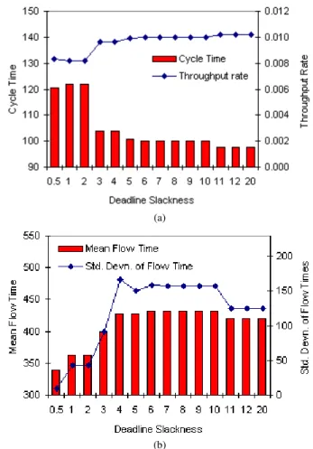
Now, we consider the case that Pa, Pb, and TW have different process flows: Pa: starts >> S1(Ma) >> S2(Mc) >> S3(Me) >> S4(Md) >> S5(Mb) >> S6(Me) >> outs, Pb: starts >> S2(Mc) >> S1(Ma) >> S3(Me) >> S5(Mb) >> S4(Md) >> S6(Me) >> outs, and TW: starts >> S4(Md) >> S5(Mb) >> S6(Me) >> S1(Ma) >> S2(Mc) >> S3(Me) >> outs. Their product ratios are assumed to be 1:1:1. Fig. 7 shows the trends of the performance measures with the deadline slackness under the proposed scheduling algorithm. Fig. 7 (a) shows that the cycle time decreases and the throughput rate increases as the deadline is getting loose. Note that the lower cycle time and the higher throughput rate are preferable. They converge to 97.74 minutes and 0.01023 wafers/minute, respectively, when the deadline slackness is over 11. The flow time is also important performance measure in wafer fabs [12]. Reductions of the mean flow time and standard deviation of flow times are encouraged to produce wafers with the higher qualities and to meet their due date. However, the reduction of the mean flow time implies decrease of the throughput rate [26]. Thus, it is needed to trade-off between them. Fig. 7 (b) reveals that the mean flow time increases with the deadline slackness. This is because the lots are allowed to spend more time in the buffers as the deadlines are getting looser. Mean flow time also converge to 420.50 minutes when the deadline slackness is over 11.
(a)
(b)
8 (a) cycle time and throughput, and (b) mean flow time and standard deviation of
flow times.
We compare the proposed scheduling algorithm with two dispatching rules: FIFO (First-In-First-Out) and EDF (Earliest Deadline First). FIFO selects the lot that arrives in the buffer at the earliest time, and EDF selects the lot with the earliest deadline. We also use WIP (Work-In-Process) rule together with the two dispatching rules in order to prevent soaring mean tardiness and mean flow time. WIP rule is to regulate the number of lots in the temporal constraint workcell group to the pre-defined WIP level. Fig. 8 shows the simulation result under EDF as increasing WIP level from 1 to 10. We set the deadline slackness to 2. This graph reveals that the cycle time decreases and then converges as the WIP level increases, which implies that the throughput rate increases and then also converges as the WIP level increases. The convergent point is related to the maximum system capacity. However, the mean flow time and the mean tardiness increase with WIP level. They diverge as the WIP level increases. As shown in Fig. 8, the mean tardiness is zero when WIP level is less than 4.
Fig. 8 Simulation results of EDF as increasing WIP level.
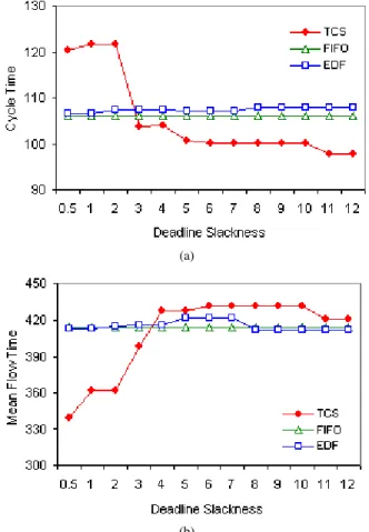
We compare the proposed scheduling algorithm with FIFO and EDF that are executed with WIP rule of WIP level 4. Fig. 9 and 10 show the simulation results that compare the proposed scheduling algorithm (TCS) and two dispatching rules. Fig. 9 shows the graph and the data table that compare the mean tardiness under the proposed scheduling algorithm, FIFO, and EDF. As shown in Fig. 9, the proposed scheduling algorithm guarantees the timeliness of the system, and EDF shows slightly better performance than FIFO in reducing the mean tardiness. FIFO results in zero mean tardiness when the deadline slackness has 9 or larger value, whereas EDF results in zero mean tardiness when the deadline slackness has 7 or larger value. Fig. 10 shows the cycle times and mean flow times under the proposed scheduling algorithm, FIFO, and EDF. As depicted in Fig. 10 (a), FIFO and EDF show the lower cycle time than the proposed scheduling algorithm with the lower deadline slackness, that is, from 0.5 to 2. However, note that FIFO and EDF have non-zero mean tardiness at that region. The proposed scheduling algorithm shows a better performance
than FIFO and EDF when the deadline slackness has 3 or larger value. Regarding the mean flow time, Fig. 10 (b) shows that FIFO and EDF are slightly outperforming the proposed scheduling algorithm in the higher deadline slackness. This is because the objective function of the proposed scheduling algorithm is to minimize the completion time of the last operation of the newly inserted lot. In other words, the proposed scheduling algorithm focuses more on decreasing cycle time, or equivalently increasing throughput rate.
Fig. 9. Comparison of mean tardiness under TCS, FIFO, and EDF.
(a)
(b)
Fig. 10. Comparison of (a) cycle time and (b) mean flow time under TCS, FIFO, and EDF.
VI. CONCLUSION
This paper proposes a decision making system for a wafer fab with hard inter-operation temporal constraints. We present a multi-agent based architecture for the decision making system, and proposes a decision making mechanism to compute a feasible schedule that satisfies both logical and temporal constraints. The best effort approaches such as dispatching rules do their best to meet system requirements. However, they have the drawbacks that they cannot guarantee timeliness which may make the system unstable due to the domino effect. Hence, this paper adopts the dynamic planning-based approach to cope with this problem. The proposed decision making method uses the bidding mechanism between agents to increase flexibility of the system and to meet real-time requirements. We introduce a new concept of the temporal constraint workcell group, and then present a bidding-based real-time scheduling algorithm with polynomial computation steps. The simulation results show that it takes sufficiently low computation time to obtain a quasi-optimal schedule using the proposed scheduling algorithm, and that the proposed scheduling algorithm is effective in increasing the throughput rate of the system.
This paper focuses on obtaining a feasible schedule in the temporal constraint workcell groups. The workcells that are not included in the temporal constraint workcell group can be controlled by various dispatching rules. For instance, the dispatching rules proposed in [9][10] help to meet due dates of the orders, and the dispatching rules proposed in [12][26] help to reduce the standard deviation of the flow times of the produced lots. Thus, the proposed decision making system can be compatible with legacy dispatching-based scheduling systems. Furthermore, the proposed decision making mechanism can take reconfiguration of the system and machine maintenance schedule into consideration, by updating the temporal constraint set CM that represents available time intervals for an operation to be executed in the corresponding machine.
REFERENCES
[1] M. O. Ball, T. L. Magnanti, C. L. Monma, and G. L. Nemhauser, Network
Routing. Amsterdam: Elsevier Science B. V., 1995.
[2] R. W. Brennan and D. H. Norrie, “Agents, holons and function blocks: Distributed intelligent control in manufacturing,” Journal of Applied
Systems Studies, vol. 2, no. 1, pp. 1-19, 2001.
[3] F. T. Cheng, C. F. Chang, and S. L. Wu, “Development of holonic manufacturing execution systems,” Journal of Intelligent Manufacturing, vol. 15, pp. 253-267, 2004.
[4] H. Chen, C. Chu, and J. M. Proth, “Cyclic scheduling of a hoist with time window constraints,” IEEE Transactions on Robotics and Automation, vol. 14, no. 1, pp. 144-152, 1998.
[5] R. Dechter, I. Meiri, and J. Pearl, “Temporal constraint network,”
Artificial Intelligence, vol. 49, pp. 61-95, 1991.
[6] N. G. Hall and C. Sriskandarajah, “A survey of machine scheduling problems with blocking and no-wait in process,” Operations Research, vol. 44, no. 3, pp. 510-525, 1996.
[7] M. N. Huhns and L. M. Stephens, “Multiagent systems and societies of agents,” in Multiagent Systems: A modern approach to distributed
artificial intelligence, G. Weiss, Cambridge, MA: MIT Press, 1999, pp.
79-120.
[8] K. Kempf. Intel five-machine six step mini-fab description. Intel/ASU
Report [online].
http://www.eas.asu.edu/~aar/research/intel/papers/fabspec.html.
[9] Y. D. Kim, J. G. Kim, B. Choi, and H. U. Kim, “Production scheduling in a semiconductor wafer fabrication facility producing multiple product types with distinct due dates,” IEEE Transactions on Robotics and
Automation, vol. 17, no. 5, pp. 589-598, 2001.
[10] Y. D. Kim, J. U. Kim, S. K. Lim, and H. B. Jun, “Due-date based scheduling and control policies in a multiproduct semiconductor wafer fabrication facility,” IEEE Transactions on Semiconductor
Manufacturing, vol. 11, no. 1, pp. 155-154, 1998.
[11] S. H. Lu and P. R. Kumar, “Distributed scheduling based on due dates and buffer priorities,” IEEE Transactions on Automatic Control, vol. 36, no. 12, pp. 1406-1416, 1991.
[12] S. H. Lu and D. Ramaswamy, and P. R. Kumar, “Efficient scheduling policies to reduce mean and variance of cycle-time in semiconductor manufacturing plants,” IEEE Transactions on Semiconductor
Manufacturing, vol. 7, no. 3, pp. 374-388, 1994.
[13] S. J. Mason, S. Jin, and C. M. Wessels, “Rescheduling strategies for minimizing total weighted tardiness in complex job shop,” International
Journal of Production Research, vol. 42, no. 3, pp. 613-628, 2004.
[14] L. Mönch and M. Stehli, “An ontology for production control of semiconductor manufacturing processes,” in Proceedings of the First
German Conference on Multiagent System Technologies, Erfurt,
Germany, September 22-25, 2003.
[15] L. Mönch, M. Stehli, and J. Zimmerman, “FABMAS: An agent-based system for production control of semiconductor manufacturing processes,” in Proceedings of the First International Conference on
Industrial Application of Holonic and Multi-Agent Systems, Prague,
Czech Republic, September 1-3, 2003.
[16] N. Nissanke, Realtime system. London: Prentice Hall, 1997. [17] K. Ramamritham and J. A. Stankovic, “Scheduling algorithm and
operating systems support for real-time systems,” Proceedings of the
IEEE, vol. 82, no. 1, pp. 55-67, 1994.
[18] K. Ramamritham, J. A. Stankovic, and P. F. Shiah, “Efficient scheduling algorithms for real-time multiprocessor systems,” IEEE Transactions on
Parallel and Distributed Systems, vol. 1, no. 2, pp. 184-194, 1990.
[19] J. K. Robinson, “Capacity planning in a semiconductor wafer fabrication facility with time constraints between process steps,” Ph. D. Dissertation, Department of Mechanical and Industrial Engineering, University of Massachusetts, Amherst, 1998.
[20] L. Sha, R. Rajkumar, and S. S. Sathaye, “Generalized rate-monotonic scheduling theory: A framework for developing real-time systems,”
Proceedings of the IEEE, vol. 82, no. 1, pp. 68-82, 1994.
[21] W. Shen, “Distributed manufacturing scheduling using intelligent agents,” IEEE Intelligent Systems, vol. 17, no. 1, pp. 88-94, 2002. [22] J. A. Stankovic, M. Spuri, K. Ramamritham, and G. C. Buttazo, Deadline
scheduling for real-time systems: EDF and related algorithms. Norwell,
MA: Kluwer Academic Publishers, 1998.
[23] H. Watts, “Improving fab performance,” Future Fab International, vol. 9, July 2000.
[24] J. Wyns, “Reference architecture for holonic manufacturing systems: The key to support evolution and reconfiguration,” Ph. D. Dissertation, Department of Mechanical Engineering, Katholieke Universiteit Leuven, Belgium, 1999.
[25] H. J. Yoon, “Real-time scheduling of semiconductor integrated single-wafer processing tools,” Ph. D. Dissertation, Department of Mechanical Engineering, Korea Advanced Institute of Science and Technology, Daejeon, Republic of Korea, 2004.
[26] H. J. Yoon and D. Y. Lee, “A control method to reduce the standard deviation of flow time in wafer fabrication,” IEEE transactions on
Semiconductor Manufacturing, vol. 13, no. 3, pp. 389-392, 2000.
[27] C. Y. Yu and H. P. Huang, “Development of the order fulfillment process in the foundry fab by applying distributed multi-agents on a generic message-passing platform,” IEEE/ASME Transactions on Mechatronics, vol. 6, no. 4, pp. 387-398, 2001.