What does reflection from cloud sides tell us about vertical distribution of cloud droplet sizes?

(1)

HAL Id: hal-00302035

https://hal.archives-ouvertes.fr/hal-00302035

Submitted on 31 Jul 2006

HAL is a multi-disciplinary open access

archive for the deposit and dissemination of sci-entific research documents, whether they are pub-lished or not. The documents may come from teaching and research institutions in France or abroad, or from public or private research centers.

L’archive ouverte pluridisciplinaire HAL, est destinée au dépôt et à la diffusion de documents scientifiques de niveau recherche, publiés ou non, émanant des établissements d’enseignement et de recherche français ou étrangers, des laboratoires publics ou privés.

What does reflection from cloud sides tell us about

vertical distribution of cloud droplet sizes?

A. Marshak, J. V. Martins, V. Zubko, Y. J. Kaufman

To cite this version:

A. Marshak, J. V. Martins, V. Zubko, Y. J. Kaufman. What does reflection from cloud sides tell us about vertical distribution of cloud droplet sizes?. Atmospheric Chemistry and Physics Discussions, European Geosciences Union, 2006, 6 (4), pp.7207-7233. �hal-00302035�

(2)

ACPD

6, 7207–7233, 2006

Vertical distribution of cloud droplet sizes

A. Marshak et al. Title Page Abstract Introduction Conclusions References Tables Figures J I J I Back Close Full Screen / Esc

Printer-friendly Version Interactive Discussion

EGU

Atmos. Chem. Phys. Discuss., 6, 7207–7233, 2006 www.atmos-chem-phys-discuss.net/6/7207/2006/ © Author(s) 2006. This work is licensed

under a Creative Commons License.

Atmospheric Chemistry and Physics Discussions

What does reflection from cloud sides tell

us about vertical distribution of cloud

droplet sizes?

A. Marshak1, J. V. Martins1,2, V. Zubko3, and Y. J. Kaufman3

1

NASA – Goddard Space Flight Center, Climate and Radiation Branch, Greenbelt, MD, USA 2

Joint Center for Earth Systems Technology, University of Maryland Baltimore County, Baltimore, MD, USA

3

Nortel Government Solutions, Inc., Lanham, MD, USA

Received: 2 May 2006 – Accepted: 1 June 2006 – Published: 31 July 2006 Correspondence to: A. Marshak ([email protected])

(3)

ACPD

6, 7207–7233, 2006

EGU Abstract

Cloud development, the onset of precipitation and the effect of aerosol on clouds de-pend on the structure of the cloud profiles of droplet size and phase. Aircraft measure-ments of cloud profiles are limited in their temporal and spatial extent. Satellites were used to observe cloud tops not cloud profiles with vertical profiles of precipitation-sized

5

droplets anticipated from CloudSat. The recently proposed CLAIM-3D satellite mission (cloud aerosol interaction mission in 3-D) suggests to measure profiles of cloud micro-physical properties by retrieving them from the solar and infrared radiation reflected or emitted from cloud sides.

Inversion of measurements from the cloud sides requires rigorous understanding of

10

the 3-dimentional (3-D) properties of clouds. Here we discuss the reflected sunlight from the cloud sides and top at two wavelengths: one nonabsorbing to solar radia-tion (0.67 µm) and one with liquid water efficient absorption of solar radiation (2.1 µm). In contrast to the plane-parallel approximation, a conventional approach to all current operational retrievals, 3-D radiative transfer is used for interpreting the observed

re-15

flectances. General properties of the radiation reflected from the sides of an isolated cloud are discussed. As a proof of concept, the paper shows a few examples of radia-tion reflected from cloud fields generated by a simple stochastic cloud model with the prescribed vertically resolved microphysics. To retrieve the information about droplet sizes, we propose to use the probability density function of the droplet size distribution

20

and its first two moments instead of the assumption about fixed values of the droplet effective radius. The retrieval algorithm is based on the Bayesian theorem that com-bines prior information about cloud structure and microphysics with radiative transfer calculations.

(4)

ACPD

6, 7207–7233, 2006

EGU 1 Introduction

Investigation of cloud development and the onset of precipitation are essential to under-stand the role of clouds in the hydrological cycle and the effect of pollutants on clouds and precipitation (Ramanathan et al., 2001). It also advances our understanding of the feedback of clouds on climate change and the aerosol indirect forcing of climate

5

through cloud modification. Therefore, we have to resolve the vertical distribution of cloud droplet sizes and determine the temperature of glaciation for clean and polluted clouds (Andreae et al., 2004). Knowledge of the droplet vertical profile is also essential for understanding precipitation (Rosenfeld, 2000; Rosenfeld and Ulbrich, 2000). In an accompanied paper, Martins et al. (2006)1 suggest a satellite mission to derive

pro-10

files of the cloud microphysics using observations of the cloud sides. Here we show a methodology, based on 3-dimensional (3-D) cloud properties to retrieve the cloud profiles from the new satellite measurements.

So far, all existing satellites either measure cloud microphysics only at cloud top (e.g., Moderate Resolution Imaging Spectrometer (MODIS), see Platnick et al., 2003)

15

or give a vertical profile of precipitation sized droplets (e.g., CloudSat, see Stephens et al., 2002). Note that the combination of millimeter-wave radar reflectivity measured by CloudSat with MODIS (on Aqua) measurements of solar radiance will be able to provide cloud droplet size vertical profiles but under some strong assumptions of given number concentration and droplet size distribution.

20

Except for Polarization and Directionality of the Earth’s Reflectance (POLDER) that retrieves cloud droplet effective radius at the very top cloud layer (with an optical thick-ness of 1) from polarization measurements of the reflected light (e.g., Breon and Golub, 1998; Breon and Doutriaux-Boucher, 2005), all operational retrievals of cloud droplet size are based on spectral observations (e.g., Nakajima and King, 1990). For MODIS,

25

1

Martins, J. V., Kaufman, Y., Marshak, A., Rosenfeld, D., Remer, L., and Koren, I., Fernandez-Borda, R.: Remote sensing of the aerosol effect on the vertical profile of cloud microphysics and thermodynamics, Atmos. Chem. Phys. Discuss., in preparation, 2006.

(5)

ACPD

6, 7207–7233, 2006

EGU

cloud optical thickness, τ, and droplet effective radius, r_e, are simultaneously derived from various two band combinations: typically one water-absorbing band {1.6, 2.1, or 3.7 µm} and one nonabsorbing band {0.65, 0.86, or 1.2 µm} (Platnick et al., 2003). Since water absorbs differently in the three MODIS absorbing bands, the less absorb-ing 1.6-µm band and the more absorbabsorb-ing 3.7-µm band complement to the 2.1-µm band

5

for assessing the vertical variation of r_ein the upper portion of the cloud (Platnick, 2000; Chang and Li, 2002). However, these variations are not sufficient to resolve the vertical distribution of cloud droplet sizes from cloud base to cloud top. What is if one would measure the vertical profiles of the cloud microphysical properties by retrieving them from the solar (and infrared) radiation reflected (or emitted) directly from cloud sides?

10

Note that all existing operational retrieval algorithms are based on the plane-parallel approximation that does not take into account the cloud horizontal inhomogeneity. In terms of cloud aspect ratio, A=L/h (where L and h are horizontal and vertical dimen-sions of a cloud, respectively), the main plane-parallel assumption used for any remote sensing retrieval is that A is infinitely large and that the satellite always sees the cloud

15

top. Hence, a pair of reflectances at the nonabsorbing and absorbing bands indicates how optically thick (thus estimates τ) and how absorbing (thus estimates r_e) clouds are (Nakajima and King, 1990).

It is well understood that finite isolated clouds of various shapes and sizes can have absolutely different radiative properties than their plane-parallel counterparts. Davies

20

(1978) represented an isolated cloud as a cuboid of given dimensions. In this case, the incident solar beam hits not only the top of the cloud but also one or two of its sides. As an alternative to the plane-parallel model to simulate cumulus clouds, recently Davis (2002) used a spherical turbid medium. For his spherical cloud, he was able to derive analytically the transmitted and reflected fluxes in terms of the cloud optical diameter.

25

He showed that these results could be used to estimate the cloud optical diameter from radiances reflected from dark and bright sides of clouds.

In general, if one releases the assumption that the aspect ratio A is infinitely large then, in addition to cloud tops, a satellite-based observer will likely see cloud sides.

(6)

ACPD

6, 7207–7233, 2006

EGU

Because of a variety of possible aspect ratios and cloud geometrical shapes, the situ-ation seems to be out of control and measured data cannot be correctly interpreted in the sense of cloud properties. Similar to the plane-parallel approximation, in order to bring the retrieval back under control we have to make simplifying assumptions. The main assumption for cloud side remote sensing is that regardless of the aspect ratio,

5

cloud geometrical shape and its microphysical structure, a pair of reflectances at non-absorbing and non-absorbing bands determines a distribution of droplet sizes. Note that this is an assumption rather than a statement since it can’t be checked with the model calculation and inversion for all cloud types. Also note that here we are talking about the distribution of droplet sizes (with mean and standard deviation) rather than a single

10

value. Finally, together with the brightness temperature this assumption allows us to estimate a vertical profile of droplet (particle) sizes (Martins et al., 20061).

Of course, the above assumption will not work for all cloud types like the plane-parallel approximation does not work for all clouds either. Here we will consider only optically thick clouds (τ≥40) with relatively small aspect ratio (L/h≤2–5). We will

fur-15

ther make some additional limitations regarding the satellite viewing angles. In order to see a sufficient amount of cloud sides, the viewing zenith angles, θ, will be limited to more oblique angles of θ≥45◦. For simplicity here we will be considering only “back-ward” directions, i.e., ϕ≈ϕ₀where ϕ₀and ϕ are solar and viewing azimuthal angles, respectively. Under these rather strong limitations, the paper proves the concept of a

20

possible retrieval of the distributions of droplet vertical profiles using three bands: non-absorbing, water absorbing and brightness temperature. The latter is associated with the measured height and is discussed in the companion paper (Martins et al., 2006)1.

The plan of the paper is as follows. Section 2 briefly discusses the main radiative transfer features of the reflectance from cloud sides based on a single homogeneous

25

cloud. To generalize these results to a more realistic horizontally inhomogeneous cloud field, Sect. 3 describes simple stochastic and microphysical models used to simulate a variety of cloud fields. With the help of two wavelengths at 0.67 and 2.1 µm, Sect. 4 demonstrates the retrievals of the distribution of droplet sizes from the measurements

(7)

ACPD

6, 7207–7233, 2006

EGU

of radiation reflected from the cloud fields simulated in Sect. 3. At the end of Sect. 4, this approach is generalized in the terms of Bayesian retrievals (McFarlane et al., 2002; Evans et al., 2002). Finally Sect. 5 provides general discussion and summarizes the results.

2 Radiative transfer calculations

5

2.1 3-D radiative transfer tools

There are two 3-D Radiative Transfer (RT) tools that dominate atmospheric radiation applications and are currently the only available options for solving complex RT prob-lems: the Spherical Harmonic Discrete Ordinate Method (SHDOM) of Evans (1998) and the Monte Carlo (MC) method (Marchuk et al., 1980). When many radiative

quan-10

tities are required, e.g., the radiance field across cloud top, SHDOM is much faster than MC, but its errors (and limitations) are harder to interpreter, especially for opti-cally thick and highly variable media around cloud edges. Since the rule-of-thumb in using SHDOM requires the optical path across a grid cell to be of order of one, its solu-tion may be not accurate for horizontally and vertically thick clouds. Moreover, SHDOM

15

(tri)linearly interpolates the extinction between grid points; thus it may have some prob-lems when reflectance from cloud sides of optically thick clouds is calculated. Anyway, in this study we used both MC and SHDOM; for several key calculations both meth-ods were applied simultaneously to the same set of cloud parameters to intercompare and validate the results. To the best of our knowledge, the results shown in the paper

20

are numerically accurate. (For the detailed description of both the SHDOM and MC methods, see Evans and Marshak, 2005).

2.2 Main radiative transfer features of the reflectance from cloud sides

Using a 3-D Monte Carlo radiative transfer code (Evans and Marshak, 2005), we calculated reflectance at 0.67 and 2.1 µm wavelengths from a single homogeneous

(8)

ACPD

6, 7207–7233, 2006

EGU

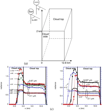
cloud. The cloud top was simulated by an infinitely long rectangular shape with width

L=12.8 km and height h=2 km (Fig. 1a). Cloud vertical optical thickness, τ, varied

from 20 to 160 and droplet effective radius was assumed a constant r_e=10 µm. The cloud was illuminated at solar zenith angle (SZA) θ₀=60◦ along cloud inhomogeneity and observed at viewing zenith angles (VZA) θ=45◦–70◦ from the illuminated side of

5

the cloud. The reflectances are plotted in panels (b) and (c) on Fig. 1. The horizontal axis shows the distance to the cloud edge (negative x-values) and the distance from the cloud edge (positive x-values). The cloud edge is located at x=0. For example, a cloud side, viewed at θ=70◦, can be seen h×tan(θ)=5.5 km away from the cloud (neg-ative 5.5 km). Thus neg(neg-ative x-values correspond to radiation reflected from a cloud

10

side while positive x-values to radiation reflected from a cloud top. Here are the main features that can be observed from these two panels.

– Reflectance from a cloud side at 2.1 µm is saturated starting from τ=40 while

reflectance at 0.67 µm does not reach the level of saturation at all or will be saturated only at very large values of cloud optical thickness τ. The maximum

15

2.1 µm reflectance from cloud sides, I_side(θ₀,θ), depends on both SZA, θ₀, and VZA,θ. It can be estimated as

I_side(θ₀, θ) ≤ I_pp(90◦− θ₀, 90◦− θ, ϕ − ϕ₀_{= 180}◦, τ=∝) cos(90◦− θ₀)/ cos(θ₀), (1a)

where I_pp(θ₀, θ, ϕ–ϕ₀, τ) is the cloud top reflectance calculated using the plane-parallel approximation (Stamnes et al., 1988). For example, for θ₀=θ=60◦, the 2.1 µm

20

reflectance

I_side(60◦, 60◦) ≤ I_pp(30◦, 30◦, ϕ− ϕ₀= 180◦, τ = 160) cos(30◦)/ cos(60◦)= 0.782, (1b) as seen in panel b.

– The more oblique viewing zenith angle θ (or the larger cloud side, h) the wider

the area of maximal reflectance at 2.1 µm (panel c).

(9)

ACPD

6, 7207–7233, 2006

EGU – For optically and geometrically thick clouds, the reflectance from cloud side near

cloud top is smaller than the one reflected from the middle of the cloud side. This effect is much more pronounced for 0.67 µm than for 2.1 µm.

– For thick clouds, starting from a few optical depths away from cloud edges,

re-flectance from cloud top at 2.1 µm is well approximated by the plane-parallel

ap-5

proximation. Depending on the extinction coefficient, it is not always the case for reflectance at 0.67 µm. At both wavelengths reflectance from cloud top increases towards the illuminated side and decreases towards the shadowed side.

– Finally, the number of measurements from cloud side is equal to h×tan(θ)/s where

s is the horizontal resolution of a radiometer. For example, if h=2 km, θ=70◦, and

10

s=0.1 km, there will be 55 cloud side measurements.

All of the above radiative transfer features will be observed by analyzing the reflectance from more complex cloud fields.

2.3 Reflectance from cloud sides for a cloud with variable droplet sizes

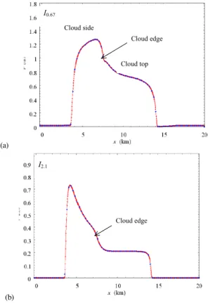
Figure 2 shows an example of reflectances from cloud side and cloud top for the same

15

two wavelengths (0.67 µm and 2.1 µm) but with droplet effective radius r_e increasing linearly with height from 5 µm (at the cloud base) to 25 µm (at the cloud top). Cloud geometrical thickness h=4 km and cloud optical thickness is τ=80 (thus extinction co-efficient is 20 km−1). With horizontal resolution s=0.25 km and VZA θ=45, there are

h×tan(θ)/s=16 cloud side “measurements.” As for a simple example in Fig. 1, I_0.67 20

reaches its maximum near cloud top (actually about 1 km from the cloud top) where yet most of the photons are reflected back from the cloud side without either transmitting through cloud and escaping from cloud base or reflecting from cloud top. Unlike in the previous example, the horizontal size L of a cloud is only 6.5 km and with the ex-tinction coefficient 20 km−1 this is not sufficient to reach a stable plane-parallel regime

25

(10)

ACPD

6, 7207–7233, 2006

EGU

the shadowed one. In contrast, I_2.10 has a flat plateau of 5 km across where the 3-D reflectance perfectly matches the plane-parallel one. Because of increasing droplet sizes with height, the maximum is reached much lower than in case of conservative scattering. It is around 1 km from cloud base where r_e=9–11 µm. With farther increase of r_e, reflectance I_2.10 drops fast and reaches a flat plane-parallel level already at the

5

cloud top (r_e=25 µm) about 1 km from the cloud edge.

The study of reflectance from an isolated finite-size cloud is not new and has begun yet in early 70-ies (see, e.g., McKee and Cox, 1974; Davies 1978 and 1984). As it is seen from Figs. 1 and 2, cloud side reflectances at the two (water-absorbing and nonabsorbing) wavelengths, have well-determined features. Not unlike their cloud top

10

counterparts in the plane-parallel approximation (Nakajima and King, 1990), the com-bination of these two reflectances can be mapped into retrievals of cloud optical (τ) and microphysical (r_e) structure. The key question here is whether these features survive if applied to realistic cloud fields rather than a single isolated horizontally homogeneous cloud. Next we briefly discuss cloud models used in this study.

15

3 Cloud models

Realistic 3-D cloud fields, as an input in radiative transfer calculations, can be ob-tained from either dynamical or stochastic cloud models. For the purpose of this paper (to learn what reflection from cloud sides tells us about vertical distribution of cloud particles), a choice of model is not very crucial. The main requirements for a model

20

were set as to have a field of several joined and disjoined clouds with the prescribed (observed) mean, standard deviation and correlation function of variable cloud optical thickness τ(x, y) with a desired cloud fraction A_c and cloud top height h(x, y). Hav-ing some experience in stochastic cloud modelHav-ing (e.g., Marshak et al., 1994; Prigarin and Marshak, 2005), we selected a broken cloud version (Marshak et al., 1998) of a

25

simple fractionally integrated cascade model (Schertzer and Lovejoy, 1987) that gener-ates cloud fields with a given power spectral exponent, mean and standard deviation of

(11)

ACPD

6, 7207–7233, 2006

EGU

cloud optical thickness. To correlate τ(x, y) with h(x, y), we generated independently a τ(x, y)-field and the mean photon free path field l (x, y). The cloud geometrical thick-ness field (assuming cloud base to be a constant) is thus a product between the optical depth and the mean free path fields,

h(x, y)= τ(x, y) × l(x, y) (2)

5

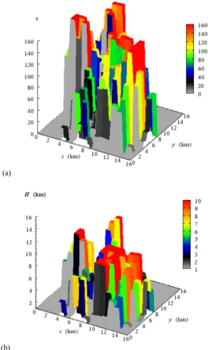
Figure 3 illustrates one realization of a cloud with an array of optical and geometrical thicknesses. Though it might not look very realistic, it preserves the observed correla-tion funccorrela-tion in both optical and geometrical thicknesses.

After cloud structure, cloud microphysics is perhaps the most important cloud model feature needed for radiative transfer calculations. For simplicity and for more

straight-10

forward interpretation of the simulated radiative transfer results, we made two assump-tions:

– cloud droplets grow linearly with z, i.e.,

r_e(z; x, y)= a(z − z₀)+ b, z₀≤ z ≤ h(x, y),a and b are constants (3a)

– the extinction coefficient σ_extdoes not depend on z, i.e.,

15

σext(z; x, y) ≡ σext(x, y). (3b)

Note that under some general assumptions (e.g., Platnick, 2000), cloud liquid water content (LWC) is proportional to a product of the density of liquid water, ρ, cube of the droplet effective radius, r_e, and the total number of droplets in unit volume, N,

LW C(z; x, y) ≈4

3πρr

3_{(z; x, y)N(z; x, y).} _(4a)

20

Cloud LWC is also related to τ, r_e, and ρ as (Stephens, 1994, p. 219)

τ(x, y)= 3 2ρ h(x,y) Z 0 LW C(z; x, y) r_e(z; x, y) d z. (4b)

(12)

ACPD

6, 7207–7233, 2006

EGU

Therefore, with the assumptions (3a–b), N changes with vertical coordinate z as r_e−2, namely, N(z; x, y)= τ(x, y) 2πh(x, y) 1 r_e2(z; x, y) = 1 2π σext(x, y) r_e2(z; x, y) . (5a)

At the cloud base for z= z₀, we get

N(z₀; x, y)= 1 2π

σext(x, y)

b2 . (5b)

5

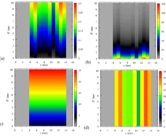
For example, for r_e(z₀)= b=5 µm and σ_ext=20 km−1one gets N(z₀)=127 cm−3. If at the cloud top r_e=25 µm then Eq. (5a) yields N(z₀)=5 cm−3. Figure 4 shows an example of vertical profiles for cloud liquid water, LWC (in g/m3), total number of drops, N(in cm−3), effective radius, r_e (in µm), and extinction coefficient, σ_ext(in km−1). We see that, for each x and y, with z increasing from cloud base z₀ to cloud top h(x,y), LWC and r_e

10

increase linearly, N decreases as z2, and σ_extis constant.

4 Proof of concept

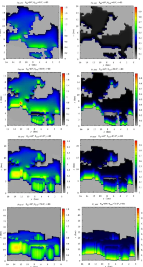
Figure 5 shows an example of reflectances from a 16 by 16 km cloud field illuminated at θ₀=60◦ [from South (bottom of the image)] and viewed at different viewing angles:

θ=0◦, 20◦, 45◦, and 70◦ (also from South). The cloud is 4 km thick; for illustrative

15

purposes, the cloud top is flat. Droplet effective radius grows linearly with height from 5 to 25 µm; thus in Eq. (3a), a=5 and b=5 µm.

The two upper plots show nadir angle observations. As illustrated in Figs. 1 and 2, we see that at 0.67 µm, the cloud tops at the illuminated cloud edges are much brighter, whereas the cloud tops at the opposite ends look darker than in the rest of

20

the area. At 2.1 µm, cloud tops are homogeneous except may be the first 0.5 km away from the illuminated cloud edges. With increasing viewing angles, we start seeing

(13)

ACPD

6, 7207–7233, 2006

EGU

illuminated cloud sides that are brighter than their cloud top counterparts. As a result, even visually one can distinguish between cloud sides and cloud tops, especially at low viewing angles. Similar to Fig. 2, at 0.67 µm the reflectance from cloud sides reaches its maximum in the middle of the cloud while at 2.1 µm the reflectance from cloud sides gradually decreases starting from about 0.5–1 km (10–20 optical depths)

5

from the cloud base. This decrease is a clear signature of droplet sizes that are small (5 µm) at the bottom and are large (25 µm) and highly absorptive at the top.

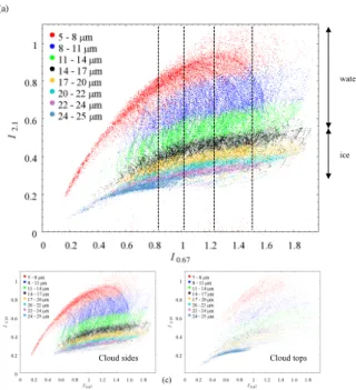
A scatter plot on Fig. 6a is a Nakajima-King (1990) type diagram that relates cloud reflectances at 2.1 and 0.67 µm. The plot is based on 20 cloud fields generated as realizations of the stochastic cloud model described in Sect. 3. In contrast to a

tradi-10

tional Nakajima-King scatter plot that shows only the cloud-top reflectance, most of the points on Fig. 6a correspond to the reflectance from cloud sides. Indeed, panels (b) and (c) illustrate the break down of panel (a) into reflectance from cloud sides and cloud tops, respectively. Panel (b) is much brighter than panel (c), i.e., much more photons have been reflected from cloud sides than from cloud tops. We also see from panel

15

(c) that, since cloud droplet (particle) size increases linearly with height (see, Eq. 3a), only those cloud tops that have the largest r_e=25 µm (blue dots) have substantially contributed to the total reflectance. Because of low VZA (θ=70◦), other cloud tops are in shadow and are barely seen by the observer. As explained in Sect. 2.3, at 2.1 µm the cloud-top reflectances (blue dots) are the smallest. At 0.67 µm, the cloud-top

re-20

flectances have a wide range of values; the latter corresponds to the variety of cloud optical thicknesses as follows directly from the Nakajima-King (1990) theory.

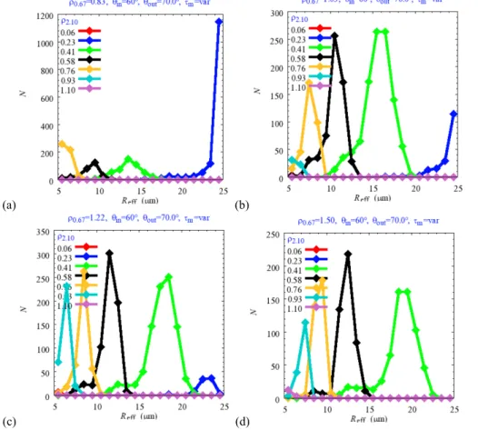
Let us now fix the 0.67 µm reflectances at four different levels (dash lines in Fig. 6a) and build histograms of r_e for different values of the 2.1 µm reflectances. Figure 7 illustrates them (with a window of ±0.03 for I_0.67 and ±0.02 for I_2.1). As expected, for

25

I_0.67=0.83, most observed radiances are reflected from the cloud top with r_e=25 µm.

Increasing I_0.67, we observe more and more radiances reflected from the cloud side. For the large enough 0.67 µm reflectances, I_2.1 saturates and, similar to the plane-parallel approximation, the retrieved values of r_e become insensitive to the values of

(14)

ACPD

6, 7207–7233, 2006

EGU I_0.67. Because of the statistical nature of our retrievals, instead of a single value of

r_e, we retrieve its (conditional) probability density, p(r_e|I_0.67,I_2.1). The mean r_e can be calculated as hr_ei= ∞ Z 0 r_ep( r_e| I_0.67, I_2.1)dr_e (6a)

and its standard deviation σ as

5 σ= v u u u t ∞ Z 0 (r_e− hrei)2p( re| I0.67, I2.1)dre. (6b)

For example, for I_0.67=1.22±0.03 and I_2.1=0.58±0.02, the mean retrieved value

<r_e>=12 µm with standard deviation σ=2 µm.

If, in addition to the measurements at 0.67 and 2.1 µm, one also measures the cloud side brightness temperature, say at 11.6 µm, each retrieved distribution of effective

ra-10

dius can be directly related to cloud side brightness temperature, thus assessing its altitude (for details see the companion paper, Martins et al., 20061). In other words, a combination of measurements at these three wavelengths can resolve the vertical dis-tribution of cloud droplet sizes near cloud side. The extension of the retrieved profiles from cloud sides to the whole cloud requires an additional assumption of mild

fluctu-15

ations of droplet effective radii along a horizontal plane at the same altitude z inside clouds. As discussed in Martins et al. (2006)1, studies of in situ measurements in Cumulus clouds (e.g., Blyth and Latham, 1991) and cloud models (Zev Levin, private communications) confirm that this assumption does not look unrealistic either.

Generally speaking, to retrieve a vertical profile of droplet effective radius, the above

20

approach suggests using a database of stochastic cloud models and corresponding radiative transfer calculations of cloud reflectances at 0.67, 2.1 and 11.6 µm. This is similar to a Bayesian retrieval algorithm (e.g., McFarlane et al., 2002; Evans et al.,

(15)

ACPD

6, 7207–7233, 2006

EGU

2002) that combines prior information about cloud structure and microphysics with ra-diative transfer calculations,

p( x| I_0.67, I_2.1, I_11.6)= p( I0.67, I2.1, I11.6| x)p(x)

R p(I_0.67, I_2.1, I_11.6| x)p(x)d x. (7) Here the vector x consist of cloud parameters (with r_e) that affect the cloud re-flectances: I_0.67, I_2.1and I_11.6. Function p(I_0.67,I_2.1,I_11.6|x) is the conditional probability

5

density function given vectorx. It is directly related to our pre-calculated database –

the radiative transfer simulations of cloud reflectances for the cloud structure defined by

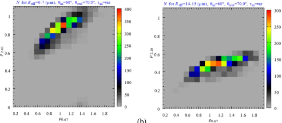
x. Figure 8 shows an example of the conditional probability function of two reflectances I_0.67 and I_2.1for r_e from 6 to 7 µm and from 14 to 15 µm, respectively. Other parame-ters of cloud structure (vectorx) that affect calculations of I_0.67and I_2.1 are described

10

in Sect. 3 and in the caption to Fig. 6. Note that the distribution functions in Fig. 8 are not necessarily Gaussian. Function p(x) is the probability density function of cloud

structure x. In other words, based on the prior information it defines the weights to

be accounted for characterizing the frequency of statex. The integral in the

denom-inator on the right hand side of (7) is just a normalizing factor. Finally, the left hand

15

side of (7) is the (posterior) probability density of having cloud structure x (including r_e) giving measurements of I_0.67, I_2.1 and I_11.6. It is related to histograms shown in Fig. 7. For details on a Bayesian retrieval algorithm applied to microwave radiometer and submillimeter-wave cloud ice radiometer see the excellent descriptions given in McFarlane et al. (2002) and Evans et al. (2002), respectively.

20

5 Summary and discussion

Knowledge on vertical distribution of droplet sizes is essential for understanding not only cloud development and precipitation but also the interactions between clouds and aerosols. Recently Andreae et al. (2004) using in situ aircraft measurements showed a strong dependence of various cloud properties (including droplet sizes), as a function

(16)

ACPD

6, 7207–7233, 2006

EGU

of height in the cloud, on abundance of aerosol particles. How can one obtain this information globally from satellite remote sensing?

For this purpose, a new satellite mission, called CLAIM-3D (stands for “3-D cloud aerosol interaction mission”) has been recently proposed (Martins et al., 20061). The CLAIM-3D mission is designed to advance our understanding of cloud and precipitation

5

development by measuring vertically resolved cloud parameters. It is proposed to have a unique combination of extended wavelength range (0.38–12 µm), polarization, and multi-angle 3-D geometry combining the best features from POLDER (polarization and multi-angle), MISR (multi-angle), and MODIS (multi-channel) to characterize aerosols and cloud microphysics. This paper is the first step towards possible interpretation of

10

CLAIM-3D measurements of reflected from cloud sides solar radiation.

Over the last two decades, considerable efforts have been dedicated to optical remote sensing of cloud properties. Using plane-parallel radiative transfer theory (e.g. Nakajima and King, 1990), measured radiances have been turned into science products, such as cloud optical depth and effective radius. If this approach is

accept-15

able for a stratiform type clouds, it is suspect for clouds that are far from horizontally homogeneous (e.g., Varnai and Marshak, 2001; Iwabuchi and Hayasaka, 2002; Davis, 2002), especially for the clouds with a relatively small aspect ratio (the ratio of horizon-tal to vertical cloud dimensions) and well-developed cloud sides. These are the clouds the CLAIM-3D mission is directed for. In other words, here we target cloud side passive

20

remote sensing rather than traditional cloud top remote sensing.

However, in order to interpret the cloud side measurements, a new 3-D-based cloud retrieval scheme should be developed. Advances in 3-D radiative transfer algorithms, improved understanding of 3-D cloud structure (Marshak and Davis, 2005), and in-creases in computing power make the time now ripe for 3-D cloud retrieval.

25

This paper studies the properties of radiation reflected from cloud sides at two wave-lengths: one nonabsorbing (0.67 µm) and one water-absorbing (2.1 µm). As a proof of concept, it shows that (under some general assumptions and limitations) using Bayesian approach (e.g., Evans et al., 2002) simultaneous measurements of radiances

(17)

ACPD

6, 7207–7233, 2006

EGU

at these two wavelengths can be mapped into a distribution of cloud droplet sizes. Not unlike the famous Nakajima-King (1990) diagram that maps cloud top reflections into a pair of cloud optical depth and effective radius, a new algorithm based on cloud stochastic models is capable in interpreting cloud side reflections at 0.67 and 2.1 µm in terms of cloud droplet size distribution. If the information on cloud side brightness

5

temperature is available, droplet size distributions can be vertically resolved.

Of course, knowledge of reflectance from the pixels surrounding each target pixel as well as reflectance at multiple angles will improve our retrieval making the width of the retrieved distribution narrower. However, to match cases in a simulated retrieval database with cloud side measurements we need to keep the number of parameters

10

describing the relevant information about 3-D cloud structure as few as possible. As the next step, different combinations of radiances in our simulated retrieval database will be tested.

Obviously, the retrieved values of droplet effective radius will correspond to droplets located not far (less than 1 km) from the cloud’s outer walls. However, in situ

obser-15

vations showed that the effective radius may remain constant for any given level in the cloud. In theses cases, retrieving effective radius near the cloud edges will give us information of the microphysics occurring in the cloud’s core. These features are discussed in more details by Martins et al. (2006)1.

Acknowledgements. This work was supported by NASA Goddard Space Flight Center New

20

Opportunities Office. We thank H. Barker, A. Davis, G. Feingold, I. Koren, B. Mayer, L. Remer, T. Varnai and G. Wen for stimulating discussions.

References

Andreae, M. O., Rosenfeld, D., Artaxo, P., Costa, A. A., Frank, G. P., Longo, K. M. , and Silva-Dias, M. A. F: : Smoking rain clouds over the Amazon, Science, 303(5662), 1337–1342,

25

(18)

ACPD

6, 7207–7233, 2006

EGU

Blyth, A. M. and Latham, J.: A climatological parameterization for cumulus clouds, J. Atmos. Sci., 48, 2367–2371, 2001.

Br ´eon F. M. and Goloub, P.: Cloud droplet effective radius from spaceborne polarization mea-surements, Geophys. Res. Lett., 25, 1879–1882, 1998.

Br ´eon, F. M. and Doutriaux-Boucher, M.: A comparison of cloud droplet radii measured from

5

space, IEEE Trans. Geosci. Remote Sens., 4(8), 1796–1805, 2005.

Chang, F.-L. and Li, Z.: Estimating the vertical variation of cloud droplet effective radius us-ing multispectral near-infrared satellite measurements, J. Geophys. Res., 107(D15), 4257, doi:10.1029/2001JD000766, 2002.

Davies, R.: The effect of finite geometry on the three-dimensional transfer of solar irradiance in

10

clouds, J. Atmos. Sci., 35, 1712–1725, 1978.

Davies, R.: Reflected solar radiances from broken cloud scenes and the interpretation of scan-ner measurements, J. Geophys. Res., 89, 1259–1266, 1984.

Davis, A. B.: Cloud remote sensing with sideways-looks: Theory and first results using Mul-tispectral Thermal Imager (MTI) data, in: S.P.I.E. Proceedings, edited by: Shen, S. S. and

15

Lewis, P. E., 4725, S.P.I.E. Publications, Bellingham (Wa), 2002.

Evans, K. F.: The Spherical Harmonics Discrete Ordinate Method for Three-Dimensional At-mospheric Radiative Transfer, J. Atmos. Sci., 55, 429–446, 1998.

Evans, K. F., Walter, S. J., Heymsfield, A. J., and McFarquhar, G. M.: The Submillimeter-wave cloud ice radiometer: Simulations of retrieval algorithm performance, J. Geophys. Res., 107,

20

4028, doi:10.1029/2001JD000709, 2002.

Evans K. F. and Marshak, A.: Numerical Methods in Three-Dimensional Radiative Transfer, in: “Three-Dimensional Radiative Transfer in Cloudy Atmospheres”, edited by: Marshak, A. and Davis, A. B., Springer, 243–282, 2005.

Iwabuchi, H. and Hayasaka, T.: Effects of cloud horizontal inhomogeneity on the optical

thick-25

ness retrieved from moderate-resolution satellite data, J. Atmos. Sci., 59, 2227–2242, 2002. McFarlane, S. A., Evans, K. F., and Ackerman, A. S.: A Bayesian algorithm for the retrieval of liquid water properties from microwave radiometer and millimiter radar data, J. Geophys. Res., 107(D16), 4317, doi:10.1029/2001JD001011, 2002.

Marchuk, G., Mikhailov, G., Nazaraliev, M., Darbinjan, R., Kargin, B., and Elepov, B.: The Monte

30

Carlo Methods in Atmospheric Optics, Springer-Verlag, New-York (NY), 208 pp., 1980. Marshak, A., Davis, A., Cahalan, R. F., and Wiscombe, W. J.: Bounded cascade models as

(19)

ACPD

6, 7207–7233, 2006

EGU

Marshak, A., Davis, A., Wiscombe, W. J., Ridgway, W., and Cahalan, R. F.: Biases in shortwave column absorption in the presence of fractal clouds, J. Climate, 11, 431–446, 1998.

Marshak, A. and Davis, A. B. (Eds): “Three-Dimensional Radiative Transfer in Cloudy Atmo-spheres”, Springer, 686 p., 2005.

McKee, T. B. and Cox, S. K.: Scattering of visible radiation by finite clouds, J. Atmos. Sci., 31,

5

1885–1892, 1974.

Nakajima, T. Y. and King, M. D.: Determination of the optical thickness and effective particle radius of clouds from reflected solar radiation measurements – Part I, Theory, J. Atmos. Sci., 47, 1878–1893, 1990.

Platnick S.: Vertical photon transport in cloud remote sensing problems, J. Geophys. Res., 105,

10

22 919–22 935, 2000.

Platnick, S., King, M. D., Ackerman, S. A., Menzel, W. P., Baum, B. A., Riedi, J. C., and Frey, R. A.: The MODIS cloud products: Algorithms and examples from Terra, IEEE Trans. Geosci. Remote Sens., 41(2), 459–473, 2003.

Prigarin, S. and Marshak, A.: Numerical model of broken clouds adapted to observations,

15

Atmos. Oceanic Optics, 18, 256–263, 2005.

Ramanathan, V., Crutzen, P. J., Kiehl, J. T., and Rosenfeld, D.: Aerosols, climate and the hydrological cycle, Science, 294, 2119–2124, 2001.

Rosenfeld, D.: Suppression of rain and snow by urban and industrial air pollution, Science, 287, 1793–1796, 2000.

20

Rosenfeld, D. and Ulbrich, C. W.: Deep convective clouds with sustained supercooled liquid water down to −37.5◦C, Nature, 405, 440–442, 2000.

Schertzer, D. and Lovejoy, S.: Physical modeling and analysis of rain and clouds by anisotropic scaling multiplicative processes, J. Geophys. Res., 92, 9693–9714, 1987.

Stamnes, K., Tsay, S.–C., Wiscombe, W. J., and Jayaweera, K.: Numerically stable algorithm

25

for discrete-ordinate-method radiative transfer in multiple scattering and emitting layered me-dia, Appl. Opt., 27, 2502–2512, 1988.

Stephens, G. L.: Remote Sensing of the Lower Atmosphere. An Introduction, Oxford University Press, pp. 523, 1994.

Stephens, G. L., Vane, D. Boain, R., Mace, G., Sassen, K., Wang, Z., Illingworth, A., O’Connor,

30

E., Rossow, W., Durden, S., Miller, S., Austin, R., Benedetti, A., Mitrescu, C., and CloudSat Science Team: The CloudSat mission and the A-Train: A new dimension of space-based observations of clouds and precipitation, Bull. Amer. Metereol. Soc., 83, 1771–1790, 2002.

(20)

ACPD

6, 7207–7233, 2006

EGU

V ´arnai, T. and Marshak, A.: Observations and analysis of three-dimensional radiative effects that influence MODIS cloud optical thickness retrievals, J. Atmos. Sci., 59, 1607–1618, 2002.

(21)

ACPD

6, 7207–7233, 2006

Printer-friendly Version Interactive Discussion EGU Figures (a) 0 12.8 km 2 km Sun !0=60o Cloud top Cloud side Satallite ! (b) 0 0.5 1 1.5 2 -5.0 0.0 5.0 10.0 ra d ia n c e x (km) 0.67 µm 2.1 µm !=80 !=40 !=20 !=80 !=40 !=20 !=160 !=160 Cloud top Cloud side (c) 0 0.4 0.8 1.2 1.6 -5.0 0.0 5.0 10.0 ra d ia n c e x (km) !=60o 2.1 µm !=70o 0.67 µm !=60o !=45o !=45o Cloud top Cloud side

Figure 1. Reflectance from a single cloud at two wavelengths: 0.67 µm (solid symbols) and 2.1 µm (empty symbols). Cloud height h = 2 km, cloud width L = 12.8 km, droplet effective radius, re = 10 µm, SZA θ0=60ο (a) A

schematic illustration of illumination and viewing angles. Negative x correspond to reflectances from ‘cloud side’ while positive x correspond to reflectances from ‘cloud top’; (b) θ = 60ο_{; cloud optical thickness τ = 160, 80, 40 and 20; (c)}

τ = 80, θ = 70ο_{, 60}ο_{, and 45}ο_.

Fig. 1. Reflectance from a single cloud at two wavelengths: 0.67 µm (solid symbols) and

2.1 µm (empty symbols). Cloud height h=2 km, cloud width L=12.8 km, droplet effective radius,

r_e=10 µm, SZA θ₀=60◦(a) A schematic illustration of illumination and viewing angles. Negative

x correspond to reflectances from “cloud side” while positive x correspond to reflectances from

“cloud top”;(b) θ=60◦; cloud optical thickness τ=160, 80, 40 and 20; (c) τ=80, θ=70◦, 60◦and 45◦.

(22)

ACPD

6, 7207–7233, 2006

Printer-friendly Version Interactive Discussion EGU 20 (a) (b)

Figure 2. Reflectance from a single cloud with a variable droplet effective radius. Cloud height h = 4 km, cloud size

L = 6.5 km, flat cloud top, τ = 80, θo = 60o, θ = 45o. Droplet effective radius re increases linearly with height from 5

to 25 µm. (a) 0.67 µm; (b) 2.1 µm. Cloud edge is indicated by arrow at x = 7.5 km. Reflectance from cloud top is at the right side from the cloud edge while reflectance from cloud side is at the left. Dots indicate ‘measurements’ at s = 0.25 km resolution. Cloud edge Cloud edge Cloud top Cloud side I0.67 I2.1

Fig. 2. Reflectance from a single cloud with a variable droplet effective radius. Cloud height

h= 4 km, cloud size L=6.5 km, flat cloud top, τ=80, θ_o= 60◦, θ=45◦. Droplet effective radius re

increases linearly with height from 5 to 25 µm. (a) 0.67 µm; (b) 2.1 µm. Cloud edge is indicated

by arrow at x=7.5 km. Reflectance from cloud top is at the right side from the cloud edge while reflectance from cloud side is at the left. Dots indicate “measurements” at s=0.25 km resolution.

(23)

ACPD

6, 7207–7233, 2006

EGU (a)

(b)

Figure 3. A realization of cloud stochastic model that has a given power-spectral exponent, mean, and standard

deviation. (a) optical depth filed; (b) cloud top height field.

Fig. 3. A realization of cloud stochastic model that has a given power-spectral exponent, mean,

and standard deviation. (a) optical depth filed; (b) cloud top height field.

(24)

ACPD

6, 7207–7233, 2006

EGU

22

Figure 4. An example of cloud microphysics. (a) liquid water content, LWC; (b) number of drops, N; (c) droplet

effective radius, re; (d) extinction coefficient, σext.

(a)

(b)

(c)

(d)

22

(a)

(b)

(c)

(d)

22

(a)

(b)

(c)

(d)

22

(a)

(b)

(c)

(d)

Fig. 4. An example of cloud microphysics. (a) liquid water content, LWC; (b) number of drops,

N; (c) droplet effective radius, re; (d) extinction coefficient, σext.

(25)

ACPD

6, 7207–7233, 2006

EGU

23

Figure 5. Reflectance from a realization of a stochastic cloud model with constant cloud optical (τ=80) and geometrical

thicknesses (h=4 km). Left column: 0.67 µm; right column: 2.1 µm; θ0=60

o_{; θ=0}o_{, 20}o_{, 45}o_{, and 70}o_{, from top to}

bottom. Note different color scales for left and right columns.

Fig. 5. Reflectance from a realization of a stochastic cloud model with constant cloud optical

(τ=80) and geometrical thicknesses (h=4 km). Left column: 0.67 µm; right column: 2.1 µm;

θ0=60◦; θ=0◦, 20◦, 45◦, and 70◦, from top to bottom. Note different color scales for left and right columns.

(26)

ACPD

6, 7207–7233, 2006

EGU

24

(a)

Figure 6. A scatter plot of 2.1 µm reflectances vs. 0.67 µm reflectances based on 20 cloud fields generated by stochastic cloud model described in section 3. Parameters of the model are the following: mean cloud optical thickness = 80, mean cloud height = 4 km, spectral exponent = 2.0, standard deviations = 16 for the optical thickness and 1 km for the cloud height, cloud fraction = 0.5, θ0=60o, θ=70o. Particles smaller than 15 µm are water droplets while

particles larger than 15 µm are ice. (a) Reflectances from both cloud sides and cloud tops. Dash lines indicate fixed 0.67 µm reflectances (±0.03) used in Fig. 7. (b) Reflectance from cloud sides. (c) Reflectance from cloud tops.

Cloud sides Cloud tops water

ice

(b) (c)

Fig. 6. A scatter plot of 2.1 µm reflectances vs. 0.67 µm reflectances based on 20 cloud fields

generated by stochastic cloud model described in Sect. 3. Parameters of the model are the following: mean cloud optical thickness= 80, mean cloud height = 4 km, spectral exponent = 2.0, standard deviations = 16 for the optical thickness and 1 km for the cloud height, cloud fraction= 0.5, θ₀=60◦, θ=70◦. Particles smaller than 15 µm are water droplets while particles larger than 15 µm are ice. (a) Reflectances from both cloud sides and cloud tops. Dash lines

indicate fixed 0.67 µm reflectances (±0.03) used in Fig. 7. (b) Reflectance from cloud sides. (c) Reflectance from cloud tops.

(27)

ACPD

6, 7207–7233, 2006

EGU

(a) (b)

(c) (d)

Figure 7. Histograms (number of cases vs. effective radius) obtained from Fig. 6. Values of reflectance at 0.67 µm

were set to 0.83, 1.03, 1.22, and 1.50 with a ±0.03 window, on panels (a), (b) (c) and (d) respectively. Values of reflectance at 2.1 µm have a ±0.02 window.

Fig. 7. Histograms (number of cases vs. effective radius) obtained from Fig. 6. Values of

reflectance at 0.67 µm were set to 0.83, 1.03, 1.22, and 1.50 with a ±0.03 window, on panels

(a), (b) (c) and (d) respectively. Values of reflectance at 2.1 µm have a ±0.02 window.

(28)

ACPD

6, 7207–7233, 2006

EGU

(a) (b)

Figure 8. Histograms of reflectances at 0.67 µm and 2.1 µm conditional the effective radius equal to (a) 6-7 µm and (b) 14-15 µm. Plot is based on 20 realizations of the stochastic cloud model described in section 3. Parameters of the

model are the same as in Fig. 6.

Fig. 8. Histograms of reflectances at 0.67 µm and 2.1 µm conditional the effective radius equal

to(a) 6–7 µm and (b) 14–15 µm. Plot is based on 20 realizations of the stochastic cloud model

described in Sect. 3. Parameters of the model are the same as in Fig. 6.