Nouvelles approches de tomographies hydrauliques en aquifère hétérogène : théories et applications en milieu karstique et fracturé.

HAL Id: tel-01955328

https://tel.archives-ouvertes.fr/tel-01955328

HAL is a multi-disciplinary open access archive for the deposit and dissemination of sci-entific research documents, whether they are pub-lished or not. The documents may come from teaching and research institutions in France or abroad, or from public or private research centers.

L’archive ouverte pluridisciplinaire HAL, est destinée au dépôt et à la diffusion de documents scientifiques de niveau recherche, publiés ou non, émanant des établissements d’enseignement et de recherche français ou étrangers, des laboratoires publics ou privés.

aquifère hétérogène : théories et applications en milieu

karstique et fracturé.

Pierre Fischer

To cite this version:

Pierre Fischer. Nouvelles approches de tomographies hydrauliques en aquifère hétérogène : théories et applications en milieu karstique et fracturé.. Sciences de la Terre. Normandie Université, 2018. Français. �NNT : 2018NORMR059�. �tel-01955328�

THÈSE

Pour obtenir le diplôme de doctorat

Préparée au sein de l’Université de Rouen Normandie

Nouvelles approches de tomographies hydrauliques en aquifère hétérogène

Présentée et soutenue par

Pierre FISCHER

Thèse dirigée par Abderrahim JARDANI et Nicolas LECOQ, laboratoire Morphodynamique Continentale et Côtière (M2C)

Thèse soutenue publiquement le 21 novembre 2018 devant le jury composé de

Mr Frederick DELAY Pr / LHyGeS / Université de Strasbourg Rapporteur

Mr Olivier BOUR Pr / Géosciences Rennes / Université de

Rennes 1 Rapporteur

Mr Philippe RENARD DR / CHYN / Université de Neuchâtel Rapporteur

Mr André REVIL DR / ISTerre / Université Grenoble Alpes Examinateur

Mme Mickaële LE RAVALEC DR / IFPEN Rueil-Malmaison Examinatrice

Mr Michel QUINTARD DR / IMFT / Université Toulouse 3 Examinateur

Mr Abderrahim JARDANI MCF HDR / M2C / Université de Rouen

Normandie Directeur de thèse

Mr Nicolas LECOQ MCF HDR / M2C / Université de Rouen

Nouvelles approches de tomographies hydrauliques en aquifère

hétérogène

Théories et applications en milieu karstique et fracturé

New hydraulic tomography approaches in heterogeneous aquifer

par

Pierre FISCHER

Manuscrit de thèse rédigé et présenté en vue d’obtenir le diplôme de doctorat

SpécialitéSciences de l’Univers

Thèse préparée au sein de l’Université de Rouen Normandie 2018

R

ÉSUMÉ

Ce manuscrit de thèse présente une nouvelle approche pour caractériser qualitativement et quantitativement la localisation et les propriétés des structures dans un aquifère fracturé et karstique à l’échelle décamétrique. Cette approche est basée sur une tomographie hydraulique menée à partir de réponses à une investigation de pompages et interprétée avec des méthodes d’inversions adaptées à la complexité des systèmes karstiques. L’approche est appliquée sur un site karstique d’étude expérimental en France, une première fois avec des signaux de pompage constants, et une deuxième fois avec des signaux de pompage harmoniques. Dans les deux cas, l’investigation a fourni des réponses de niveaux d’eau de nappe mesurés pendant des pompages alternés à différentes positions. L’interprétation quantitative de ces jeux de réponses consiste à les reproduire par un modèle avec un champ de propriété réaliste adéquat généré par inversion. Les méthodes d’inversions proposées dans ce manuscrit permettent de reconstruire un champ de propriétés hydrauliques réaliste en représentant les structures karstiques soit par un réseau généré par automates cellulaires, soit par un réseau discrétisé. Les résultats d’interprétations obtenus sur le site d’étude expérimental permettent d’imager les structures karstiques sur une carte et de « lire » leur localisation. De plus, les résultats obtenus avec les réponses à des pompages harmoniques tendent à montrer le rôle de la fréquence du signal sur les informations portées par les réponses. En effet, les fréquences plus élevées caractérisent mieux les structures les plus conductrices, alors que les fréquences plus faibles mobilisent des écoulements également dans des structures karstiques moins conductrices.

A

BSTRACT

This thesis manuscript presents a novel approach to characterize qualitatively and quantitatively the structures localization and properties in a fractured and karstic aquifer at a decametric scale. This approach relies on a hydraulic tomography led from responses to a pumping investigation and interpreted with inversion methods adapted to the complexity of karstic systems. The approach is applied on a karstic experimental study site in France, a first time with constant pumping signals, and a second time with harmonic pumping signals. In both applications, the investigation resulted in groundwater level responses measured during alternated pumping tests at different locations. The quantitative interpretation of these sets of responses consists in reproducing these responses through a model with an adequate realistic property field generated by inversion. The inversion methods proposed in this manuscript permit to reconstruct a realistic hydraulic property field by representing the karstic structures either through a network generated by cellular automata, or through a discretized network. The interpretation results obtained on the experimental study site permit to image the karstic structures on a map and to ‘read’ their localization. Furthermore, the results obtained with the responses to harmonic pumping tests tend to show the role of the signal frequency on the information carried by the responses. In fact, higher frequencies better characterize the most conductive structures, while lower frequencies mobilize flows also in less conductive karstic structures.

R

EMERCIEMENTS

Je vais commencer par remercier, dans cette partie, mes directeurs de thèses, Abderrahim Jardani et Nicolas Lecoq. Merci de m’avoir fait confiance, dès le début, en me prenant en doctorant sans m’avoir vraiment réellement rencontré et en montant un financement non forcément prévu à la base. Merci également pour la confiance et la liberté accordée durant ma thèse qui m’ont permis de publier des articles, et notamment sur un concept que je voulais y développer, les automates cellulaires. Ensuite je vais remercier les autres membres de mon jury, André Revil, Frederick Delay, Olivier Bour, Philippe Renard, Mickaële Le Ravalec et Michel Quintard. Merci d’avoir accepté de lire mon manuscrit, d’avoir assisté à ma présentation de soutenance et d’avoir discuté, commenté et critiqué mes travaux afin de me montrer de nouvelles perspectives.

Mes prochains remerciements, plus personnels, iront à mes proches et membres de ma famille. Tout d’abord merci ma chérie Louise, pour m’avoir soutenu tout le long de ce doctorat. Tu m’as d’abord encouragé dans la période de transition entre la fin de mon TFE et le début du doctorat 10 mois après. Tu m’as suivi à Rouen malgré la difficulté à y trouver un travail. Puis tu m’as soutenu, apaisé et parfois secoué dans les hauts et les bas de ces trois années. Enfin tu m’as grandement aidé dans la dernière ligne droite pour organiser toute ma journée de soutenance. Pour tout ça je te remercie, mais aussi plus généralement pour tout le bonheur que tu m’as apporté. Il n’y a pas une seule seconde depuis qu’on est ensemble durant laquelle l’amour que j’ai pour toi et la fierté de t’avoir comme compagne n’a cessé de grandir.

Merci à mes parents, Christine et Gottfried, pour m’avoir soutenu dans l’idée de réaliser un doctorat et d’être régulièrement venu nous rendre visite à Rouen. Merci également pour l’aide apportée à la réalisation de mon pot de soutenance. Merci à mes grands frères, Julien et Stephan, pour m’avoir « ouvert la voie » dans le système éducatif et avoir influencé mes différentes décisions de formations. Merci Stephan pour tes nombreux conseils, ton aide précieuse quand j’en avais besoin, d’être venu des Etats-Unis pour ma soutenance, et pour les games de LoL épiques les week-ends. Merci à mes autres proches qui se sont déplacés pour assister à ma soutenance, Mamie, Papi, Laurence, Agnès et Jacques. Je remercie également Oma et Opa, qui ne pouvaient malheureusement pas se déplacer pour ma soutenance mais qui ont eu l’occasion de m’adresser tous leurs encouragements.

Merci enfin aux autres membres de mes proches (plus particulièrement Marie-Christine, Nicole, Guillaume, Ysabault, Charlotte) pour leur constante bienveillance envers moi et leurs encouragements tout au long de mon doctorat. Pour finir, merci Snow, même si tu ne sais pas (encore) lire, je suis sûr que tu apprécieras au moins mes papouilles.

Ensuite, je vais remercier les autres personnes qui m’ont accompagné, de près ou de loin durant ces trois années de doctorat. Je commencerai par remercier les doctorants que j’ai régulièrement côtoyé au labo M2C « antenne de Rouen ». Merci Arnaud, Aziz, Théo, Manu, Flavie, Marie, Antonin, Thomas, Adeline, David, Mohamad, Nazih, Ruth, Manon, Mickaël, Léa, Valentin, Edward, Antoine, Raphaël. Merci à cette « ligue de doctorants extraordinaires », très soudée et joviale, qui aura grandement participé à rendre mes trois années de doctorats très agréables, que ce soit au labo durant les passionnants et passionnés échanges du repas du midi, ou dans les nombreuses soirées.

Je remercie également les membres permanents du labo. Merci d’abord à Michel, pour ton aide sur la préparation et la réalisation de ma campagne de terrain, mais également évidemment pour ta bonne humeur que tu apportes au labo. Merci également à Abderrahim, Nicolas L., Jean-Paul (avec une pensée particulière), Maria, Nicolas M., Matthieu, Robert, Julien, Maxime et Yoann, pour vos conseils et l’aide que vous avez pu régulièrement m’apporté en colloque ou au labo. Merci à tous les autres membres du labo pour votre accueil qui m’a fait me sentir bien au sein du laboratoire (à tel point que je me suis mis à m’y promener en chaussettes).

Je vais finir par remercier les personnes qui m’ont décidé à faire un doctorat et celles qui m’ont aidé à le réaliser. Merci Fabrice Golfier pour le projet de Master qui m’a appris et donné le goût des modèles et de la recherche. Merci David Labat de m’avoir fait découvrir les karsts et leurs études. Merci Hervé Jourde pour l’aide apportée sur les applications de mes méthodes sur le site du Terrieu. Merci Michael Cardiff pour l’aide apportée sur les modèles fréquentiels et les signaux harmoniques. Merci enfin à tous mes autres co-auteurs, Xiaoguang, Stéphane, Mohamad, Abdellahi, pour leurs aides et leurs corrections sur mes articles.

S

OMMAIRE

Liste des figures 10

Liste des tableaux (tables) 20

1 Introduction générale 23

2 Tomographie hydraulique en milieu alluvial avec inversion géostatistique 37

2.1 Contexte 39

2.2 Application of large-scale inversion algorithms to hydraulic tomography in

an alluvial aquifer 41

2.2.1 Introduction 42

2.2.2 Principal component geostatistical approach 45

2.2.3 Application to an experimental site 49

2.2.4 Results 52

2.2.5 Conclusion 61

3 Un nouvel outil d'inversion structurale pour les modèles équivalents milieux poreux 63

3.1 Contexte 65

3.2 A cellular automata-based deterministic inversion algorithm for the

characterization of linear structural heterogeneities 67

3.2.1 Introduction 68

3.2.2 Parameterization of inverse problem using cellular automaton 70

3.2.3 Optimization process 81

3.2.4 Applications 85

3.2.5 Discussion and conclusion 99

4 Un nouvel outil d'inversion structurale pour les modèles discrets couplés 103

4.1 Contexte 105

4.2 Hydraulic tomography of discrete networks of conduits and fractures in a

karstic aquifer by using a deterministic inversion algorithm 107

4.2.1 Introduction 108

4.2.2 Algorithm framework 111

4.2.3 Validation of the DNDI algorithm on hypothetical study cases 121

4.2.4 Discussion 130

4.2.5 Conclusion 131

5 Caractérisation des écoulements dans le site du Terrieu par pompage à débit

constant 135

5.1 Contexte 137

5.2 Identifying flow networks in a karstified aquifer by application of the

cellular automata-based deterministic inversion method (Lez aquifer, France) 139

5.2.1 Introduction 140

5.2.2 Methodology 142

5.2.3 Application 148

6 Analyse hydraulique des réponses à un pompage harmonique en milieu

karstique et fracturé 163

6.1 Contexte 165

6.2 Hydraulic Analysis of Harmonic Pumping Tests in Frequency and Time

Domains for Identifying the Conduits Networks in a Karstic Aquifer 167

6.2.1 Introduction 168

6.2.2 Theoretical background 171

6.2.3 Synthetic application 175

6.2.4 Example of harmonic pumping investigation 189

6.2.5 Discussion and conclusion 195

7 Application de tomographie hydraulique en mode harmonique sur le site du Terrieu 199

7.1 Contexte 201

7.2 Harmonic Pumping Tomography Applied to Image the Hydraulic Properties and Interpret the Connectivity of a Karstic and Fractured

Aquifer (Lez Aquifer, France) 203

7.2.1 Introduction 204 7.2.2 Field investigation 207 7.2.3 Modeling methodology 215 7.2.4 Modeling application 223 7.2.5 Discussion 237 7.2.6 Conclusion 239

8 Conclusion générale et perspectives 241

Bibliographie (References) 251

L

ISTE DES FIGURES

Figure 1.1: Gauche : Répartition des grands hydrosystèmes souterrains français (BRGM 2015). Droite : Répartition des formations karstifiables en France

(Marsaud 1996). 26

Figure 1.2: Schématisation des écoulements dans trois types de milieux pouvant être aquifère : milieux poreux, fracturés et karstiques (modifié d’après

Heath 1998). 26

Figure 1.3: Schéma de la caractérisation des propriétés par interprétation des

réponses à un signal de sollicitation. 27

Figure 1.4: Représentation schématisée d’une investigation par pompage avec débit à signal constant d’un aquifère fracturé et karstique (modifié d’après Goldscheider

et Drew 2007). 28

Figure 1.5: Schéma de la reconstitution des propriétés à partir d’un modèle direct

et de l’inversion des réponses mesurées. 30

Figure 1.6: Schéma entre la liberté attribuée dans la reconstitution des réponses

dans le processus d’inversion par rapport aux contraintes établies sur les solutions. 31 Figure 1.7: Haut : Schéma des différentes techniques de modélisation distribuées

issu de Ghasemizadeh et al. 2012 (EPM = Equivalent Milieu Poreux ; DPM = Milieu Double Porosité ; DFN = Réseau de Fractures Discrètes ; DCN = Réseau de Conduits Discrets ; HM = Modèle Hybride). Bas : Exemples de modélisations d’aquifères karstiques par (a) EPM (Saller et al. 2013), (b) DPM

(Kordilla et al. 2012), et (c) HM (Kovacs 2003). 32

Figure 2.1: Location of the studied experimental site 'La Céreirède' (Map and aerial photography from geoportail.fr) occupying an area of 720 m². It is situated in

the South of France, near the town of Montpellier and the Mediterranean Sea. 49 Figure 2.2: Schematic geological section of the experimental site ‘La Céreirède’.

Three aquifers formations have been characterized in the sands and silts alluvium,

in the gravels and in the clayey sands. 50

Figure 2.3: Well pattern on the experimental site ‘La Céréirède’ (circles represent the 10 measurement wells and triangles represent the 2 pumping wells). As hydraulic drawdowns in the pumping wells are not measured, the tomography

provided 20 observed data. 51

Figure 2.4: Maps of the log-transmissivity (a, on the left) and parameter’s a posteriori standard deviation (b, on the right) for a PCGA inversion method with 25,600

parameters, 20 observed data and a covariance matrix decomposition of order K=128 applied to the experimental site. The transmissivities vary around a mean of

10-5 _{m²/s which is consistent with transmissivity values estimated from pumping test} analysis. The aquifer is less transmissive in the eastern part and more in the

western part especially in a zone around PZ 7 (see Figure 2.3). But we got a better precision in zones with more information: at the center and the western part of the

map, while in the eastern part where we didn’t have piezometers, the results show

a larger standard deviation. 53

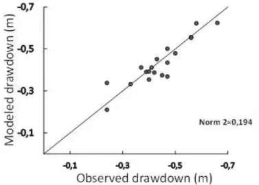
Figure 2.5: Graph showing the differences between the 20 observed drawdowns and modeled drawdowns after convergence of a PCGA inversion method with 25,600 parameters and a covariance matrix decomposition of order K=128 applied to the

experimental site. The drawdowns are globally well reproduced. 54 Figure 2.6: Covariance matrix singular values decrement curve for 10,000 parameters. Three decomposition order (a to c) corresponding to truncation error of 1, 0.1 and 0.01 have been chosen for the results comparison of the PCGA inversion method (see

0.02 Figure 2.7). 55

Figure 2.7: Maps of the log-transmissivity for a PCGA inversion method with 10,000 parameters, 20 observed data and three different covariance matrix

decomposition applied to the experimental site. The map (a) was obtained for K=69, the map (b) for K=313 and the map (c) for K=1,532 (see Figure 2.6). The results obtained for these three decomposition are relatively the same (same transmissivity values, same zones) so, for this site, there is no significant loss of information when using a truncation order corresponding to an error of 1 (map (a)) for the covariance matrix which allows us to reduce the computation time of the inversion without

decreasing the accuracy of the results. 56

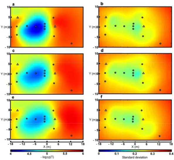
Figure 2.8: Maps of the log-transmissivity (a, c, e) and parameter’s a posteriori standard deviation (b, d, f) for three different inversion methods with 10,000

parameters and 20 observed data applied to the experimental site. The maps (a) and (b) were obtained with the GA adjoint-state method, the maps (c) and (d) with the GA finite-difference method and the maps (e) and (f) with the PCGA method with a covariance matrix decomposition of order K=69. The results between the three methods are relatively the same for this site, except for the map a which presents a slightly higher contrast of the transmissivity distribution leading to a better data matching (see Figure 2.9), though the PCGA inversion method is much more

efficient for the calculation time (see Table 2.2). 57

Figure 2.9: Graphs showing the differences between the 20 observed drawdowns and modeled drawdowns after convergence of three different inversion methods with 10,000 parameters applied to the experimental site. The graph (a) was obtained with the GA adjoint-state method, the graph (b) with the GA finite-difference method and the graph (c) with the PCGA method with a covariance matrix decomposition of order

K=69. Regarding the mathematical norm 2 the GA adjoint-state method has a slightly

better convergence on the data than the other methods but the PCGA inversion

method is much more efficient for the calculation time (see Table 2.2). 59 Figure 3.1: Scheme explaining how the CA are used in the CADI model. In the

figure grey occurs for state ‘background’ and white for state ‘structure’. The model is partitioned in mCA independent CA subspaces (here mCA=9). During the generation process the structure will go through different CA subspaces (a) and will be

generated in the local direction assigned by the structural parameters piloting these CA (b). Along the generation direction the CA will modify the property values of the model cells it controls (represented by the squares lattice in Figure 3.1c). 70 Figure 3.2: An example of the dual-radius neighborhood considered in our CA

definition. The black highlighted cell is the cell under consideration in this example (each cell of the lattice would alternatively be considered during a full CA time

which permit the configuration of the neighborhood. In this example, the inner circle has a radius = 2 and the outer circle has a radius = 3. Additionally, the neighborhood is split into 2

´

configurable weighting definition (see Figure 3.4). 73

Figure 3.3: Time evolution of a CA configured with a neighborhood weighting

defining a horizontal structure generation (see Figure 3.4). After the sixth time step the CA has converged and its geometry is stable over the following steps. Here grey

occurs for state ‘background’ and white for state ‘structure’. 74 Figure 3.4: Presentation of 8 different stable structures started by a unique centered cell, and their associated CA neighborhood configuration. The greyed cell in the neighborhood configuration is a given cell considered during the CA process. It is surrounded by its neighbor cells, which are not shown for reasons of

readability. Its neighborhood is split in 8 internal ‘activator’ sectors and 8 external ‘inhibitor’ sectors, each one being assigned to a given weight. A ‘++’ occurs for a positive weight for the neighbor cells in the area, a ‘++’ weight is twice higher than a positive weight represented by a single ‘+’. A ‘- -‘ occurs for a negative weight for the neighbor cells in the area, a ‘- -‘ weight is twice higher than a negative weight

represented by a single ‘-‘. An empty part of the neighborhood occurs for a null weight, meaning that cells in the area are not considered in the transition rule. Here we present the CA configuration leading to 8 different structure directions

which will be considered as sub-orientation of the global structure in the model. In the structural map, grey occurs for state ‘background’ and white for state ‘structure’. 75 Figure 3.5: Operating scheme for the Cellular Automata-based Deterministic Inversion (CADI) algorithm. After an initialization of PN and Pβ with chosen directions and

property values for each subspace, the algorithm begins an iterative process. It will firstly optimize the geometry of the structure in the model by iteratively

updating the structural model using the CA generation process. Once the objective function has converged to a local minimum on the structure, it will lead a second optimization on the values of the properties for the previously inverted structure, until the objective function converges to a local minimum again. Finally, the

uncertainties on the structure and the properties of the model are estimated. 80 Figure 3.6: Presentation of the 4 different structures tested in the 6 study cases in this paper. The case 1 is a linear inversion of a simple geometry (a) to show how the optimization works. The case 2 is a linear inversion of a more complex geometry (b). The case 3 is a linear inversion of a complex multi-directional linear structure (c). The cases 4, 5 and 6 are linear, non-linear and joint inversion of a geostatistical

generated geometry (d), appearing as a more natural structure. 86 Figure 3.7: Result of the linear inverse modeling of the case study 1. The inversion finished after 4 iterations. This figure shows all different iterations of the inversion, from initial model (a), to inverted model (e). The true structure is shown in (f). The figure (d) corresponds to the structural optimization and the figure (e) to the properties optimization for this structure. The different CA subspaces of the

model are highlighted by the black lines. 87

Figure 3.8: Comparison of the optimal structure found by inversion (in white) and the true structure (bold boundaries) for the case study 1. For this simple geometry, the

inverse algorithm could easily reproduce the structure. 88

Figure 3.9: Result of the linear inverse modeling of the case study 2. The

convergence is performed with 21 iterations. This figure shows some different iterations of the inversion, from initial model (a), to inverted model (e). The true structure is shown in (f). We noted that the optimization on the property values permits to

balance the structural inversion errors. For example, in this case, the structural

additions in the center of the model in (e) were optimized by a light augmentation of its

seismic velocity (0.5 km/s instead 0.26 km/s). 89

Figure 3.10: Comparison of the optimal structure found by inversion (in white) and the true structure (bold boundaries) for the case study 2. The optimization process reproduced a good structural inversion. The few inversion errors in the center of the model were lightly balanced by the inversion on the properties (see Figure 3.9). 90 Figure 3.11: Results of the linear inverse modeling of the case study 3. This figure

shows two inversions with different initial models (a and d), their results (b and e) and the comparison of these results to the true geometry boundaries in red (c and f). The convergence is performed with 26 iterations in the first inversion and 30 iterations in the second. We noted that the information contained in the initial model could slightly modify the result of the inversion but even with a very simple initial case (a) the optimization process permits to find the main shapes and trends of

the true structure (c). 92

Figure 3.12: Map of the positioning of the wells for the hydraulic tomography inversion for the study case 4. The circles are the position of the measurement piezometers

and the triangles are the position of the pumping wells. 92

Figure 3.13: Result of the non-linear inverse modeling of the study case 4. The

inversion finished after 7 iterations. This figure shows the initial model (a), the inverted model (b) and the true structure (c). The inversion process found an optimized

equivalent structure to the initial property value. The true transmissivities were found

during the properties optimization. 93

Figure 3.14: Result of the linear inverse modeling of the study case 5. The inversion finished after 4 iterations. This figure shows the initial model (a), the inverted model (b) and the true structure (c). The structural optimization was limited by the initial properties and by its constant aperture generation to reproduce a variable

aperture true structure. In this case, the optimization on the property values permits to balance the initial information and the structural inversion aperture limitations. The properties optimization balanced this limitation by globally decreasing the seismic

velocity of the background to a lower value than the true one. 94 Figure 3.15: Result of the joint inverse modeling of the study case 6. The inversion finished after 7 iterations. This figure shows the hydraulic model (a), the seismic model (c) and the true models (b,d). The geometry of the structure in the models was

optimized through a joint inversion of seismic and hydraulic data. 96 Figure 3.16: Pixel-wise comparison of the optimal structures found by inversion (in

white) and the true structure (bold boundaries) for the study cases 4 (a), 5 (b) and 6 (c). Both hydraulic and seismic data permitted to find a geometry of the global trends of the true structure but the joint inversion resulted to a better model regarding the structure and also the convergence on the data, which avoided the difficulties

encountered by the simple hydraulic inversion and the simple seismic inversion. 96 Figure 3.17: Uncertainties analysis for the joint inversion of the study case 6. The

structural constraint in (a) indicates where the structure of the model is well-

constrained by a low value, and at the opposite, a high value indicates an uncertainty for its subspace direction. The properties uncertainties for (b) the hydraulic

transmissivity and (c) the seismic velocity are quantified by a standard deviation on

Figure 4.1: Example of a simulated distribution of hydraulic heads (here drawdowns) by solving the forward problem f (Equation (4.1)) for a steady state pumping in a given coupled discrete-continuum distributed model G

(

)

with six subspaces. An activated node in the top subspaces (a) starts the generation of the structure. The structure generates to the nodes in the bottom of these

subspaces, following the local direction defined in the subspaces through the encoding rules. These reached nodes then become activated (b). The subspaces in which the structure has generated become inhibited to another generation (shown as greyed number in this figure). The structure then continues its generation from its newly

activated node if the subspaces structural parameters permit it (c) – (d). 113 Figure 4.3: Parameterization of a model in the DNDI method. For each subspace of the model there are six local direction possibilities (see encoding in Figure 4.2) that are used to parameterize a network structure in the model (a). The structure (in red) is then generated, following a node-to-node rule, from the set of structural parameters in (a) and a chosen starting point at a node between subspaces (b). Finally a set of property values (transmissivities), also defined for each subspace, is assigned to the

structural model (c). 114

Figure 4.4: A flowchart of the inversion steps used in the DNDI algorithm. After the initialization of the parameters, a sequential iterative optimization is led on the structure geometry and on the property values in order to minimize both objective functions (Equations (4.5) and (4.6)). An eventual re-run of the inversion process (multi-scale option) using the result as new initial model can be performed in order to

improve this result. 118

Figure 4.5: Initial and inverted models for an inversion using drawdown data produced from a true model (on the right) with a homogeneous matrix. The red dots on the true model symbolize the pumping/measurement boreholes for the hydraulic data. The inverted model permits to localize approximatively the karstic network connections but in this case the amount of data is insufficient to have a proper imagery. 123 Figure 4.6: Initial (a) and inverted (b) models for an inversion using drawdown data

produced from a true model with a homogeneous matrix, and associated map of the conduit properties posterior standard deviations (c). The inverted model in (b) permits a good localization the true karstic network. It also reduced locally the initial

transmissivity (0.06 m²/s to 0.01 m²/s) of the conduits connected to the primary drain in the bottom right part of the model (the conduit thickness is proportional to its transmissivity value). The red dots on the true model symbolize the

pumping/measurement boreholes for the hydraulic data. 124

Figure 4.7: Initial and inverted models for an inversion using drawdown data produced from a true model (on the right) with a homogeneous matrix. The red dots on the true model symbolize the pumping/measurement boreholes for the hydraulic data, primarily located in the matrix. The inverted model permits to almost reproduce the karstic

network even if only two measurement points are located in the true network. 125 Figure 4.8: Initial and inverted models for an inversion using drawdown data produced from a true model (on the right) with a heterogeneous matrix. The red dots on the true model symbolize the pumping/measurement boreholes for the hydraulic data. A first inverted model (a) permits to localize the true karstic network but also generates conduits to simulate the more transmissive part of the true model. A second inversion (b) starting from the previous inverted model permits to correct the

Figure 4.9: Maps of the conduit and matrix transmissivities posterior standard

deviations. The matrix higher transmissivity zones in the inverted model (bottom left) have a higher uncertainty value than the lower transmissivity zones (top right). On the contrary, the uncertainty on the transmissivities of the conduits of the primary drain is

higher than the secondary conduits. 127

Figure 4.10: Initial and inverted models for an inversion using drawdown data

generated from a true model (on the right) with a homogeneous matrix. The red dots on the true model symbolize the pumping/measurement boreholes for the hydraulic data. A first inverted model (a), starting from a simple initial model, permits to

localize approximately the true network geometry. A second inversion (b), starting from a more detailed initial model, permits to produce a more precise network geometry. 128 Figure 4.11: Maps of the posterior uncertainties of the network local directions for the Cases a and b. In the Case a, started from a simple initial model, the highest

uncertainties are distributed uniformly over the inverted network. In the Case b, started from a more detailed initial model, the highest uncertainties are located in the

periphery of the model. 129

Figure 5.1: Scheme of the 8 different weighting distributions N possibilities to

parameterize the CA subspaces. Each distribution defines a different direction for the conduit-state generation shown by the arrows. The dual radius neighborhood is described here for a given cell in grey (the other cells are not shown for a reason of readability). In the configurations Ni,iÎ

[ ]

[ ]

i,iÎ 5,8

N the circles are defined by an inner circle of radius 4 cells and an outer circle of radius 5 cells. The neighbor cells of the greyed cell are split in 8 internal ‘activator’ weighting sectors and 8 external ‘inhibitor’ weighting sectors represented by the two radially split circles. A neighbor cell in state matrix can be associated (given its position in the neighborhood) to a positive weight ‘+ +’ which is twice higher than a ‘+’ weight, or to a negative weight ‘- -‘ which is twice higher than a ‘-‘ weight, or to a

null weight in the empty sectors and beyond the neighborhood. 143 Figure 5.2: Presentation of a model in the CADI algorithm. Here the model is

partitioned in 9 subspaces controlled by CA. The model is parameterized by a structural parameter PN (here PN

( )

( )

( )

( )

( )

PN =PN = N (see Figure 1)) and a property values parameter P_β

(here every subspace is defined by the same β but it could vary in each subspace). Initially the whole model is considered as matrix, except an initial conduit cell. Within the CA time process the conduit is generated from this initial cell and propagates through the model depending on the subspaces structural parameters until it reaches

a global converged geometry. 144

Figure 5.3: (a) Map indicating the location of the experimental site. The black square indicates the location of the Lez aquifer in which the Terrieu site is included.

(b) Distribution of twenty-two boreholes of the Terrieu experimental site. The red dots indicate the boreholes where the pumping tests were performed while the grey dots indicate the measurement boreholes. (c) Pumping rates (red captions). Inferred principal flow path connectivity (blue dotted lines) and local karstic conduits (green lines) based on downhole videos, well logs, and packer tests. The orientation of the green lines indicates the orientation of local karstic features observed on downhole

Figure 5.4: Schematic showing the sequential series of inversions led to obtain the final flow network model. The initial model was partitioned with 4

´

´

´

by the inverted flow model. (b) Resultant model of the inversion modeling

showing the heterogeneous distribution of the transmissivities. (c) Comparison of the result model with the known preferential flow path connectivity (interpreted in the model in dotted blue lines). (d) Superimposition of the known local conduits direction

(shown as blue lines) presented in Figure 5.3c. 153

Figure 5.6: Maps of hydraulic drawdowns calculated from the result flow network model. The drawdowns are shown for each of the pumping wells (white triangles) used for the hydraulic tomography (the pumping rate is indicated in each figure). The

drawdowns can have very different forms depending on the localization of the borehole in a conduit or in the matrix, highlighting the heterogeneity of the model. Pumping in the matrix (P2, P10, P17) results in a very local drawdown, while pumping in a conduit (P0, P5, P11, P16, P21) produces a more global drawdown in the whole model (in these cases the area the most impacted by the pumping is

delimited by white dotted lines). 154

Figure 5.7: Schematic representation of the modeled karstic structure at the Terrieu experimental site, considering the geological information, the hydraulic tomography investigation, and the flow network produced by inversion with the CADI method. The red lines indicate the boreholes where the pumping tests were performed,

while the grey lines indicate the measurement boreholes. 155

Figure 5.8: The map of the network structural uncertainties (left) shows that the network geometry is well constrained especially in a zone between each borehole in the center of the model, and compared to the map of transmissivities standard deviation (right), the hydraulic data permitted to constrain more the conduits position

than the matrix. 157

Figure 5.9: Maps of the pumped water velocities calculated by the result model for a pumping in borehole P0 and in borehole P21 (the two most productive pumping). The pumping boreholes are indicated by white triangles. For a reason a better readability of the low velocities, the scale has been fixed on a maximal velocity of 10-3 _{m/s, thus} in the blackest zones, the velocity can be higher than this value (up to 10-2 _m/s

near the pumping point for P0). 158

Figure 5.10: Comparison of the inversion result produced by the CADI method and by the SNOPT method (Wang et al. 2016) at the same scale of the Terrieu field site and with same hydraulic dataset. The initial models are shown on the left and the

inverted models are presented on the right. 159

Figure 6.1: The theoretical synthetic case used to study the responses of a harmonic pumping in a karstic field. A karstic network (in blue) composed of a large conduit (LC) and two thin conduits (TC) crosses a homogeneous matrix (in white). All conduits are 1-D features in the model, but shown with conductivity-weighted thicknesses for clarity. Eight different boreholes are positioned in the model and represent

Figure 6.2: Drawdown responses h in each borehole to a harmonic pumping in P3 in a time domain simulation. If the greyed portion of the time series is not considered, these drawdown responses can be described as the sum of a linear signal hlin. and a

purely oscillatory signal hosc.. 178

Figure 6.3: Oscillatory signals responses in each borehole for a harmonic pumping in P3, for a frequency domain simulation and a time domain simulation (avoiding the first signal period). One sees that these signals are almost the same for the two

simulations. 179

Figure 6.4: Relative amplitude (%, in blue) and relative phase offset (°, in orange) values in the oscillatory responses in each borehole for different harmonic pumping locations (P4, P7, P6, P3). A dash represents an absence of oscillatory response (< 1 mm). The pumping location is indicated by ‘P’ and its drawdown oscillatory

signal is considered as a 100% amplitude signal with a 0° phase offset. 181 Figure 6.5: Differences in relative amplitude (in blue, in %) and relative phase offset (in orange, in °) values in the oscillatory responses by decreasing from a 5 min period signal to a 1 min period signal for two different harmonic pumping locations (P6, P3). A dash represents an absence of oscillatory response (< 1 mm). The pumping location is indicated by ‘P’. The main signal differences appear for the boreholes

located in the matrix, near to a conduit (P1, P4) (dual connection). 182 Figure 6.6: Comparison of the oscillatory relative responses for a harmonic pumping in P3 for a 1min period signal during 6 min (full line) and a 5min period signal during 30 min (dotted line). The measurement boreholes have been separated

regarding their location: in a conduit (P2, P5, P6, P8) or in the matrix (P1, P4, P7). The main signal differences appear for the boreholes located in the matrix, near to a

conduit (P1, P4) (dual connection). 183

Figure 6.7: Maps of distribution of the amplitude value in the responses to a harmonic pumping signal with a 5 min period at different locations: in the matrix near a conduit (P4), in the matrix (P7), in a large conduit (P6), in a thin conduit (P3). 185 Figure 6.8: Maps of distribution of the phase offset value in the responses to a

harmonic pumping signal with a 5 min period at different locations: in the matrix near a conduit (P4), in the matrix (P7), in a large conduit (P6), in a thin conduit (P3). 186 Figure 6.9: Comparative maps of distribution of the amplitude and absolute phase

offset values in the responses to a harmonic pumping at two different locations (in the matrix near a conduit (P4), in a large conduit (P6)) for a 5 min period (left) and

1 min period (right) signal. 188

Figure 6.10: Boreholes locations on the Terrieu site. The colors for P2, P9, P10 and P15 refer to the colors used to designate these boreholes in Figure 6.11. The blue line indicates a conduit connectivity assessed from previous investigations (Dausse 2015; Wang et al. 2016). The boreholes in light grey were not measured during the

harmonic pumping test. 189

Figure 6.11: Example of different type of responses registered during the 5 min period harmonic pumping test in P15 on the Terrieu site. The top graph shows the complete responses and the bottom graph shows the purely oscillatory responses after

having subtracted the linear signal. 191

interpreted signals for an equation form of Equation (6.10) with variables amplitude and

phase offset values (dotted lines). 192

Figure 6.13: Example of a possible conduits network (inside the zone delineated

by violet dotted boundaries) interpreted from the boreholes connectivity by applying the same analysis than in the synthetic case. The captions represent the relative

amplitude (in blue, in %) and relative phase offset (in orange, in °) values in the oscillatory responses in each measured borehole. A dash represents an absence of oscillatory response (< 1 mm). The pumping location is indicated by ‘P’. The blue line indicates a conduit connectivity known from previous investigations (Jazayeri

Noushabadi 2009; Dausse 2015). 193

Figure 7.1: Maps of localization of the Terrieu site in France (left) and well pattern on the site (right). Boreholes used as pumping and measurement points are indicated using red triangles, and boreholes used only as measurement points are indicated using grey circles. Boreholes indicated by solid black points were not used

during the investigation. The blue dotted line delineates a preferential flow path identified by previous studies (Jazayeri Noushabadi 2009 and Dausse 2015), which

shows a connectivity between P2, P8, P11, P12, P15 and P20. 208 Figure 7.2: Left: Measured drawdown curves for a selection of boreholes (P2, P10,

P11, P15) during a pumping in P15 with a 2 min and a 5 min period. Right: Zoom-in view of three oscillation cycles after removing the linear part from the drawdown

curves. 210

Figure 7.3: Zoom-in on the oscillatory responses extracted from the drawdown

measured in P2, P10, P11 and P15 during pumping tests in P15 with a 2 min (left) and a 5 min (right) signal periods and FFT results of the interpreted amplitude (Amp.) and phase offset (P.-O.) responses. Solid lines represent the measured signals,

dotted lines represent the interpreted signals (h_osc. in Equation (7.2)) reconstructed from the amplitudes and phase offsets interpreted by FFT. For interpreted amplitudes smaller than 1 mm (for example here in P10), we considered the oscillatory

responses to be negligible. The blue lines represent the interpreted pumping signals (P15) and are presented for each borehole for a better visualization of the interpreted

phase offset responses. 212

Figure 7.4: Connectivity maps interpreted from the amplitude (in blue) and phase offset (in orange) responses to a pumping in P15 with a 2 min (left) and a 5 min (right) period of signal. The areas within the dotted lines delineate a possible area where boreholes are connected through a direct conduit connectivity. Dashes indicate

negligible oscillatory responses. 213

Figure 7.5: Schema of the parameterization of a model with the CADI method. PN contains the encoded (see Encoding) structural directions of generation associated to each subspace which permits to generate, from an initial ‘conduit’ cell, a network of conduits in the matrix. P_β contains the conduit (C) and matrix (M) transmissivity and storativity values associated to each subspace. Γ P P

(

)

produced by applying the property values from P_β to the network generated from PN. 218 Figure 7.6: Schematization of the complete multi-scale inversion process. Starting

from an initial model, firsts inversions were led for a 6

´

´

Figure 7.7: Comparison of some measured and simulated (with the property distributions presented in Figure 7.9) responses signals in observation points P2 (green), P10 (orange), P11 (red) and pumping points P3, P9, P15, P20 (each time in blue), for pumping signals with a 2 min (left) and a 5 min (right) period. In the case of the pumping in P3 we present in blue the signal in P0, located 1 m away from P3 (which was not measured during the investigation). For a better readability the responses are presented separately for a pumping in P15 with their amplitude (A. in cm) and their phase offset (P. in °) values. For the pumping in P3, P9 and P20 the

responses are presented on a same graph. 226

Figure 7.8: Maps of simulated spatial amplitude (Amp.) and phase offset (P.-O.) with the models in Figure 7.9 for a pumping in P15 with a signal period of 2 min and

5 min. 227

Figure 7.9: Maps of the distributions of transmissivity (T ) and storativity (S) found by separate inversions of the responses to periods of 2 min and 5 min. 229 Figure 7.10: Maps of the distributions of transmissivity found by inversions of the

responses to the 2 min and 5 min periods, and joint inversions started with the 2 min result (2 min (+5 min)), and with the 5 min result (5 min (+2 min)). 230 Figure 7.11: Maps of the connectivity responses associated to each borehole

from the networks (shown in background in black) inverted with the joints inversions. Boreholes in blue are associated to a conduit connectivity, in orange to a dual connectivity, and in red to a matrix connectivity. The red lines show flow paths in the models which show a same connectivity as the field preferential flow path

highlighted in Jazayeri Noushabadi (2009) and Dausse (2015). 233 Figure 7.12: Structural uncertainty values from the results found for separate inversions of the 2 min and 5 min responses, and joint inversions started with the 2 min result

(2 min (+5 min)), and with the 5 min result (5 min (+2 min)). 234 Figure 7.13: Transmissivity (T ) and storativity (S) standard deviation values of the

results found for separate inversions of the 2 min and 5 min responses, and joint inversions started with the 2 min result (2 min (+5 min)), and with the 5 min result

(5 min (+2 min)). 236

Figure 8.1: Résultats d’imageries des transmissivités obtenus sur le site du Terrieu à partir d’un jeu de réponses en domaine permanent de pompages à débit constants (2009), et d’un jeu de réponses en domaine fréquentiel de pompages à débits harmoniques (2017) avec deux périodes (Per.) différentes. Ces résultats ont été obtenus à partir de différentes méthodes d’inversions, notamment pour les

données de pompages à débits constants. 244

Figure 8.2: Interprétation des résultats de tomographie harmonique sur le site du Terrieu en terme de connectivité des forages au réseau de conduits principaux grâce aux pompages à « hautes fréquences », et en terme de localisation des structures karstiques (conduits, fractures, fissures) grâce aux pompages à

L

ISTE DES TABLEAUX

(

TABLES

)

Tableau 1.1: Méthodes « classiques » d’investigation (Butler 2005 ;

Bechtel et al. 2007 ; Hartmann et al. 2014). Le tableau présente le type de sollicitation et les réponses communément associées, ainsi que l’information qui peut en être

retirée. 28

Tableau 1.2: Exemples de contraintes pouvant être appliquées sur des inversions afin de produire des distributions de propriétés adaptées aux connaissances des

milieux. 31

Table 2.1: Values of variables used to perform the PCGA inversion on a model of the site for 25,600 parameters and 20 observed data. Results of this inversion are

shown in Figures 2.4 and 2.5. 52

Table 2.2: Comparison of the efficiency between three algorithm of geostatistical inversion methods (GA adjoint-state, GA finite-difference and PCGA) on a same under-determined modeling. Results of these inversions are shown in Figures 2.8 and 2.9. The convergence on data was slightly better for an adjoint-state method but the calculation time was considerably reduced by using a PCGA method. 60 Table 2.3: Convergence times for different methods using different grid sizes. An

Intel Xeon QuadCore 2.8GHz with 12Go RAM has been used to perform the computations. The PCGA method (with a truncation error of approximately 1) is always the fastest because it involves less forward problems than the GA finite- difference method and that the Gauss-Legendre resolution of the integral in the GA adjoint-state method requires a calculation of a number of nodes proportional to the

number of cells in the grid in each forward problem. 60

Table 3.1: Inversion results obtained for the 6 different study cases. This table includes the inversion type, the number of cells of the model, the partitioning and the observed data considered in the inverse modeling, the error variance of data, the number of iteration necessary to the convergence of the inversion process, the proximity between inverted data and observed data (R²) and between the inverted structure and the true one pixel wise (structural similarity), and the inversion time. In Case 3, NoInit=Initial simple model and Init=Initial more complex model. In Case 6,

NL=Non-linear and L=Linear. 85

Table 3.2: This table presents the main advantages provided by the CADI

algorithm. The limits of the methods are also listed with a suggested solution for each

limit. 100

Table 4.1: Parameters used in the inversion study cases. 122

Table 5.1: List of the inversion parameter values chosen for the final inversion

(16

´

Table 6.1: Coordinates, position and pumping signal parameters for the eight boreholes. For the positioning M=Matrix, TC=Thin Conduit, LC=Large Conduit and NC=Near Conduit. The pumping signal parameters are the amplitude (QA) and the

Table 6.2: Table of the relative amplitude and phase offset values in the oscillatory responses of P1 (1 m away from the network) and P4 (50 cm away from the network) to harmonic pumping in P3 and P6 and for increasing signal periods. In this table Amp.=Amplitude, P.O.=Phase Offset, TC=Thin Conduit, LC=Large Conduit, NTC=Near Thin Conduit and NLC=Near Large Conduit. Values in

parentheses signify phase offsets greater than one cycle (>360°). 184 Table 7.1: Harmonic pumping rates registered for each pumping point during the

investigation. QA and Qm refer to Equation (7.1). 209

Table 7.2: Parameters used for the inversion process. 224

Table 7.3: RMSEs on the amplitude (Amp.) and phase offset (P.-O.) values for the different inversion results. RMSEs values in brackets represent responses that were simulated through models generated for another period of signal (i.e. 5 min

responses simulated with a model generated specifically for the 2 min responses

and vice versa). 231

Table 7.4: Positioning or connectivity response of each borehole interpreted from the qualitative estimations (Figure 7.4), the separate inversion results

(Figure 7.9), and the joint inversion results (Figure 7.10). 232 Tableau 8.1: Principaux avantages et limites des méthodes CADI et DNDI. 245

A l’échelle du globe, il est estimé que uniquement 2,5 % de l’ensemble de l’eau présente sur Terre est de l’eau douce. Les eaux souterraines représentent près du tiers (30,1 %) de cette eau douce, bien plus que les eaux de surface (1,3 %). La plus grande partie de l’eau douce est contenue dans les glaciers (Shiklomanov 1993). La pérennisation du bon état quantitatif et qualitatif des masses d’eaux douces exploitables (eau souterraine et eau de surface) est un enjeu crucial d’un point de vue sanitaire, économique et écologique (et parfois même géopolitique). En France, l’état des lieux des eaux souterraines mené en 2013 dans le cadre de la Directive Cadre Européenne sur l’eau de 2000 montre la dégradation de celles-ci. Ainsi, si seules 9,4 % des masses d’eaux souterraines du territoire français sont en mauvais état quantitatif, elles sont pour 32,8 % d’entre elles en mauvais état chimique (Agences et offices de l’Eau, Onema,

Ministère en charge de l’environnement 2013). Une meilleure gestion locale de ces masses

d’eaux, notamment vis-à-vis de leur vulnérabilité à la pollution, requerrait une connaissance plus approfondie des aquifères dans lesquels ces eaux circulent.

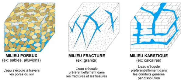
La présence de grands hydrosystèmes souterrains concernent une grande partie des sous-sols français (Figure 1.1). Ces aquifères sont globalement catégorisés en trois grands types structurels (Heath 1998) : les milieux poreux dans des sols non consolidés ou des roches poreuses, les milieux fracturés dans des roches consolidées ayant subi une fracturation et les milieux karstiques dans des roches carbonatées ayant subi une dissolution par action d’eau acide (Figure 1.2).

Ces trois types d’aquifères sont caractérisés par différentes structures géologiques qui génèrent des écoulements de plutôt diffus et lents au travers des pores en milieu poreux, à plutôt rapides et préférentiellement localisés dans les conduits en milieu karstique. De part ces différences de fonctionnements hydrauliques et hydrologiques, les études des aquifères requièrent de bien intégrer également leurs particularités morphologiques.

Figure 1.1: Gauche : Répartition des grands hydrosystèmes souterrains français (BRGM 2015). Droite : Répartition des formations karstifiables en France (Marsaud 1996).

Figure 1.2: Schématisation des écoulements dans trois types de milieux pouvant être aquifère : milieux poreux, fracturés et karstiques (modifié d’après Heath 1998).

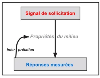
L’étude du fonctionnement hydrodynamique d’un aquifère repose sur la caractérisation de ses propriétés hydrauliques telles que la conductivité hydraulique et le coefficient d’emmagasinement. Ces propriétés contrôlent les modalités de transferts hydriques et des contaminants. Du fait de l’impossibilité de pouvoir accéder directement aux propriétés du milieu aquifère, excepté par des analyses d’échantillons de roches issus de forages qui ne fournissent que des informations locales, il convient d’estimer indirectement ces propriétés. Il est ainsi possible de les estimer, à partir d’investigations in situ, en interprétant les réponses d’un aquifère à divers types de sollicitations (pompage, injection traçage,…), puisque ces réponses dépendent de ces propriétés hydrodynamiques et reflètent leur hétérogénéité dans le milieu (Figure 1.3).

Figure 1.3: Schéma de la caractérisation des propriétés par interprétation des réponses à un signal de sollicitation.

Le choix du signal de sollicitation utilisé, de la quantité et de la répartition de réponses mesurées, et de la méthode d’interprétation de ces dernières sont autant de variables qui permettent d’adapter la caractérisation au type de milieu investigué et au type d’information qui est recherché (Butler 2005). Les types de sollicitation et de réponses mesurées sont liés par leurs interactions via les propriétés du sol. Il est ainsi possible d’investiguer un aquifère par pompage dans la nappe et de mesurer les réponses de rabattements (Figure 1.4) afin d’en estimer les conductivités hydrauliques.

Les approches d’investigation sont nombreuses et en constante évolution. Les méthodes « classiques » d’investigation d’aquifère sont présentées dans le Tableau 1.1.

Signal de sollicitation

Réponses mesurées

Propriétés du milieu

Figure 1.4: Représentation schématisée d’une investigation par pompage avec débit à signal constant d’un aquifère fracturé et karstique (modifié d’après Goldscheider et Drew 2007).

Tableau 1.1: Méthodes « classiques » d’investigation (Butler 2005 ; Bechtel et al. 2007 ; Hartmann et al. 2014). Le tableau présente le type de sollicitation et les réponses communément associées, ainsi que l’information qui peut en être retirée.

Sollicitation Réponses mesurées Informations interprétables

Pompage débit

constant Rabattement

Conductivités hydrauliques moyennées du volume impacté

Slug test Rabattement Conductivités hydrauliques locales autour du

forage

Traçage Concentrations Connectivités et vitesses d’écoulements

Pluie Variations de charges,

débit, concentrations

Réactivité physico-chimique du système, types d’écoulements

Courant électrique Différence de potentiel Résistivités, saturation des matériaux

Onde sismique Vitesse d’onde Structures géologiques sous-terraines

Champ gravimétrique

Micro-variation du

champ gravitationnel Localisation de vides

Electromagnétisme – Radar pénétrant

Variation de champ

magnétique Identification d’anomalies dans le sol

Potentiel spontané Potentiel électrique Identification et localisations des mouvements d’eaux

Il existe différentes méthodes pour interpréter quantitativement les propriétés d’un aquifère à partir des réponses mesurées. Globalement ces méthodes peuvent être classées en deux grandes catégories : les solutions analytiques et les solutions numériques. Les solutions analytiques sont basées sur des expressions mathématiques sous forme analytique, c’est-à-dire construites à partir des opérations arithmétiques basiques, qui se prêtent aisément au calcul. Ces solutions analytiques excluent néanmoins le caractère hétérogène des propriétés hydrauliques. Les solutions numériques, au contraire, permettent de pouvoir modéliser les réponses à des équations plus complexes par des méthodes de résolution des opérations différentielles (parmi lesquelles la méthode de différence finie, volume fini ou encore élément fini) en prenant en compte la variabilité spatiale des propriétés hydrodynamiques. Ainsi, un modèle distribué, basé sur une solution numérique, permet de simuler spatialement les réponses d’un aquifère à partir d’un champ de propriétés, en discrétisant et résolvant les équations d’écoulements sur un maillage. L’interprétation des réponses mesurées sur le terrain consiste dans ce cas à retrouver un champ de propriétés qui serait capable de reproduire, par simulation dans le modèle, les données de terrain.

La caractérisation numérique distribuée des aquifères s’est orientée vers des techniques de tomographies hydrauliques (Carrera et Neuman 1986b ; De Marsily et al. 1995 ; Yeh et Liu

2000 ; Delay et al. 2007). A l’instar des tomographies utilisées dans le domaine médical, elles

permettent d’imager, en plan ou en volume, les propriétés d’un milieu à partir de mesures ponctuelles de surface. La tomographie hydraulique repose d’abord sur la définition d’un problème direct, décrivant les lois associées aux phénomènes physiques qui sont employées pour la résolution du modèle. Puis, le problème inverse, basé sur le problème direct, optimise le champ de propriétés du modèle afin de reproduire les réponses mesurées lors de l’investigation. Schématiquement, le problème direct définit le lien entre les réponses au signal de sollicitation, alors que le problème inverse permet de reconstruire les propriétés du milieu dans le modèle, correspondant à l’interprétation des réponses recherchées (Figure 1.5). La tomographie hydraulique repose également sur la qualité et la quantité des données (réponses de l’aquifère), qui doivent permettre de bien caractériser le champ de propriété généré par le problème inverse (Yeh et Lee 2007). Si ces conditions sont réunies, la tomographie hydraulique peut alors être vue comme un outil d’imagerie des aquifères, qui peut ensuite servir l’interprétation et la discussion scientifique.

Figure 1.5: Schéma de la reconstitution des propriétés à partir d’un modèle direct et de l’inversion des réponses mesurées.

L’inversion est un processus mathématique, stochastique ou déterministe, qui aboutit à une ou des solutions possibles de champs de propriétés minimisant l’écart entre les données simulées et observées (Tarantola et Valette 1982). Le processus d’inversion stochastique consiste à générer itérativement un grand nombre de modèles de propriétés différents et d’en garder au final les meilleurs, qui approchent des solutions globales au problème (en s’appuyant sur la loi des grands nombres). Le processus déterministe se base plutôt sur une optimisation itérative d’un modèle initial, basée sur une étude de sensibilité, et convergeant au final vers un modèle de propriétés approchant une solution locale au problème (dépendante du modèle initial).

Néanmoins, dans les deux cas, ce processus purement mathématique est mal posé, avec une solution qui n’est pas unique, et peut donc aboutir à des résultats reproduisant les données de terrain, mais irréalistes physiquement ou structurellement. Il devient intéressant de pouvoir contraindre l’inversion à partir des connaissances a priori sur les propriétés du milieu, afin de limiter ses résultats à des solutions réalistes vis-à-vis du milieu. Ainsi de nombreux travaux ont visé à développer des manières de contraindre l’inversion, dont quelques-unes sont présentées dans le Tableau 1.2. Signal de sollicitation Réponses simulées Propriétés du modèle Inter prétation Problème direct Problème inverse Minimisation des écarts entre réponses mesurées et simulées

Tableau 1.2: Exemples de contraintes pouvant être appliquées sur des inversions afin de produire des distributions de propriétés adaptées aux connaissances des milieux.

Type de contrainte

Type de variation de distribution de

propriétés

Exemple de référence

Géostatistique Lisse Geostatistical approach (Hoeksema et Kitanidis

1984) Mathématique (loi

de distribution) Hétérogène Total variation prior (Lee et Kitanidis 2013) Structuration du

modèle direct Structurée Level set (Lu et Robinson 2006)

Guidage par image Structurée Training image (Lochbühler et al. 2015)

Image guided (Soueid Ahmed et al. 2015) Processus

physique Structurée Karstic network formation (Jaquet et al. 2004)

Résolution du champ de propriétés

Hétérogène Multi-scale (Grimstadt et al. 2003)

Les contraintes dans l’inversion visent à orienter les solutions vers une certaine forme de distribution spatiale des propriétés. Les solutions proposant des distributions trop éloignées des règles établies par les contraintes, sont écartées. Les contraintes peuvent être vues, schématiquement, à un contrepoids informatif à la reproduction purement mathématique des réponses, tel que représenté en Figure 1.6.

Figure 1.6: Schéma entre la liberté attribuée dans la reconstitution des réponses dans le processus d’inversion par rapport aux contraintes établies sur les solutions.

Les aquifères fracturés et karstiques génèrent des écoulements suivant des chemins préférentiels : via le réseau de fissures et fractures de la roche dans le premier cas, et via le réseau de conduits formés par dissolution de la matrice calcaire dans le second cas. Ces aquifères requièrent donc une attention toute particulière lors de l’investigation et dans l’interprétation numérique afin de caractériser le haut degré de contraste spatial existant dans leurs propriétés hydrodynamiques et qui provoque ces écoulements préférentiels.

De nombreux travaux de caractérisation d’écoulements se sont déjà intéressés à imager ces contrastes dans des modèles équivalents milieux poreux (Larocque et al. 1999 ; Abusaada

et Sauter 2013 ; Saller et al. 2013 ; Wang et al. 2016), dans des modèles à double continuum (Zimmerman et al. 2013 ; Kordilla et al. 2012), ou dans des modèles couplés discret-continu (Kovacs 2003 ; Jaquet et al. 2004 ; Saller et al. 2013). Des exemples de ces modèles sont

présentés en Figure 1.7.

Figure 1.7: Haut : Schéma des différentes techniques de modélisation distribuées issu de Ghasemizadeh et al. 2012 (EPM = Equivalent Milieu Poreux ; DPM = Milieu Double Porosité ; DFN = Réseau de Fractures Discrètes ; DCN = Réseau de Conduits Discrets ; HM = Modèle Hybride). Bas : Exemples de modélisations d’aquifères karstiques par (a) EPM (Saller et al. 2013), (b) DPM (Kordilla et al. 2012), et (c) HM (Kovacs 2003).

Néanmoins, il apparaît que la caractérisation spatiale des propriétés des milieux fracturés et karstiques requiert toujours le développement de nouvelles méthodes d’investigation et de modélisation qui permettront de mieux caractériser leurs écoulements très

contraints et d’apporter, pour ces milieux, des outils d’imagerie hydraulique pour une meilleure compréhension de leurs fonctionnements hydrodynamiques.

Les travaux menés dans le cadre de cette thèse visent à répondre à ce verrou en proposant de nouvelles approches tomographiques de caractérisation adaptées aux aquifères fracturés et karstiques.

Ces approches tomographiques reposent, d’une part, sur l’acquisition de données lors d’une phase d’investigation basée sur une méthode particulière de sollicitation de la nappe, par pompage harmonique, et de traitement et d’analyse des réponses oscillatoires du niveau hydraulique. L’utilisation de pompages harmoniques pour la caractérisation des milieux fracturés a été récemment étudiée par Renner et Messar 2006 et Guiltinan et Becker 2015. Leurs résultats montrent que cette technique d’investigation peut également être prometteuse pour les milieux karstiques, pour lesquelles elle n’a pas encore été particulièrement étudiée.

Ces approches tomographiques sont basées, d’autre part, sur une interprétation quantitative en utilisant des concepts de modélisation numérique des écoulements souterrains (type équivalent milieu poreux ou couplé discret continu) et de nouvelles méthodes d’inversions adaptées afin de représenter plus fidèlement les contrastes existant dans ces milieux en déterminant l’architecture spatiale des conduits karstiques.

Tout au long du manuscrit les résultats produits par applications de ces différentes nouvelles approches servent à alimenter une discussion sur les écoulements et échanges existant dans les aquifères fracturés et karstiques à l’échelle décamétrique.

Ce manuscrit est construit autour de six articles produits au cours de cette thèse :

· Chapitre 2 : Application of large-scale inversion algorithms to hydraulic tomography in an alluvial aquifer, Groundwater, 2017.

· Chapitre 3 : A cellular automata-based deterministic inversion algorithm for the characterization of linear structural heterogeneities, Water Resources Research, 2017.