Acoustic Boiling Detection
byGeorge Daniel Doney
B.S. Systems Engineering US Naval Academy 1992 B.S. Economics US Naval Academy 1992
Submitted to the Department of Nuclear
Engineering in Partial Fulfillmentof the Requirements for the Degree of
Master of Science
at theMassachusetts Institute of Technology
February 1994
r LUEj
C)
Massachusetts Institute of Technology 1994
All its
reserv
Signature of Author
Deartment of Nuclear Engineering
(7~
~
February
28,1994
Certified by/1
-U
'i/I z,Professor John E. Meyer
Thesis Supervisor
Certified by)
Professor David D. Lanning
Thesis Reader Approved by->
Professor Allan F. Henry
* r
cli
Acoustic Boiling Detection
by
G. Daniel Doney
Submitted to the Department of Nuclear Engineering
on February 28, 1994 in partial fulfillment of therequirements for the Degree of Master of Science
in Nuclear Engineering
Abstract
Experiments were performed to gather data on the effects of changing bulk
temperature and power levels on the sound of boiling. This information was formatted and
used to train a neural network to recognize boiling. The trained network was then used in
an executable program to provide an indication of boiling.
The trained network is an detector predictor of boiling under the experimental
conditions. More work must be done before the detector can be reliably used in the
reactor. With more development, the detector could possibly be used to provide important
coolant information for Pressurized or Boiling Water Reactors.
Thesis Supervisor:
Dr. John E. Meyer
Title: Professor of Nuclear Engineering Thesis Reader: Dr. David D. Lanning
Acknowledgments
I would like to extend a special thanks to the following people who contributed much of their time to help me with my thesis:
Professor William Clement: Professor Clement spent a lot of his time helping me to learn C this past summer. His ideas helped shape my work into its current format. He helped debug my programs and allowed me to use the neural network program he had written, DTRC93. He also helped me get the hardware used in the experiment.
Professor John Meyer: Professor Meyer was instrumental in helping me to express my ideas. He helped me change my thesis from a garbled mass to somewhat refined project (in a very short time). He also helped me to develop some of the ideas used in the detector. Professor David Lanning: Professor Lanning kept me funded for my stay here at MIT. Without money, I couldn't have done anything. He also helped me to revise my thesis. Professor Martin Nelson: Professor Nelson was very enthusiastic and helpful in offering his facilities at the Naval Academy for my summer work. It was there that I did my first work with highly subcooled boiling (and destroyed my first heater).
Robert Catalano and Benthos, Inc: Robert sent two free hydrophones to be used with
my experiment. These hydrophones served their purpose extremely well by providing excellent frequency resolution (the best things in life are free).Hernan Trosman: Hernan helped me to revise my thesis at the end when things became
hectic. I'm hoping he'll learn to use Borland C++ so he can advise whoever may come
along next to take up the project. He also ran to get me a 9V battery (even though I didn't
need it).Table of Contents
Abstract
...
Acknowledgments
...
Introduction
...
Chapter 1: Boiling
...
1.1 The Ideal Bubble ...
1.2 Boiling Types ...
1.3 Experimental Results ...
1.4 Subcooled Boiling Stages ...
Chapter 2: Background Noise
2.1 Duration ...
2.1.1 Transients ...
2.1.2 Persistent Noise.
2.2 Bandwidth ...
Chapter 3: Signal Analysis
...
3.1 Filters and Windows ...
3.2 Fourier Transform.
3.3 Logarithmic Scale ...
3.4 Normalization.
3.5 Neural Network ...
3.5.1 Reasons For Use ...
3.5.2 Training Procedure ...
3.5.3 Boiling Training ...
3.5.4 Non-Boiling Training ...
Chapter 4: The Boiling Detector
...
4.1 Definitions ...
4.2 Implementation ...
4.3 New Ideas ...
3
4
9
15
16 17 23 26 31 32 33 35 3841
41 42 43 44 46 48 50 51 5255
55 58 59...
...
...
...
...
...
...
...
...
...
...
...
...
...
...
...
...
...
...
...
...
...
...
...
...
...
...
...
...
...
...
...
...
...
...
...
...
...
...
...
...
Table of Contents
4.3.4 Fluctuations in the Power Spectrum
4.3.5 Power and Temperature Prediction
4.3.6 "Smart" Implementation ...
Conclusion
...
Appendix A: Experimental Hardware
A.1 Hydrophone
A.2 The Heating Element ...
A.3 Data Acquisition Board ...
A.4 CPU ...
Appendix B: User's manuals ....
B.1 Sampler ...
B.2 Filechan ...
B.3 DTRC94 ...
B.4 Boildet.exe ...
B.5 Fileread ...
References
...
... 6 3 . .. . . 6 3 . . . 6 4...
67
...
69
.. . ... . ... .. . .. . ... . .. .. . . .. .. . .. . . 6 9 .. . . ... ... . .. .. . . ... .. . . .. .. . . .. . . . 7 3 . . .. .. ... .. . ... . . . .. .. .. . .. .. .. . .. . 7 5 . . .. . .... .. .. .. . . .. . . . . .. .. . .. ... . . 7 6...
77
... 8 0.... ...
...
8 4
... 8 9 ... ... 9 8 ... 10 4...
107
6 .. . . .....
....
....
.......
List of Figures
Figure 1.1: Methanol Boiling Curve
...
15
Figure 1.2: Pressure Pulse of Bubble in Subcooled Liquid .. 20
Figure 1.3: Spectral Density of Pressure Pulse in
. 21
Subcooled and Saturated Liquid
...
Figure 1.4 Boiling at 46 deg C, 500 kW/m
2, no flow (1) and
. 25
-1
m/sec flow (2)
...
Figure 1.5 Boiling at 57 deg C, 200 kW/m
2, no flow
...
26
Figure 1.6: Boiling at 53 deg C, 500 kW/m
2, no flow
...
28
Figure 1.7: Boiling at 36 deg C, 700 (1) and 900 (2) kW/m
2,
. 29
no flow
...
Figure 2.1 Infinite Moving Average for Background
...
36
Figure 2.2 Diagram of Weighted Rolling Average
...
37
Figure 2.3 Narrowband and Broadband Noise Examples ....
39
Figure 3.1 Diagram of Neural Network
...
46
Figure 4.1: Diagram of Boiling Detector
...
55
Figure 4.2 Diagram of Path of Data
...
56
Figure A.1: Diagram of Experimental Setup
...
69
Figure A.2: Diagram of Hydrophone
...
71
Figure A.3: Possible Hydrophone Location
...
72
List of Figures
Figure B.1.1 Sampler Main Screen ...
78
Figure B.1.2 Create Boiling Screen ...
79
Figure B.2.1: Filechan Main Screen ...
82
Figure B.2.2: Filechan Edit Screen ...
83
Figure B.3.1 DTRC94 Main Screen
...
87
Figure B.3.2 DTRC94 Edit NetworkScreen
...
88
Figure B.4.1 Boiling Detector Main Screen
...
91
Figure
B.4.2
Change
Axis
Screen
...
92
Figure B.4.3 Boiling Detector Options Screen
...
93
Figure B.4.4 Edit Filters Screen
...
94
Figure B.4.5 Edit Equalizer Screen
...
95
Figure
B.4.6
Change Gain Screen
...
96
Figure B.4.7 Change Buffer Size Screen ...
97
Figure B.5.1: Fileread Main Screen
...
102
Figure B.5.2: Fileread Edit Structure Screen
...
103
Introduction
In the next few years, MIT may need to relicense its nuclear research reactor. In order to meet the research needs of the institution into the 21 st century, several proposals have been presented which allow the reactor to achieve higher neutron flux. One such proposal is to modify current MITR-II core and raise its power to 10MW. Studies are currently underway to determine if the current core can handle this higher power level. It may be possible, by increasing the flow rate and by reducing uncertainties associated with
the current safety system, to allow safe operation of the reactor at higher power with few
alterations to the current core.
Reactor limitations are set not just by the physical properties of the reactor but
also by the detectability of the conditions in the reactor. If a variable must be estimated through calculations, there will be uncertainties. In order to assure safety, operating limits
must be set to take into account the most conservative estimation of the variable. In a
system with a number of uncertainties, the limitation may be set far below the physical
limitation of the system in order to assure safety. This is the case with the high
temperature scram signals of the reactor. Thermocouples located in the reactor hot leg
piping are used to determine the average exit temperature of the coolant that leaves the
reactor. If the temperature, e.g. 60 degrees C, indicated in the Technical Specifications
has been exceeded a scram signal is produced since under certain core circumstances thisis an indication that the reactor is approaching a damaging operating condition. Damage to
the core is imminent if initiation of boiling causes a flow instability to occur in a channel. Athe fixed reactor parameters such as coolant channel thickness with variables such as flow rate, power density, coolant temperature, and pressure is used to determine the onset of flow instability. The expected coolant temperature at the outlet of the channel in which the flow instability may occur can then be determined as a function of channel power by
setting the pressure constant (pool type reactor) and using a minimum acceptable core flow rate (1800 gpm). If the maximum acceptable outlet temperature is known, the outlet temperature of the other channels can be determined if the flux distribution is known
throughout the core. The temperature of the mixed fluid can be compared to the measured
average exit temperature detected in the hot leg piping. This process may produce a scram signal. The temperature for safe operation is set much lower than the physical limitations due to uncertainty in channel conditions (flow rates, cladding thickness, etc. caused by manufacturing errors and changing conditions in the core), disparity between channels
(nonuniform flux distribution), uncertainty of data (errors or lack of coverage in
instrumentation), and variable recognition time (transport time of coolant).
The onset of flow instability for the MITR core is preceded by boiling in the
channel. Therefore, if an occurrence of boiling can be accurately detected soon enough,
the reactor can be safely shut down. This is a better method for preventing flow instability
than temperature detection, since the boiling information is explicit. For water cooled
reactors, when under-cooling conditions occur, boiling precedes dangerous reactor
conditions, however, under certain conditions (such as channel blockage) the bulk coolant
temperature may not exceed specifications while damage to the core is occurring.The uncertainty with a boiling detection system is whether or not the onset of
boiling is accurately established. With an accurate boiling detection system, therefore, the power can be raised much closer to the physical limitations, allowing better performance and more adequate safety. The engineering challenge is to produce an accurate boiling detector. It must not give false alarms which result in costly shutdowns and it must not miss a boiling occurrence that results in damage to the core.
Many methods have been developed to detect boiling but are not applicable for detection of boiling in the core, however. The method must:
1. detect boiling at any location in the core; 2. work in the harsh environment of the reactor; 3. fit in the limited space of the core;
4. not interfere with the operation of the reactor; and 5. be a financially attractive option.
For example, one method of boiling detection would be to measure temperature
fluctuations in the cladding temperature. But, boiling can occur at any point along the core axially or radially, so thermocouples would have to be placed at many points in the core,thus interfering with the operation of the reactor.
Another possibility is neutron flux noise detection. When boiling occurs in the
reactor, voiding in the moderator/coolant causes fluctuations in the neutron population in
the core. These fluctuations can be used to indicate boiling. Neutron noise boilingdetection requires accurate measurement of these fluctuations. Additionally these
fluctuations must be measured by multiple detectors axially to verify that the fluctuationsAcoustic boiling detection meets all of the conditions listed. Since sound travels through the coolant, an acoustic boiling detector would be able to detect boiling at any location. With the proper hydrophone, the detector can work in high flux and high temperature conditions. The hydrophone can be placed in a location so it can be easily replaced in the event that its performance becomes degraded. The hydrophone is small so
it does not interfere with reactor operations. Since it does not need to be located in the
core, it is not difficult to find a location in the hot or cold leg for it. The detector system is inexpensive since the only hardware is a hydrophone, a data acquisition board, and a
computer (the costs of these items are listed in Appendix A).
Acoustic boiling detection is not a new idea. Experiments to measure the acoustic
noise have been done on sodium for liquid metal cooled reactors', methanol2, and water
cooled reactors
3with the possibility for use for detection in mind. This paper furthers the
research done in the area of boiling detection by developing new techniques for
measurement and attempting to apply these techniques to provide a working detector. The
method for separating the signal of interest has been improved and a neural network was used to analyze boiling signal. These improvements allow detection and analysis at varying
levels of background noise characteristic of nuclear reactors over a range of pressures,
Srinivasan,G.S.and O.P Singh, "New Statistical Features Sensitive to Sodium Boiling Noise", Ann. Nucl. Energy, Vol. 17, No. 3, pp. 135-138, 1990.
2 Westwater, J.W, A.J. Lowery, Jr., and F.S. Pramuk, "Sound of Boiling", Science,
Vol 122, 332-333, 1955.
Koski, J.A., A.G. Beattie, J.B. Whitley, and C.D. Croessmann, "Experimental
Verification of Subcooled Flow Boiling for Tokamak Pump Limiter Designs", The
American Society of Mechanical Engineers papers, 345 E. 47 St., New York, N.Y. 10017, 1987.
temperatures, flow rates, and power levels. Potentially, the detector may allow the operator to determine these parameters at the point where boiling is occurring.
14
Chapter 1: Boiling
In order to anticipate the signal received under different conditions in the core, knowledge of the origin and sound of boiling is required. Initially, subcooled boiling aids the ability to carry away energy from the surface. But as power is increased in a low pressure, plate type reactor, boiling leads to flow instability which may reduce the energy removal capability of the coolant.
There are a number of boiling regimes described in two phase flow books. Two of
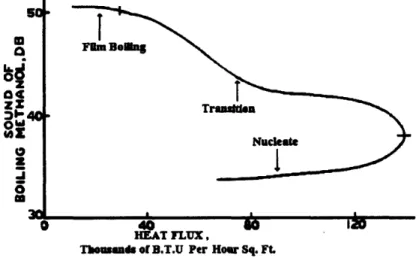
these regimes, nucleate boiling and film boiling were studied in other investigations to determine the heat transfer characteristics and noise magnitude. One study used methanol as the coolant and produced curves which related the degree of subcooling, the heat flux, and the overall magnitude of the boiling noise (Figure 1.1).
o50 U
a
z
04
zz
36 40 ow0
z -Ia
w MC 0 40 s0 IZo HEAT FLUX,Tboumkad of B.T.U Per Hour Sq. Ft.
Figure 1.1: Methanol Boiling Curve4
The results show that during nucleate boiling, the amount of heat removed 0.
in heat flux only results in small increases in boiling noise. But at a certain point, the boiling regime undergoes a transition to film boiling. At this transition point (indicated by a dash in Figure 1.1), the boiling noise increases dramatically and the heat removal capabilities of the heater are reduced. This causes the temperature to continue to go up and causes a further reduction of the ability of the coolant to remove the heat. At this point, if power is not reduced, damage to the heating element is likely. In the present
study, experiments involving film boiling were not made in order to avoid damage to the heating element.
In this chapter, different types of nucleate boiling will be investigated to give a
better idea of what to look for when attempting to detect boiling.
1.1 The Ideal Bubble
Boiling is a thermodynamic process in which vapor is produced to form a bubble in the surrounding liquid. In the process of expanding and contracting, the bubble gives off pressure pulses (sound) which travel through the water. An object immersed in water which expands and contracts emits in the far field a pressure wave, P.:
I!
Pac
=v
Paci r V Eqn. 1.15
where:
p=
density of the liquid;
V'=
second time derivative of the emitting body volume evaluated at time t-r/c with
c= speed of sound in media; andr= distance from source
5 Nesis, Y. I., "Acoustic Noise of a Boiling Liquid", Heat Transfer - Soviet
Research, Vol. 22, No. 6, 1990. Translated from Two-Phase Flow: Heat Transfer and Unsteady-State Processes in Turbomachinery. USSR Acad. Sci., pp. 68-74.
Therefore the creation and collapse of vapor bubbles will create an associated
pressure pulse which can be picked up as sound.
If all other parameters are kept constant, as the power introduced to the liquid is
raised, distinct changes in the type of bubble formed will occur, causing changes in thesound associated with boiling. Understanding these changes is important for detection of
boiling.
1.2 Boiling Types
Three types of boiling are listed in a paper entitled "Acoustic Noise of a Boiling Liquid"6. First, vapor oscillation which occurs as microscopic gas bubbles perform free radially-symmetric pulsations with a cyclic frequency in the bulk of the fluid is discussed.
These oscillations create very low magnitude pressure pulses and are not important to this
analysis.
As the amount of the heat transfer to the liquid is increased, the near wall layer
adjacent to the heating surface will experience a sharper temperature gradient. If the temperature gradient is large enough the liquid at the wall surface will reach saturation temperature. This situation results in subcooled boiling since the bulk temperature is still
below saturation.
Bergles-Rohsenow Eqn:7
2.3
/,
qONB
=
15.6
p
1 5 6[ATsAT
I
]
0234Eqn 1.2
where:qoNB (BTU/hr m2)= Heat flux necessary for onset of nucleate boiling (ONB); P (psi)= pressure at the boiling site; and
ATS
T(deg F)-
TWAL-TAT..
Notice that the greater the degree of bulk liquid subcooling, the more heat flux is
required to cause boiling. Therefore, as the bulk temperature increases, less power is
needed to cause boiling.
The rest of Chapter 1.1 is a summary of information presented in "Acoustic Noise
of a Boiling Liquid"
8The equations listed are taken from this paper.
Subcooled boiling is characterized by rapid growth and separation of small vapor bubbles that exist at the heat source. As these bubbles depart from the heating surface,
first they increase in size due to the evaporation of superheated or saturated liquid near
wall layers. At some point, the bubble will come in contact with cooler liquid and the expansion will stop with the bubble reaching some maximum radius, R. The bubble will
then collapse as its energy is absorbed into the surrounding liquid. The time that the
bubble takes to reach cooler water will decrease if the temperature gradient is higher. The
Todreas, N.E., Kazimi M.S. Nuclear Systems I. Hemisphere Publishing
Corporation, 1990, page 534, Eq. 12.16
8 Nesis, ibid.
temperature gradient, remember, is a function of the subcooling, AT,, = T,,t-Tb,. The bubble lifetime, o, is inversely proportional to its maximum size, Rm.
k
To
=
k
Eqn 1.3
0
ATsub
-Rm = k2
*
ATSub
Eqn 1.4
The field generated by a multitude of such bubbles is the sound of subcooled boiling. The bubbles may vary slightly in size, but there will be a mean size, the variation
about which depends on the uniformity of the boundary layer. In order to determine the
frequency spectrum of subcooled boiling, the spectrum created by a single bubble of mean size will be investigated. Assuming that the bubbles are spherical in shape, the bubble volume as a function of radius (R) can be inserted into Equation 1.1 yielding:
Pac
=PR[2(R
)
2+(R*R)]
Eqn
1.5
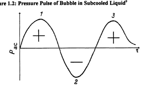
Analysis of this equation gives an idea of the acoustic pulse associated with the ideal
bubble (Figure 1.2). With subcooled boiling, the radius of the bubble increases from 0 to
Rm, then decreases again to 0. At small values of R, the first term in brackets on the RHS
of Equation 1.5 is obviously greater than the second term. Therefore, early in the life of the bubble, while it is small but growing, a compression pulse will be emitted (Condition
(Condition 2). As the bubble begins to collapse, the collapse decelerates causing another compression pulse (Condition 3). This conclusion matches the experimental measurements of a single bubble in a subcooled liquid.
Figure 1.2: Pressure Pulse of Bubble in Subcooled Liquid9
U
r0
Changing the conditions, under which boiling occurs will change the magnitude
and may alter the period of the pressure pulse, but the pulse will not change qualitatively.
The spectral density S(o) of the pulse can be found by taking the Fourier integral:
oo
S(o)= IPac(t)@eidt
--00
Eqn 1.6
The frequency (co) of maximum amplitude, IS(O)I,j, produced by the a subcooled bubble with the P,(t) shown in Figure 1.2 is:
9 Nesis, ibid.
20
(Ormx- 3x
0Eqn 1.7
since there are 3 sign changes in the pulse.
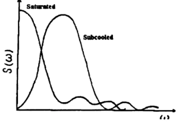
The sound which results from a multitude of bubbles (see Figure 1.3) with a maximum radius,
Ra,
which is distributed about a radius, Rmmea, can be easily verifiedsince the spectrum of the sum of the signals is equal to the sum of the spectra of each
signal taken separately.Under conditions of subcooled boiling there is no strict repetition of pressure
pulses emitted by bubbles. Therefore, the resulting spectrum is continuous with a broad maximum. Also, equidistant narrow maxima can be isolated that correspond to the periodic repetition of the origination and collapse of bubbles (see Figure 1.3).
Figure 1.3: Spectral Density of Pressure Pulse in Subcooled and Saturated Liquid
-C
3e
If the bulk temperature of the fluid is at saturation, a third type of bubble will be formed. This bubble is characterized by its large size. An investigation of the pressure
larger. After a time, a temperature decrease at the interface with the liquid becomes
noticeable and the rate of growth decreases:
R(tt
Substituting R(t) into Equation 1.5 results in a pressure pulse tapering to zero. But, since the bubble never collapses, there is no rarefaction pulse. Notice that a major portion of the frequency spectrum associated with boiling is in the infrasonic range (frequency below zero) (see Figure 1.3), and therefore cannot be heard.
Subcooled boiling noise is the best indicator of trouble necessitating shutdown.
The temperature of the coolant in the MIT reactor is such that saturated boiling is not
likely to occur. Other methods of shutdown, such as temperature detection prevent bulk
temperatures from getting to this point. Also, since subcooled boiling will likely precede boiling which causes instability in the channel, detection of subcooled boiling is enough. Detecting saturated boiling alone does not exclude the possibility of damage to a fuel element since damage to an element can occur without the bulk temperature ever reaching saturation. Therefore, it is clear that detection of subcooled boiling is the case of interest in the present study.
Fortunately, subcooled boiling is both a better indicator of trouble and easiest to
detect (not only because it is louder, but also because its characteristic frequencies areabove the range of most commonly occurring background noises). Low frequencies, like
those in which saturated boiling occurs, are cluttered with background noise.
1.3 Experimental Results
The data gathered in the experiments of the present study can be analyzed with the background information from the previous section. Altering the conditions in which boiling occurs changes the characteristics of the bubble which in turn affects the sound of boiling. Understanding the differences is essential for detection in the reactor since the detector may be required to identify boiling under any of these conditions.
Experiments were performed using the setup shown in Figure A.1. For a detailed
description of the hardware see Appendix A. First, the heater was turned on to a low
power setting (50 kW/m2) and background samples were taken. This provides a better background frequency spectrum (see Chapter 3.2 FFT) since there is noise while the heater is running even if no boiling was occurring. The background spectrum consists of the average of 50 spectra taken at low power. The background was updated periodicallythroughout the experiment to account for changes.
The power was then increased and spectra were taken in bursts periodically. Each
recorded spectrum is actually the average of 50 spectra minus the background spectrum.
5-20 spectra were recorded in each burst.
When each burst was taken, a value was assigned to each spectrum in the burst to
tell whether and what type of boiling was occurring. These values could be changed later on further inspection. Also the bulk temperature of the fluid, measured approximately 15 cm from the heater, was taken in order to demonstrate the effects of changing temperature
the heater was shaken in a wide path. The estimated velocity of the heater was 1 m/sec. Also, all frequencies below 0.5 kHz were clipped in each of the plots shown. Frequencies lower than this are dominated by background noise like amplifier bias and flow noise. The frequency domain of the voltages produced by the amplifier are plotted. The relative amplitude between plots is partially dependent on the amplifier gain which may change from day to day. Any plots with more than one spectrum were taken at nearly the same time so the amplifier gain will not be a factor.
An increase in the subcooling decreases the lifetime of the bubble (Equation 1.3). The more violent growth and collapse results in a louder peak sound which is centered about a higher frequency. Also, there is less variation in the bubble lifetimes, since the boundary layer is thinner, resulting in a more defined frequency peak.
Increasing the pressure also affects the vapor bubble. A higher pressure with a
given bulk temperature increases the amount of subcooling. Also, the thermodynamic equilibrium is changed resulting in a bubble which is differently shaped giving a different frequency spectrum. Studies must be done at high pressures to determine the exact
correlation between the frequency spectrum and the pressure.
Impurities in the coolant will have a slight effect on the frequency spectrum. As
dissolved non-volatiles come out of solution, they provide a means for vapor bubbles to
form. These bubbles are short lived (except the non-volatile part) and may skew thespectrum slighly towards higher frequencies. Impurities affect the saturation temperature
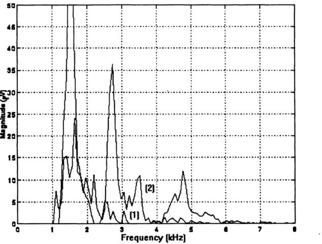
as well and increase the degree of subcooling.The coolant flow rate past the heated surface also affects the frequency spectrum. Turbulent flow reduces the boundary layer at the surface of the heater. This means the bubbles will be short lived. Therefore, the bubbles grow and collapse with tremendous ferocity resulting in a very loud peak which can be over 10 times louder than the no flow peak (Figure 1.4). Since the boundary layer is thin, the bubble lifetime is fairly uniform so the peak is very narrow. Interestingly, the center frequency of the peak is very close to the center frequency under no flow conditions (with the same liquid subcooling and
pressure).
Figure 1.4 Boiling at 46 deg C, 500 kW/m2, no flow (1) and -1 m/sec flow (2) __
a
a
Il
1.4 Subcooled Boiling Stages
Subcooled boiling has been observed to occur in several distinct stages as the heat flux is increased. The onset of nucleate boiling (ONB) occurs after the wall temperature
has exceeded the saturation temperature by some amount. This stage of subcooled boiling
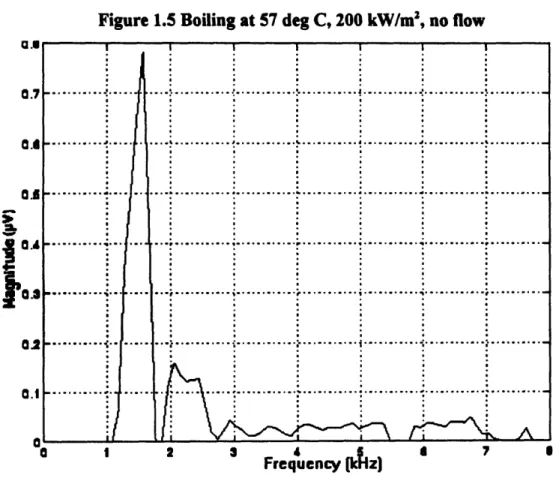
is marked by a single frequency peak as mentioned in Chapter 2.1.2. Many observationswere taken of boiling near its onset. One example of an observed spectrum, Figure 1.5, is
very similar to the multiple ideal bubble spectrum shown in Figure 1.3..
With the heater at constant power and the temperature nearly constant
(observation taken over a period of a few seconds), the magnitude of the peak frequency
fluctuated. This is probably due to oscillations in natural circulation past the heated
surface. These oscillations had a period on the order of a second.Figure 1.5 Boiling at 57 deg C, 200 kW/m2, no flow
Frequency [kHzJ
26
Observations performed several minutes apart give an indication of the difference in the spectrum with changing degree of subcooling. As long as the boiling remained in the onset stage, there was little difference in the peak frequencies over the temperature range expected in the core.
However, the boiling noise appears to have gone through other stages. If the
power were increased at a constant temperature or if temperature increased at constant
power, at a certain threshold, the boiling frequency spectrum pattern would change. The
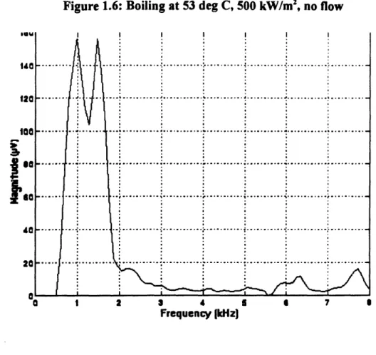
changes were not simply an increase in the magnitude of the peak or a shift in the peak frequency. The changes suggest different types of bubble being formed.The second stage (or regime) of subcooled boiling initiates when an additional frequency peak begins to grow (Figure 1.6). This additional peak is at a lower frequency
than the first. As power or temperature continue to rise this second peak grows in
magnitude to levels higher than the initial peak. Since the peaks are closely spaced, if
power continues to increase, the peaks become one.
Figure 1.6: Boiling at 53 deg C, 500 kW/m2, no flow
.QU
Frequency IkHz)
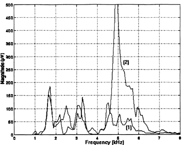
As power is raised even higher a third peak begins to grow (Figure 1.7). This
broad peak occurs at a much higher frequency than the other two. As power continues to
rise, the magnitude of this peak dominates the first two. Observations were not made at
power levels higher than this in order to avoid damage to the heater. Explanations for the
onset of these peaks is beyond the scope of my research but further analysis may lead to
interesting theories about the stages which occur before damage to a fuel element.
28
Figure 1.7: Boiling at 36 deg C, 700 (1) and 900 (2) kW/m
2, no flow
_z 0 1 2 3 4 1 a 7 IFrequency
[kHz)
5 S 4 3 Sar
:2 1 1 IChapter 2: Background Noise
Noise is any disturbance registered by the detector. Noise may affect the detector's ability to determine if boiling is occurring. These disturbances may lead to false alarms or prevent detection. Of particular interest is background noise. Background is any signal which is not the signal of interest. Any measurement taken will always have background. If there is too much background noise, the detector may be incapable of making a reliable estimation of the conditions. Eliminating or reducing noise is paramount to successful boiling detection. Therefore, understanding and predicting the background noise is the
topic of this chapter.
Background noise can come from many sources which can be electrical or acoustic. Electric disturbances or noise may result from faulty wiring or poor equipment. This creates a cost tradeoff since equipment which produces the least electrical noise is
often the most expensive. But if the electric noise is low relative to the amplitude of the
desired signal, the additional clarity afforded by more expensive equipment may not be worth the cost. Once information is digitized, it is not susceptible to more noise.Acoustic noises are the pressure disturbances received by the hydrophone which are then converted to an electric signal. The acoustic noise has a greater effect on the detection of boiling so it will be the focus of this section. Sources of acoustic noise include
the coolant pumps, movement of the control blades, the flow of water, and the creation
The sources of noise, whether electric or acoustic, can be broken down into
several categories. Background noise can be classified according to its duration and
bandwidth.
2.1 Duration
Background noise may persist or may be transient. Persistent background noise is a signal which lasts longer than an arbitrarily set period of time. This period of time
depends on the frequency of sampling and is relative to the components which make up
the signal. For example, if pump noise levels were being measured once a day, changes inthe level of noise which took hours to take place would produce fluctuations considered
transient. But if spectra were being updated every second, a change in the level which
took several hours to take place would appear persistent from one sample to the next.
Conditions in a nuclear reactor consist of transient and persistent components
regardless of the time scale chosen. For a boiling detector, the required time scale is
determined by the time in which shutdown must be initiated for safe shutdown after
boiling has occurred. The detector must have updated itself at least once within this
period. This requires updating spectra every fraction of a second. Background noise
whose level changes unappreciably over this time interval will be considered persistent. A pump in steady state operation or an electrical bias on an amplifier are examples of
persistent noise.
Transients are noise which occurs in a time period on the order of one sample
interval. The sound produced when dropping the control blades is an example. It is
interesting to note that pump noise may also be a transient during startup. Faulty connections also result in transient noise when the wires are bumped.
Attempts to reduce transient background noise are limited by the need for rapid detection of boiling. Attempts to eliminate persistent background noise are limited by the desire to avoid identifying slowly developing boiling as background noise. Each technique helps focus on boiling but does not eliminate all background noise from being presented to
the detector.
2.1.1 Transients
The primary method of reducing the relative magnitude of transients is to increase
the length of time of the buffer containing the data to be analyzed (sample time). The Fast
Fourier transform (FFT discussed in Chapter 3) produces a frequency spectrum which has
the average magnitude of the frequency component during the sample period. If the
sample time is longer than the existence of the transient, the average value of the transient
will be proportionally less. For example, if a 10 OV source were introduced for .1 second
and then stopped and the sample time were I second, the magnitude of the source would
appear to be V when averaged over the length of the entire signal.
Secondly, the larger the sample time the more computer memory is required to store and analyze the sample. For instance, at a sampling rate of 40 kHz, 320kBytes of
memory are required to store double precision data for a one second sample time. Since
high sampling rates are required in order to distinguish all frequencies in the boiling rangeorder of 25 milliseconds. This is not enough time to reduce all but the shortest transients, so more provisions are required to provide adequate reduction of transients.
In addition to increasing the sampling time, sequential samples can be averaged together. By increasing the number of samples averaged, short transients can be eliminated. Averaging forty 25 millisecond samples together will result in an effective sampling time of 1 second.
By requiring the detector to identify boiling on more than one consecutive
spectrum, false alarms caused by transients can be limited. This also limits carry-over between spectra averaged which can result in false alarms even for very short transients which are high in amplitude. But the user must be careful not to require too many consecutive boiling signals before the boiling alarm is set off, since the alarm may be unduly delayed.
The time required for initiation of shutdown of the reactor from the onset of
boiling limits the time period of each sample. Hypothetically, if a sample is analyzed for boiling every 10 seconds, transients which lasted only I seconds would be reduced 2
orders of magnitude. But if boiling began at one second, and if, again hypothetically, in
order for safe shutdown the reactor, scram must be initiated 4 seconds after the onset of
boiling, the signal would be received 5 seconds too late. Therefore the sampling periodmust be shorter than the difference between the time from the onset of boiling to the time
when scram is mandatory for safe shutdown. In fact it should be significantly shorter to allow for measurement error and additional safety margins.2.1.2 Persistent Noise
Any source which remains constant is not difficult to remove. If indeed the source
is constant, the background spectrum can be measured at one point in time then subtracted
from subsequent spectra. Unfortunately, no sound source in the reactor is completely constant. Each source will have small variations with time and must both start and stop atsome point. As a result, the background spectrum will change with time. Therefore, the
spectrum subtracted from subsequent spectra must be able to adapt to the changing
conditions in the core. Appropriate allowance for a moving background accomplishes this.In order to avoid confusion and simplify the discussion, I will name various spectra
used in the detection of boiling. The source spectrum is the spectrum entering the
computer, the background spectrum is the moving average, and the net spectrum is the
difference between the two.
When a source is received, it is subtracted from the moving background producing a net spectrum. The net spectrum is then analyzed to determine if boiling is occurring. The
source is then averaged with the background to produce a new background spectrum and
the procedure is repeated.
One problem with this method is the boiling will be quickly integrated into the
background. This means that just a few sampling periods after boiling has begun, the net
spectrum used to identify boiling will be close to zero even though boiling continues. Thiscould result in missed detection.
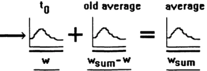
tO old average average
W Wsum-W Wsum
Figure 2.1 Infinite Moving Average for Background
The source and background spectra can be weighted to reduce this effect.
Decreasing the weight given to the source spectrum will decrease the rate at which a
steady state signal is incorporated into the background spectrum.
Consider, for example, a step signal introduced to a constant background. The
weights for this example are assigned such that the ratio (r) of the spectrum weight (w) to
the sum of the weights (w ) is 0.1. The first time step after the step signal has been
introduced the source spectrum will be the background plus the step spectrum. The
average will consist of 90% (l-r) of the background and 10% (r) of the source spectrum.
When this average is subtracted from the source spectrum, the result is the net spectrum.
The net spectrum will be 90% of the source spectrum. After the second time step with the
same source, the average will again consist of 90% of the old average and 10% of the
source, but remember the old average has 10% of the source. Therefore, the net spectrum
will be 81% (l-(r+r*(1-r))) of the source. If the source remains constant after this point,
the net spectum, s, after n time steps will be:
n
S= 1 r(l+ r
i
(1- r)
i=o
After 3 time steps, the step boiling will still have approximately 73% of its magnitude. If the signal introduced contained boiling, the detector would only see 73 percent of the magnitude of the spectrum. After a period of time, the net spectrum presented for analysis may be too small to be recognized.
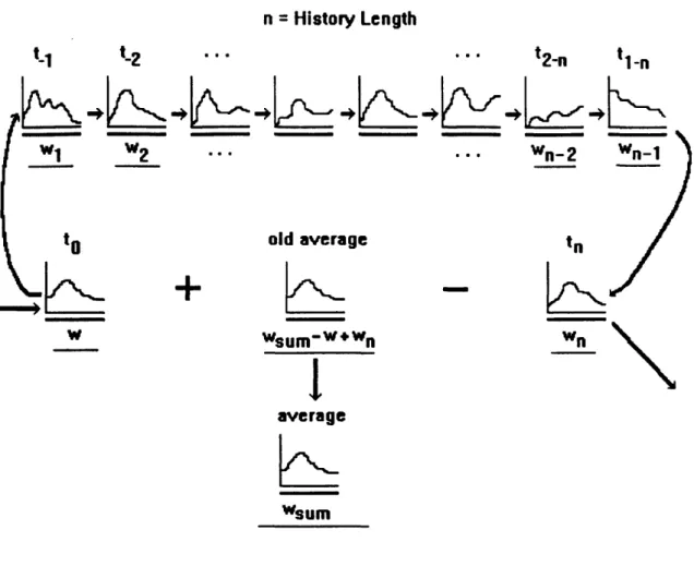
n = History Length
t-l
t-
2.·'..
t2.
ntl-n
4
-L:-t
4
+
Li2 L
4
LŽ
W2 ... Wn-2 old average tn+
I
I o
_-[
K w Wsum-w*wn wn average WsumFigure 2.2 Diagram of Weighted Rolling Average
With an infinite moving average (see Figure 2.1), a small part of every spectrum
problem, old spectra should be subtracted from the background, thereby alleviating their influence. This is called a rolling average (see Figure 2.2). In order to keep a rolling average, a history of the spectra must be kept (the longer the history the more memory is required). Old samples are stored to the disk along with their weights so they can be removed later. Since the disk will be accessed with each new spectrum introduced, the computer must be able to store and retrieve information from disk quickly.
Additionally the weight to assign a source can be determined by the output of the
detector. If the detector indicates boiling is occurring no weight is assigned to the
spectrum. This means than the spectrum will not be integrated into the background
spectrum and a boiling spectrum on the next sample will not have lost any intensity. If boiling occurs for an extended period of time, the weights assigned to all the spectra in the history could potentially become zero. This would mean the detector would "forget" what any of the background looked like. To solve this, if the weight is zero (i.e.
boiling is occurring), the spectrum is not written to the background history, after all it is
not background and if the sum of all the weights goes below some threshold, new spectra
are not written to the history unless their weight is higher (i.e. less representative of
boiling) than the spectrum they are replacing. This procedure is an excellent way of adapting to changing background signals without missing signals which are boiling.
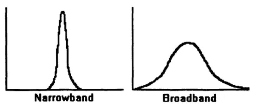
2.2 Bandwidth
Noise sources in the reactor will have different bandwidths. The energy from narrowband noise is concentrated about a few frequencies while broadband noise energy
extends over a wide range of frequencies. (see Figure 2.3). The exact cuttoffbetween
broad band and narrowband noise is relative. In this case, spectra with energy extending over a greater energy than a typical boiling spectrum are considered broadband
(aproximately an increment of .5 kHz).
Narrowband
Broadband
Figure 2.3 Narrowband and Broadband Noise Examples
Pump noise is an example of narrowband noise while turbulence in flowing water produces a broader frequency spectrum. By properly setting the frequency resolution, the influence of broadband or narrowband noise can be reduced. There are several tradeoffs which must be made in choosing a frequency resolution.
First, there is the tradeoff between reduction of broadband and reduction of
narrowband noise. Since the energy is spread out over a range of frequencies, increasing resolution makes broadband noise less significant. Conversely, since the energy is focused about one frequency, decreasing resolution makes narrowband noise less significant. Therefore the resolution should be close to the bandwidth of a boiling spectrum.
Reducing the frequency resolution decreases the pattern recognition abilities of the
detector. For example, if the boiling spectrum had two peaks which were very close in
frequencies characteristic of boiling fall into more than one frequency bin. This helps eliminate the possibility of mistaking boiling with a narrowband of another source.
As mentioned in Chapter 1, the frequencies characteristic of boiling change with changing conditions in the reactor. With a low resolution detector, small changes in the associated frequencies with changing conditions will not result in a change in the distribution in the frequency bins.
As the frequency resolution is increased additional computer processing time is
required. Depending on the speed of the computer running the detector, this can be a very
limiting factor. Additionally increased resolution results in increased demands on thecomputers memory. This has been perhaps the most limiting factor on this project.
Chapter 3: Signal Analysis
Processing the signal is a very important step in reliable boiling detection. Separating and identifying the signal of interest is challenging due to the changing
conditions in the core. This chapter describes the techniques used to remove extraneous
data as the information passes through the detector.
3.1
Filters and Windows
The signal from the amplifier can be sent through an analog filter before being received by the computer. A analog low pass filter should be used for anti-aliasing (see Chapter 3.2 FFT). A passive filter can be easily and cheaply implemented without requiring an external power source. This choice reduces the likelihood of system failure. The low pass filter should have a have a corner frequency at approximately 8 kHz which is above the upper frequency expected of boiling (see Figures 1.4 & 1.5). The filter is not essential to successful boiling detection since, in general, noise with frequencies above half the sampling rate are uncommon. However, the filter does not require CPU time and it is easy to implement and maintain.
After being filtered, the signal is sent to an analog to digital (A/D) converter where
the analog voltage is converted to digital value between of 0 and 2047. This information is put into a buffer where it can be downloaded to computer memory. The total time span of each buffer is the sampling rate, f,, multiplied by the number of samples, k. After downloading to computer memory, the samples can then be digitally filtered.
information available. The choice of a window is application specific. A Blackman window was chosen for this application since it provides excellent frequency resolution.
The signal can then be sent through any of a variety of digital filters. One
possibility is to send the signal through a digital equalizer. The frequency range of interest can then be emphasized. The most important frequencies are in the range of 1 to 3 kHz
but other important boiling frequencies occur in the 3 kHz to 8 kHz range.
Signals below 500 Hz are also characteristic of boiling but are frequently masked by random background noise in this range. Therefore, this information is not useful for boiling detection. This range can be filtered out or simply not analyzed.
3.2 Fourier Transform
The signal is still in the time domain. It would be difficult to extract patterns from time domain data when a number of frequencies are involved. Differences in phase make even a simple single frequency wave look radically different to the neural network making
training difficult to impossible. By performing a Fourier transform on the data, the signal
can be converted to time averaged amplitudes in the frequency domain. The magnitude of
the resulting complex spectral data is called the power spectrum. Since the power
spectrum contains no phase dependence, it is easier to analyze.
In order to take a Fast Fourier Transform, the number of samples in the buffer
holding the data must be a power of two. The formula for the Fast Fourier transform isl:
42
10 Lab Windows Advanced Analysis Library Reference Manual, Vol 2.3. National instruments, 1993.
k-1
Y [co]
=
X[t *
e
xp(-iot
, for o= 0, l *fop /k, 2*f,/k,..., (k-)*f,p k
t=0The result of the Fast Fourier Transform is k discrete frequency bins of complex data. The k-length array of the magnitude of each frequency bin is the power spectrum. As
mentioned earlier, the size of the buffer, k, also determines the frequency resolution. The transformed data is aliased which means that the spectrum is mirrored about half the sampling frequency. Aliasing is a result of discrete data. Therefore, the sampling
rate of the A/D converter must be set to at least twice the highest expected frequency of
boiling (see Figure 1.4 & 1.5). Only the lower half of this data is of interest to boiling
detection. Therefore, the size of the buffer containing the spectrum to be analyzed is k/2.
After the background has been subtracted from the source, the resulting spectrum
is clipped. Any values which are below zero are unimportant for analysis since boilingdoes not absorb sound.
3.3 Logarithmic Scale
Some time was spent determining if the logarithmic scale should be used to modify
the data before being sent to the network. The advantage of the logarithmic scale is that
data the several orders of magnitude difference can be analyzed. The logarithmic scalewould be beneficial for use with the detector if the boiling (or important characteristics of
orders of magnitude smaller at 4 kHz, the second peak would be lost without the logarithmic scale. This could cause a failure to recognize the type of boiling occurring.
The net spectrum may be zero if, for example, a noise source in the background has been shut off and the background spectrum has not had time to adjust. The logarithm of zero is negative infinity which would throw off detection. Therefore a threshold must be
set. Values less than the threshold are set equal to the threshold and then evaluated.
Although the logarithmic scale may be shown to be an improvement with fUrther investigation, it is not essential for boiling detection. Any frequencies characteristic of
boiling seem to give peaks of the same order of magnitude. Without the logarithmic scale,
the peaks associated with boiling stand out since they are several orders of magnitude
above the random background noise. This makes boiling easily detectable.3.4 Normalization
The spectra are normalized with the maximum magnitude of the power spectrum
being set to 1 and everything else being scaled. There are several advantages to
normalized spectra. First, the distance and the number of obstructions between the actual
boiling event and the hydrophone cannot be known. Therefore, boiling occurring under
precisely the same conditions but at different locations would have different magnitudes. It
is important that the computer recognize the spectral pattern associated with boiling not
characteristic magnitudes. The detected patterns seem to be independent of the type of
boiling or even whether or not boiling is occurring. Additionally, this means the network can be trained with the hydrophone one distance from the boiling and implemented a44
different distance away. Since testing in the core is unlikely until the final stages of development, this will enable the network to be trained in lab conditions.
In addition to different detector locations affecting the magnitude of the spectrum, the conditions in which boiling is occurring affect its magnitude as well as the frequency distribution. The spectra are more uniform and easier to recognize when normalized. This prevents missed signals at low or high extremes of boiling.
Normalizing the spectrum does have its disadvantages. First, if a noise significantly louder than boiling occurs at a different frequency while boiling is occurring, the boiling may be overwhelmed. Therefore, the spectrum should be normalized about the range in which boiling is expected and values above this range should be clipped.
Also, the magnitude of the spectrum contains important information about the
boiling. For a binary boiling detector, where the operator is only concerned whether or not
boiling is occurring this information is not important. But for a detector which makes anestimation of the power level, flow rate, and pressure, where the boiling is occurring, the
magnitude of the spectrum is important information. Therefore, the normalizing value can
be included as an input to the detector.
A random fluctuation may also be mistaken for boiling if the spectrum is
normalized. To prevent this a threshold should be set. A spectrum whose maximum value
is below the threshold should not be entered in the network for consideration as boiling.
3.5 Neural Network
OUTPUTS
Output Layer (5 Neurons)
Hidden Layer 2 5 Neurons)
Hidden Layer (5 Neurons)
Input Layer [100 Neurons]
bias
Figure 3.1 Diagram of Neural Network
Neural networks offer a means by which the computer can "learn" to recognize and classif y information. They are modeled after the human brain. The advantages of
neural networks make them excellent tools for many scientific applications. Further
explanation on the theory and implementation of neural networks can be found in Neural
Computing". A summary on the theory and application of neural networks was taken from
this text.
In an artificial neural network, the unit analogous to the biological neuron is referred to as a "processing" element. A processing element "PE" has many input paths (dendrites) and combines, usually by a simple summation, the values of these input paths. The result is an internal activity level for the PE. The combined is then modified by a transfer function. This transfer function can be a threshold function which only passes information if the combined activity level reaches a certain level, or it can be a continuous function of the of the combined input. The output value of the transfer function is generally passed directly to the output path of the processing element.
Neural Computing, NeuralWare, Inc. 1991. pp. NC3-NC7.
The neural network used by the boiling detector uses a sigmoid function with a straight line above a certain threshold.
The output path of a processing element can be connected to input paths of other processing elements through connection weights which correspond to the synaptic strength of neural connections. Since each corresponding connection has a corresponding weight, the signals on the input lines to a processing element are modified by these weights prior to being summed.
Thus the summation function is a weighted summation. In itself, this simplified model of a neuron is not very interesting; the interesting results come from the way neurons are interconnected. A neural network consists of many processing elements joined together in the above manner.
Processing elements are usually organized into groups called layers. A typical network consists of a sequence of layers with full or random connections between layers. There are typically two layers with connections to the outside world: An input buffer where data is presented to the network, and an output buffer which holds the response of the network to a given input.
The network used for the boiling detector has an input layer with 100 neurons, an
output layer with 5 neurons, and two hidden layers of neurons with 5 neurons each.(seeFigure 3.2)
There are two distinct phases in the operation of a network - Learning and Recall. In most networks [including the one used by the detector] these phases are distinct. Learning is the process of adapting or modifying the connection weights in response to stimuli being presented at the input buffer and optionally at the output buffer. A stimulus presented at the output buffer corresponds to a desired response to a given input; this desired response must be provided by a knowledgeable teacher. In such a case the learning is referred to as "supervised learning."
In the case of the boiling detector, the information provided to the input buffer is
the normalized frequency spectrum. The output of the detector is the type of boiling
(which is represented by four binary numbers) and potentially the conditions of boiling (i.e.Another type of learning is unsupervised learning which may not be applicable to the boiling detector. A third type of learning called reinforcement learning has the network learn by having the user indicate whether its output is "bad" or "good". This type of network should receive further investigation but was not applied to the current detector.
Whatever kind of learning is used an essential characteristic of any network is its learning rule which specifies how weights adapt in response to a learning example. Learning may require showing the network many examples thousands of times. The parameters governing a learning rule may change over time as the network progresses in its learning. The long term control of the learning parameters is referred to as its learning schedule.
The learning schedule was particularly important for the training of the network. If
too many boiling spectra or non-boiling spectra were given in a row, the network learned
down the wrong path and oscillated, unable to get over a threshold.
The recall stage is done at run time and refers to the way in which the network
responds to various stimuli. At this point, the network does not continue to learn. If in the
future, the operator decides that the network is not functioning adequately, it will have to
be retrained.3.5.1
Reasons For Use
The use of the neural network has many advantages over other methods of
detection for this particular application. Boiling detection is a pattern recognition
procedure, in which the incoming pattern may change with a variety of background
conditions and changing boiling parameters. One advantage of the neural network is faulttolerance.
48
Whereas traditional computing systems are rendered useless by even a small amount of damage to memory, neural computing systems are fault tolerant. Fault tolerance refers to the fact that in most neural networks, if some processing elements are destroyed, impaired, or disabled, or
their connections altered slightly, then the behavior of the network as a whole is only slightly degraded. As yet more processing elements are destroyed, the behavior of the network is degraded just a bit further. Performance suffers, but the system does not come to an abrupt halt. Neural
computing systems are fault tolerant because information is not contained in one place, but is distributed throughout the system. This characteristic of fault tolerance or graceful degradation makes neural computing systems extremely well suited for applications where failure of control equipment means disaster: In nuclear power plant operation, missile guidance, space probe operation, and so on.
The boiling detector is an application which requires robust detection. Since the
input to the detector is the power spectrum of the signal from the hydrophone, the
spectrum will be complete, but it may be cluttered with background noise and it is possible
that part of the boiling spectrum may be drowned out by a loud background noise.
Neural computing systems are adept at many pattern recognition tasks, more so than both traditional statistical and expert systems. The human ability to translate the symbols on this page into meaningful words and ideas is a form of pattern recognition. Pattern recognition tasks require the ability to match large amounts of input information simultaneously and then generate
categorically generalized output. They also require a reasonable response to noisy or incomplete input. Neural computing systems possess these capabilities as well as the ability to build unique structures specific to a particular problem, so they are particularly useful in pattern recognition. The ability to select combinations of features pertinent to the problem gives them an edge over statistically based systems. The ability to deduce features on their own is an advantage over expert systems used in pattern classification.
Boiling noise comes in the form of distinct patterns. The overall magnitude is not
as important as the particular spectrum shape for an indication of boiling. The shape
changes depending on the conditions which eliminates the applicability of many statistical
methods.
3.5.2 Training Procedure
To train the network, the spectra are taken and formatted in the same manner that
they would be for use with the detector. The spectra are identified manually when taken.
The boiling spectra are separated into different regimes* and the non-boiling spectra are
identified.If the spectra are grouped together according to their type, the network may learn
down one path for one type of boiling and then follow a separate path for non-boiling,
causing it to oscillate about the right answer. To prevent this, the order of the spectra
must be randomized before feeding to the information to the neural network.
*regime refers to a group of spectra with similar frequency spectra which are likely representative of a particular type of boiling