HAL Id: hal-02559412
https://hal.archives-ouvertes.fr/hal-02559412
Submitted on 30 Oct 2020
HAL is a multi-disciplinary open access
archive for the deposit and dissemination of
sci-entific research documents, whether they are
pub-lished or not. The documents may come from
teaching and research institutions in France or
abroad, or from public or private research centers.
L’archive ouverte pluridisciplinaire HAL, est
destinée au dépôt et à la diffusion de documents
scientifiques de niveau recherche, publiés ou non,
émanant des établissements d’enseignement et de
recherche français ou étrangers, des laboratoires
publics ou privés.
communities in the Guaymas Basin
M. Portail, K. Olu, E. Escobar-Briones, J. C. Caprais, L. Menot, Matthieu
Waeles, P. Cruaud, P. M. Sarradin, A. Godfroy, J. Sarrazin
To cite this version:
M. Portail, K. Olu, E. Escobar-Briones, J. C. Caprais, L. Menot, et al.. Comparative study of vent and
seep macrofaunal communities in the Guaymas Basin. Biogeosciences, European Geosciences Union,
2015, 12 (18), pp.5455-5479. �10.5194/bg-12-5455-2015�. �hal-02559412�
www.biogeosciences.net/12/5455/2015/ doi:10.5194/bg-12-5455-2015
© Author(s) 2015. CC Attribution 3.0 License.
Comparative study of vent and seep macrofaunal communities
in the Guaymas Basin
M. Portail1, K. Olu1, E. Escobar-Briones2, J. C. Caprais1, L. Menot1, M. Waeles3, P. Cruaud4, P. M. Sarradin1, A. Godfroy4, and J. Sarrazin1
1Institut Carnot Ifremer EDROME, Centre de Bretagne, REM/EEP, Laboratoire Environnement Profond,
29280 Plouzané, France
2Universidad Nacional Autónoma de México, Instituto de Ciencias del Mar y Limnología, AP 70-305,
Ciudad Universitaria, 04510 México, D. F.
3Université de Bretagne Occidentale, IUEM, Lemar UMR CNRS 6539, 29280 Plouzané, France
4Laboratoire de Microbiologie des Environnements Extrêmes, UMR6197, IFREMER, UBO, CNRS, Technopôle Brest Iroise,
29280 Plouzané, France
Correspondence to: M. Portail (marie.portail@ifremer.fr)
Received: 10 April 2015 – Published in Biogeosciences Discuss.: 10 June 2015 Accepted: 10 August 2015 – Published: 21 September 2015
Abstract. Understanding the ecological processes and
con-nectivity of chemosynthetic deep-sea ecosystems requires comparative studies. In the Guaymas Basin (Gulf of Cali-fornia, Mexico), the presence of seeps and vents in the ab-sence of a biogeographic barrier, and comparable sedimen-tary settings and depths offers a unique opportunity to as-sess the role of ecosystem-specific environmental conditions on macrofaunal communities. Six seep and four vent as-semblages were studied, three of which were characterised by common major foundation taxa: vesicomyid bivalves, si-boglinid tubeworms and microbial mats. Macrofaunal com-munity structure at the family level showed that density, di-versity and composition patterns were primarily shaped by seep- and vent-common abiotic factors including methane and hydrogen sulfide concentrations, whereas vent environ-mental specificities (higher temperature, higher metal con-centrations and lower pH) were not significant. The type of substratum and the heterogeneity provided by foundation species were identified as additional structuring factors and their roles were found to vary according to fluid regimes. At the family level, seep and vent similarity reached at least 58 %. All vent families were found at seeps and each seep-specific family displayed low relative abundances (< 5 %). Moreover, 85 % of the identified species among dominant families were shared between seep and vent ecosystems. This
study provides further support to the hypothesis of continuity among deep-sea seep and vent ecosystems.
1 Introduction
Cold-seep ecosystems are related to active and passive mar-gins and along-transform faults, whereas hydrothermal vents occur along mid-ocean ridge systems, back-arc basins and off-axis submarine volcanoes. According to their geologi-cal contexts, these ecosystems involve distinct geochemigeologi-cal processes that give rise to fluid emissions from beneath the seafloor. At seeps, high pore-water pressures within sedi-ments result in the ascent of interstitial fluids that are en-riched in hydrocarbons (e.g. methane). As these fluids reach the upper sediment layers, methane is partly oxidised by mi-crobial consortia coupling an anaerobic oxidation of methane (AOM) with sulfate reduction that produces hydrogen sul-fides (Boetius et al., 2000). In contrast, at vents, seawater penetrates the ocean crust fissures and heats up until advec-tion processes initiate the rise of hot fluids (up to 400◦C) on the seafloor. The fluid composition becomes highly complex in contact with subsurface rocks, with enriched concentra-tions in trace, minor and major elements, methane, hydro-gen sulfide, hydrohydro-gen gas and dissolved metals (Von Damm, 1995; Jannasch and Mottl, 1985). Although seeps and vents
belong to two different geological contexts, both ecosys-tems are characterised by fluid emissions that present unusual properties, such as the presence of high concentrations of toxic compounds, steep physicochemical gradients and sig-nificant temporal variation at small spatial scales (Tunnicliffe et al., 2003). Furthermore, they both generate energy-rich flu-ids that sustain high local microbial chemosynthetic produc-tion in deep-sea ecosystems, which are usually food-limited (Smith et al., 2008). There, bacteria and archaea rely mainly on the oxidation of methane and hydrogen sulfide, which are the two most common reduced compounds in vents and seeps (McCollom and Shock, 1997; Dubilier et al., 2008; Fisher, 1990).
As a result, these chemosynthetic ecosystems share many ecological homologies. They harbour macrofaunal commu-nities that are heterogeneously distributed in a mosaic of dense assemblages defined by the presence of foundation species. These foundation species include dense microbial mats dominated by Beggiatoa, siboglinid polychaetes, vesi-comyid and bathymodiolid bivalves, alvinellid tube-dwelling worms, and several gastropod families (Govenar, 2010). Globally, vent and seep communities share elevated faunal densities, a relatively low taxonomic diversity and a high level of endemism in comparison to non-chemosynthetic deep-sea ecosystems (Tunnicliffe and Fowler, 1996; Sibuet and Olu, 1998; Carney, 1994). Vent and seep communities also share some families and genera, presenting evolutionary connections via common ancestors, with many transitions between vent and seep habitats over geological time (Tun-nicliffe et al., 1998; Tyler et al., 2002). Growing evidence of evolutionary and functional homologies rapidly highlighted potential links between the two ecosystems. Further support for this hypothesis was provided by the presence of species shared between seeps and vents and by the discovery of addi-tional chemosynthetic stepping-stones such as large organic falls (Smith and Baco, 2003; Smith and Kukert, 1989). More-over, macrofaunal communities at a recently discovered hy-brid seep and vent ecosystem called a “hydrothermal seep”, associated with a subducting seamount on the convergent Costa Rica margin, harbours both seep and vent features, thus providing additional support for the hypothesis of continuity among reducing ecosystems (Levin et al., 2012).
Despite these numerous homologies, comparison of seeps and vents at the macrofaunal community level have revealed striking differences. Comparative studies have shown that seeps exhibit usually higher diversity and lower endemism than vents (Sibuet and Olu, 1998; Turnipseed et al., 2003, 2004; Levin, 2005; Bernardino et al., 2012). Furthermore, the number of species shared on a global scale between the two ecosystems is less than 10 % of the total recorded species (e.g. Tunnicliffe et al., 2003, 1998; Sibuet and Olu, 1998). In addition, a recent review of several sedimented sites in the Pacific Ocean also points to strong dissimilarities between vent and seep macrofaunal communities even at the fam-ily level (up to 93 %; Bernardino et al., 2012). These strong
differences are assumed to be partly shaped by large-scale factors. Seep and vent biogeographic isolation and subse-quent evolutionary divergence, as well as the closer prox-imity of seeps to continents (and the resulting settlement of background macrofauna) may play an important role in structuring these communities (Carney, 1994; Baker et al., 2010). Nevertheless, around Japan, a region where a total of 42 seep and vent ecosystems are found in close prox-imity, the similarity between seep and vent species reached only 28 % (Watanabe et al., 2010; Sibuet and Olu, 1998; Nakajima et al., 2014). Therefore, other factors may con-tribute to the strong differences among communities. De-spite strong variation in environmental conditions in each type of ecosystem, due to the multiplicity of geological con-texts and environmental settings in which seep and vent oc-cur, vents are usually considered as less favourable to life than seeps. Vent fluids usually exhibit greater temperature anomalies, higher metal concentrations, lower pH and oxy-gen concentrations, as well as higher outflow rates and tem-poral instability, than seep fluids (Tunnicliffe et al., 2003; Sibuet and Olu, 1998; Herzig and Hannington, 2000). There-fore, ecological processes driving community dynamics and regulating community structure may indeed differ in seeps and vents. Although reliance on chemosynthetic production and tolerance to environmental conditions underlie the pre-dominant role of fluid input in both ecosystems, additional vent-specific factors may lead to distinct community struc-ture patterns among ecosystems and thus explain, at least partly, the seep and vent faunal discrepancies. Nonetheless, the effect of vent-specific environmental factors on the struc-ture of macrofaunal communities are not well known due to strong correlations among physicochemical factors (Johnson et al., 1988), preventing estimation of their respective effects (Govenar, 2010; Sarrazin et al., 1999). Overall, the key ques-tions that remain to be addressed involve the relative influ-ences of biogeographical and environmental barriers on vent and seep macrofaunal community dissimilarities (Bernardino et al., 2012).
The Guaymas Basin is one of the only areas in the world that harbours both ecosystems in close proximity. Located in the central portion of the Gulf of California, Mexico, the Guaymas Basin is a young spreading centre where hydrother-mal vents are found at less than 60 km from cold seeps with-out a biogeographic barrier, at comparable depths (around 2000 m) and in a similar sedimentary setting (Simoneit et al., 1990; Lonsdale et al., 1980). Therefore, this study site offers a unique opportunity to assess and compare the role of local seep and vent environmental factors on macrofaunal commu-nities.
Here, we compared the structure (abundance, diversity and composition) of Guaymas seep and vent macrofaunal assem-blages in relation to their environmental conditions. The fol-lowing questions were addressed: (1) what are the similari-ties and differences in geochemistry, microbial processes and potential engineering effects of foundation species within
and between ecosystems? (2) Does the structure of seep and vent macrofaunal communities differ and which abiotic and biotic factors can best explain community structure patterns? (3) What is the level of macrofaunal overlap between the two ecosystems and how does it relate to environmental condi-tions?
We tested whether macrofaunal density, diversity and composition patterns are ecosystem-dependent. We assumed that macrofaunal composition overlap among seeps and vents will be larger among low flux than among high fluid-flux sites. Finally, we hypothesised that other factors such as the nature of the substratum and the engineering role of foundation species may further add a non-negligible hetero-geneity within both ecosystems.
2 Materials and methods 2.1 Study area
This study focused on three areas in the Guaymas Basin located in the central portion of the Gulf of Califor-nia (Fig. 1): (1) cold seeps on the Sonora margin trans-form faults (27◦360N, 111◦290W) at 1550 m depth, (2) a large hydrothermal field on the Southern Trough depres-sion (27◦000N, 111◦240W) at 1900 m depth and (3) an off-axis reference site (27◦250N, 111◦300W) located at 1500 m depth.
The Guaymas Basin, due to the high biological pro-ductivity of surface water, is lined with a 1–2 km layer of organic-rich, diatomaceous sediments (Schrader, 1982; Calvert, 1966).
The Sonora margin transform faults are located along the eroding crest of a steep anticline (Simoneit et al., 1990; Paull et al., 2007). They are structurally similar to continental shelf pockmarks and have been named hydrocarbon seeps due to the emission of methane and higher hydrocarbon compo-nents. The fluid geochemistry is still poorly known (Simoneit et al., 1990). Extensive carbonate concretions have been re-ported and studied in this area (Paull et al., 2007). Macrofau-nal communities of the Sonora seep are mostly unknown and only foundation species (vesicomyid bivalves and siboglinid tubeworms) have been described (Simoneit et al., 1990; Paull et al., 2007).
The Southern Trough spreading segment is characterised by magmatic intrusions that drive an upward hydrother-mal flux through the organic-rich overlying sediments and maintain a recharging seawater circulation (Gieskes et al., 1982; Lonsdale and Becker, 1985; Fisher and Becker, 1991). End-member fluid composition is enriched in hydrogen sulfide, low-molecular-weight organic acids, petroleum-like aliphatic and aromatic hydrocarbons, ammonia, and methane (Kawka and Simoneit, 1987, 1990; Simoneit et al., 1996; Leif and Simoneit, 1995), but has relatively low metal con-centrations (Von Damm et al., 1985). Vent fluids emanate
ei-ther diffusely through the water–sediment interface at tem-peratures less than 200◦C or through mounds and chimneys rising over the seafloor where temperatures can reach up 350◦C (Von Damm et al., 1985). The foundation species of this vent area have been described (Soto and Grassle, 1988; Ruelas-Inzunza et al., 2003, 2005; Lonsdale and Becker, 1985; Demina et al., 2009), but only few studies have in-cluded the associated macrofaunal community (Grassle et al., 1985; Soto, 2009; Blake and Hilbig, 1990).
The Biodiversity and Interactions in the Guaymas Basin (BIG) cruise was held in 2010 on board the oceano-graphic vessel R/V L’Atalante equipped with the Nautile submersible. The autonomous underwater vehicle (AUV) AsterX explorations of the area resulted in the fine-scale mapping of active seep and vent sites (Fig. 1). In the vent field, we studied two hard substrate edifices, Rebecca’s Roots and Mat Mound as well as two sedimented vents, Mega Mat and the newly discovered Morelos site. At the seep, all study sites were newly discovered. Juarez site was characterised by carbonate concretions overlying soft sediments whereas Vasconcelos and Ayala were related to soft-sediment sites. All study sites are found deeper than the main oxygen min-imum zone (< 0.5 mL L−1) that is found between 650 and 1100 m along the north-east Pacific margins from the state of California to Oregon (Helly and Levin, 2004) and within the Guaymas Basin (Campbell and Gieskes, 1984). Oxygen measurements made in overlaying waters at our seep and vent study sites showed oxygen concentrations of 1.38 and 1.43 mL L−1, respectively.
2.2 Sampling design
The Nautile submersible was used to identify and sample specific assemblages, characterised by the presence of foun-dation species, within seep and vent sites. An off-axis site was also sampled and used as a background reference site of the Guaymas Basin (G_Ref).
Sonora margin
A total of six seep assemblages were studied S_ (Fig. 2). Three assemblages were sampled at the Vasconcelos site: (1) S_Mat characterised by microbial mats dominated by the
Beggiatoa genus, (2) S_Gast characterised by Hyalogyrina
sp. gastropods forming grey mats surrounding the micro-bial mats, and (3) S_VesA characterised by the dominance of Archivesica gigas vesicomyids that were found at the pe-riphery of white and grey mats. At Ayala, another type of Vesicomyidae assemblage was sampled: (4) S_VesP charac-terised by the dominance of Phreagena soyoae (syn. kilmeri). Some specimens of Calyptogena pacifica vesicomyids were sampled in qualitative peripheral samples at S_VesA and S_VesP. Finally, at the Juarez site, two assemblages were sampled: (5) S_Sib characterised by the siboglinid tube-worms Escarpia spicata and Lamellibrachia barhami
estab-Figure 1. Localisation of the study sites on the Sonora margin cold seeps (Ayala, Vasconcelos and Juarez sites), the Southern Trough
hydrothermal vents (Rebecca’s Roots, Mat Mound, Morelos and Mega Mat sites) and the Guaymas Basin off-axis reference site.
lished on carbonate concretions and (6) S_Sib_P correspond-ing to the presence of reduced sediments in the immediate periphery of S_Sib.
Southern Trough
A total of four vent assemblages were studied V_ (Fig. 2). At the Mega Mat site, a microbial mat assemblage was sampled: (1) V_Mat, characterised by the presence of white Beggiatoa sp. microbial mats surrounded by yellow Beggiatoa sp. mats. At the Morelos site, a Vesicomyidae assemblage was sam-pled: (2) V_VesA characterised by A. gigas vesicomyid. At the Rebecca’s Roots site, an alvinellid assemblage was sam-pled on the 13 m edifice: (3) V_Alv characterised by the presence of Paralvinella grasslei and P. bactericola. Finally, at the Mat Mound site, a siboglinid assemblage on a 3–4 m high sulfide mound was sampled: (4) V_Sib characterised by
Riftia pachyptila embedded in microbial mats.
2.3 Characterisation of physicochemical conditions
To characterise the habitats of the different assemblages, all sampling and measurements were performed in close prox-imity to the organisms (Table 1). Habitat temperatures were recorded using the Nautile temperature probe. Water sam-ples were collected in Fenwal Transfer Pack™ containers (2 L, Baxter) using the PEPITO sampler implemented on the Nautile submersible. The samples were pumped with a titanium–Tygon inlet associated with the Nautile temperature probe. Immediately after submersible recovery, the
contain-ers were brought to a clean laboratory and filtered through 0.45 µm Millipore® HATF filters for further quantification of dissolved metals (Fe, Mn and Cu). Fe and Mn were de-termined using inductively coupled plasma-optical emission spectrometry (ICP-OES; Ultima 2, Horiba Jobin Yvon, Pôle Spectrométrie Océan), whereas Cu was measured using a gold microwire electrode (Salaün and van den Berg, 2006). pH measurements (NBS scale) were performed on board us-ing a Metrohm glass electrode. Methane concentrations were quantified using the headspace technique (HSS 86.50, Dani-Instruments) and a gas chromatograph (Perichrom 2100, Al-pha MOS) equipped with a flame-ionisation detector (Sar-radin and Caprais, 1996).
For characterising soft-sediment habitats, we took addi-tional temperature measurements within the sediment layer, using a 50 cm long graduated temperature sensor as well as push-core samples. The pore waters were extracted from each 0–2 cm section along cores and analysed for methane, hydrogen sulfide, sulfate and ammonium concentrations fol-lowing procedures described in (Caprais et al., 2010; Vi-gneron et al., 2013; Russ et al., 2013). The CALMAR benthic chamber (Caprais et al., 2010) was used to characterise the methane flux at the interface of vesicomyid assemblages.
Data on physicochemical factors were analysed for all habitats when available and for soft-sediment habitats only. To compare all habitats, physicochemical factors from water measurements on hard substratum habitats were compared against physicochemical factors from sediment pore waters in soft-sediment habitats. For both types of substrata,
physic-Table 1. Abbreviations, sampling details and locations of the different assemblages sampled in the Guaymas Basin. Blade corers sample a
surface of 18 cm2for the small blade cores (SBC) and 360 cm2for the large cores (LBC), whereas tube corers (TC) sample a surface of 26 cm2. GS: ground surface sampled.
Abbreviation Latitude Longitude Foundation Substrata Physicochemical Faunal sampling
taxa characterisation
Reference assemblage
2 TC Macrofauna: 4 SBC
G_ref 27◦25.4830N 111◦30.0760W None Soft 5 PEPITO Microbiota: 1 TC
2 CALMAR Seep assemblages
1 TC Macrofauna: 3 LBC
S_VesP 27◦35.3650N 111◦28.3950W P. soyoae Soft 7 PEPITO Microbiota: 1 TC
2 CALMAR
1 TC Macrofauna: 3 LBC
S_VesA 27◦35.5870N 111◦28.9630W A. gigas Soft 2 CALMAR Microbiota: 1 TC
3 PEPITO
2 TC Macrofauna: 3 LBC
S_Mat 27◦35.5800N 111◦28.9860W Beggiatoa spp. Soft 12 PEPITO Microbiota: 1 TC
S_Gast 27◦35.5830N 111◦28.9820W Hyalogyrina sp Soft 2 TC Macrofauna: 1 SBC
Suction sampler +
S_Sib 27◦35.2740N 111◦28.4060W E. spicata, Hard 6 PEPITO submersible arm grab
L. barhami GS: 694 cm2
S_Sib_P 27◦35.2730N 111◦28.4070W None (S_Sib Soft 1 TC Macrofauna: 4 SBC
periphery) Microbiota: 1 TC
Vent assemblages
2 TC
V_VesA 27◦00.5470N 111◦24.4240W A. gigas Soft 8 PEPITO Macrofauna: 3 LBC
2 CALMAR Microbiota: 1 TC
V_Mat 27◦00.4450N 111◦24.5300W Beggiatoa spp. Soft 1 TC Macrofauna: 2 LBC
Microbiota: 1 TC
V_Alv 27◦00.6640N 111◦24.4120W P. grasslei, Hard 2 PEPITO Suction sampler
P. bactericola GS: 720 cm2
Suction sampler +
V_Sib 27◦00.3860N 111◦24.5760W R. pachyptila Hard 5 PEPITO submersible arm grab
GS: 1134 cm2
ochemical factors were separated into “interface” and “max-imum” concentrations, which represented fluid input prox-ies. On hard substrata, the interface values corresponded to the measurements made close to the substratum and max-imum values were selected from all measurements made within the three-dimensional assemblages. Similarly, soft-sediment physicochemical conditions from pore waters were summarised as interface values (0–2 cm) and maximum val-ues along the depth of the cores (10 cm).
2.4 Quantification of sedimentary microbial populations using quantitative PCR
At each location, a sediment push core was collected for mi-crobiological analyses (Table 1). After recovery on board, sediment cores were immediately transferred to a cold room (∼ 8◦C) for sub-sampling. Sediment cores (0–10 cm) were sub-sampled in 2 cm thick layers and then frozen at −80◦C for subsequent total nucleic acid extraction. For each sample, total nucleic acids were extracted using a method modified from (Zhou et al., 1996) and detailed in (Cruaud et al., 2014). Archaeal and bacterial abundances were then estimated by
Figure 2. Images of studied assemblages at seeps: (a)S_Mat and
S_Gast, (b) S_VesA, (c) S_VesP, (d) S_Sib and S_Sib_P and vents:
(e) V_Mat, (f) V_VesA, (g) V_Alv and (h) V_Sib.
quantitative polymerase chain reaction (qPCR). Amplifica-tions were performed with a Step One Plus instrument (Life Technologies, Gaithersburg, MD, USA) in a final volume of 25 µL using PerfeCTa® SYBR® Green SuperMix ROX (Quanta Bioscience), 1 ng of crude nucleic acid extract (tem-plate) and primers with appropriate concentrations accord-ing to the manufacturer’s instructions. The primers used tar-geted specific microbial groups potentially involved in AOM. Relative abundances of known clades of anaerobic methane-oxidisers (archaeal anaerobic methanotrophs ANME-1, -2 and -3; Vigneron et al., 2013) and their potential bacterial partners DSS (Desulfosarcina/Desulfococcus group), DBB (Desulfobulbus group) and SEEP-SRB2 (Vigneron et al., 2014) were estimated. Standard curves were obtained in trip-licate with 10-fold serial dilutions (105–109 copies per µL) of plasmids containing environmental 16S rRNA genes of selected microbial lineages. The efficiencies of the reactions were above 85 % and coefficients of determination (R2) of standard curves were close to 0.99. Samples were diluted
un-til the crossing point decreased log-linearly with sample dilu-tions, indicating the absence of an inhibition effect. qPCR re-sults were cumulated along the entire length of the sediment core and expressed in copy number per gram of sediment.
2.5 Macrofaunal community characterisation
For soft substrata, blade corers (180 or 360 cm2)were used to collect macrofauna (Table 1). On hard substrata, suction sam-pling before and after grab samsam-pling with the submersible arm was used to collect the macrofauna and samples were placed in individual isothermal boxes. Although quantitative sampling of soft-sediment communities is straightforward with box corers, it is much more difficult to carry out on hard substrata. Video imagery is therefore used to assess the pled surface. Numerical images taken before and after sam-pling were analysed using the Image J Software (see proto-col in Sarrazin et al., 1997). Each sampled area was outlined and analysed 5 times to estimate mean surface values. This method probably underestimates the sampled surfaces due to the omission of relief or thickness of the macrofaunal cover-age, inducing a bias in density estimates but no other method is yet available to quantitatively sample the macrofauna on hard substrata in the deep sea (Gauthier et al., 2010).
2.5.1 Foundation species
The distribution of foundation species was used a priori to define assemblages; we therefore excluded them from the community level study. Furthermore, these species can have both allogenic (e.g. bioturbation, sulfide pumping) and au-togenic (e.g. habitat provision) engineering effects on the structure of macrofaunal communities (Cordes et al., 2010; Govenar, 2010). For consistent approximation of potential engineering effects across assemblages, we used their size, biomass (ash-free dry weight (AFDW) without tubes for si-boglinids and without shells for vesicomyids and gastropods) and densities of foundation species as proxies.
2.5.2 Macrofaunal communities
All sediment sub-samples and hard substrata samples were sieved through a stack of four sieves of decreasing mesh sizes (1, 0.5, 0.3 and 0.25 mm). The samples were fixed in 4 % buffered formaldehyde for 24 h then preserved in 70 % al-cohol. In the laboratory, only macrofauna (> 250 µm) sensu stricto (i.e. excluding meiofaunal taxa; Hessler and Jumars, 1974; Dinet et al., 1985) were sorted, counted and identified. Identification was done to the lowest taxonomic level pos-sible with particular attention paid to dominant taxa. Poly-chaete morphological identifications at the species level were not systematically reached due to the sieving process which often damages the organisms. Bivalve identifications were made in collaboration with Elena Krylova (Shirshov Insti-tute of Oceanology, Russia), although a large number of juve-niles could not be identified to the species level. Gastropods
were exhaustively characterised in collaboration with Anders Warén (Swedish Museum of Natural History, Sweden). Be-cause it was not always possible to determine to the species level, comparisons of the macrofaunal community were done at the family level, except for some taxa with low con-tributions to macrofaunal densities, such as Aplacophora, Sipuncula, Scaphopoda, Nemertina, Cumacea, Tanaidacea and Amphipoda.
2.6 Data analyses
At the assemblage scale, considering the low level of repli-cation within some assemblages (n varied between 1 and 4, Table 1) and differences in sampling strategies between soft and hard substrata, data analyses mainly relied upon descrip-tive statistics. Rarefaction curves and Hurlbert’s ES(n) di-versity index were computed using the Biodidi-versity R pack-age (Kindt and Coe, 2005) and the functions in Gauthier et al. (2010) on pooled abundances per assemblage. The ES(n) measure of diversity was used because this index is the most suitable for non-standardised sample sizes (Soetaert and Heip, 1990). Spearman rank correlations were carried out on physicochemical variables, foundation species de-scriptors and associated macrofaunal community density and ES(n) diversity. Two levels of analysis were applied: one considering all assemblages sampled (hard and soft) and a subset focusing on soft-substratum assemblages, thereby al-lowing the addition of supplementary physicochemical vari-ables and the abundance of microbes potentially involved in AOM. Parametric regression models were tested for ES(n) and macrofaunal density in relation to physicochemical con-ditions to compare our data with previous studies.
Community composition analyses were based on Hellinger-transformed family densities to conserve Hellinger, rather than Euclidian, distances in the prin-cipal component analysis (PCA). The Hellinger distance gives a lower weight to dominant taxa and avoids consid-ering double absence as an indicator of similarity between samples (Legendre and Gallagher, 2001). Canonical re-dundancy analyses (RDA), considering all assemblages, included hard and soft substrata qualitative variable as well as normalised physicochemical variables and foundation species descriptors. On soft substrata, a co-inertia analysis (CIA) was carried out first on normalised physicochemical factors and the abundance of microbial groups potentially involved in AOM. The CIA summarises most of the co-variance between physicochemical variables and microbial processes across sedimentary habitats into a limited number of independent variables (the first x axes of the CIA). These new variables, considered to depict the biogeochemical environment of each habitat, were then used as explanatory variables in a RDA, together with the proxies of the engi-neering effects of foundation species. For all RDA analyses, forward selection with a threshold p value of 0.1 was used to sort the significant explanatory variables. The significance of
CIA and RDA were tested with permutation tests (Legendre and Legendre, 2012).
At the ecosystem level and among the three vesicomyid as-semblages for which comparisons were possible, mean com-parisons were done using the non-parametric Kruskal–Wallis test, followed by a least significant difference (LSD) rank test for pairwise comparisons (Steel and Torrie, 1997). The Sorensen index was used to estimate and compare the beta diversity of the seep and vent ecosystems based on pres-ence/absence data. Sorensen dissimilarity was decomposed according to turnover and nestedness, which result from two antithetic processes, namely species replacement and species loss (Baselga, 2010).
All analyses were performed in the R environment (Bolker, 2012). Multivariate analyses were carried out us-ing rdaTest function and vegan (Oksanen et al., 2015), ade4 (Dray and Dufour, 2007) and betapart (Baselga and Orme, 2012) packages.
3 Results
3.1 Environmental description 3.1.1 Physicochemical conditions All assemblages
Temperature and methane concentrations were the only two physicochemical variables that were measured across all as-semblages, including hard and soft substrata (Table 2). In-terface and maximum values were always correlated (R: 0.9,
p< 0.001). Thus, only maximal values are presented herein. No temperature anomalies in comparison to ambient bot-tom seawater (which is 2.9◦C in the Guaymas Basin) were found in seep assemblages. At vents, all assemblages showed temperature anomalies with maximum temperatures from
∼7◦C at V_VesA to ∼ 56◦C at V_Mat.
Maximum methane concentrations at G_Ref were low (∼1 µM). At seeps, maximum methane concentrations ranged from ∼ 1 µM to 800 µM, separating assemblages into two groups, one showing low concentrations (S_VesA, S_Sib_P, S_VesP and S_Sib) and the other high concentra-tions (S_Gast and S_Mat). At vents, methane concentraconcentra-tions were highly correlated to temperature (R: 0.9, p < 0.05). Maximum methane concentrations ranged from ∼ 50 µM to
∼900 µM, with low concentrations found at V_VesA, high concentrations at V_Sib, V_Alv and the highest concentra-tions at V_Mat. While CALMAR measurements of fluid fluxes were not systematic, methane flux was null at G_Ref and increased in vesicomyid assemblages from seeps to vents (Table 3).
Table 2. Temperature and methane concentrations measured for all assemblages (pore-water measurements within soft sediment and water
measurements above hard substratum) and hydrogen sulfide, ammonium and sulfate pore-water concentrations within soft sediment assem-blages. Physico-chemical factors are summarised as substratum–water interface values and maximum values measured among assemassem-blages. Highest values are highlighted in bold.
Abbreviation Tint Tmax [CH4]int [CH4]max [H2S]int [H2S]max [NH4]int [NH4]max [S02−4 ]int [S02−4 ]min
◦ C ◦C µM µM µM µM µM µM mM mM G_ref 2.9 2.9 0.4 0.7 0.0 0.0 11.5 12.8 27.1 27.0 S_VesP 2.9 2.9 0.6 13.0 0.0 0.0 13.4 47.5 26.8 26.8 S_VesA 2.9 2.9 0.4 0.7 0.0 0.0 33.0 33.0 27.0 26.5 S_Mat 2.9 2.9 787 803 22 700 31 300 33.8 55.9 11.7 7.1 S_Gast 2.9 2.9 192 680 2470 15 600 5.4 25.6 14.8 7.2 S_Sib_P 2.9 2.9 0.6 4.6 0.0 0.0 12.4 29.8 27.3 26.5 V_VesA 3.1 6.5 2.1 45.7 0.0 1700 32.6 384 27.2 24.7 V_Mat 3.2 55.5 220 890 2890 9000 1260 1800 21.3 15.0 S_Sib 2.9 2.9 18.2 30.1 – – – – – – V_Alv 8.1 20.0 371 382 – – – – – – V_Sib 22.7 29.7 182 275 – – – – – –
Table 3. Supplementary physico-chemical factors measured for some assemblages: pH, methane flux (F(CH4)), total dissolved iron (TdFe), total dissolved manganese (TdMn) and total dissolved copper (TdCu). Due to sampling limitations, these factors were not available for all assemblages. Standard deviations are given in parentheses and the highest values per factor are shown in bold.
Abbreviation pH F(CH4) TdFe TdMn TdCu
(mol m−2d−1) (µM) (µM) (nM) G_ref 7.5 (0.06) −0.1 (0.3) NA NA NA S_VesP 7.6 (0.12) 2.3(0.6) 0.09 (0.03) 0.02 12.5 (5.2) S_VesA 7.5 (0.04) 1.8(0.2) 0.08 (0.08) 0.04 (0.006) 9.2 (5.1) S_Mat 7.7 (0.10) NA 0.12 (0.19) 0.06 (0.07) 8.0 (5.6) S_Sib 7.6 (0.04) NA 0.14 (0.11) 0.16 (0.005) 9.4 (7.8) Mean seep 7.6 (0.10) – 0.10 (0.10) 0.07 (0.07) 9.6 (5.8) V_VesA 7.4 (0.05) 8.5 (0.7) 0.06 (0.03) 0.06 (0.04) 21.6 (28.1) V_Mat NA NA NA NA NA V_Alv 6.9 (0.13) NA 0.16 (0.002) 0.46 (0.10) 11.5 (6.4) V_Sib 7.0 (0.13) NA 0.15 (0.06) 1.41 (0.50) 2.5 (0.9) Mean vent 7.2 (0.26) – 0.10 (0.06) 0.40 (0.60) 15.7 (23.1) Soft-sediment assemblages
In soft-sediment assemblages, hydrogen sulfide, sulfates and ammonium concentrations were also compared (Table 2). Again, interface and maximum values were always corre-lated (R > 0.7, p < 0.05). Thus, only maximal values are pre-sented herein.
As expected, hydrogen sulfide concentrations were pos-itively correlated with methane concentrations (R > 0.8,
p< 0.01), whereas sulfate concentrations were negatively correlated with both hydrogen sulfide and methane concen-trations (R > 0.7, p < 0.05). Hydrogen sulfide was not de-tected at G_ref. At seeps, maximum hydrogen sulfide con-centrations ranged from undetected to ∼30 000 µM. At vents, maximum hydrogen sulfide concentrations in the two soft-sediment assemblages ranged from ∼ 1700 to ∼ 9000 µM.
Maximum ammonium concentrations were positively cor-related to temperature, being higher at vents than seeps (R > 0.8, p < 0.05).
Overall, regardless of the ecosystem, assemblages were re-lated to two habitat groups according to the concentrations of reduced compounds, with higher fluid inputs at five assem-blages (seeps: S_Gast and S_Mat, vents: V_Sib, V_Alv and V_Mat) against lower fluid inputs at five assemblages (seeps: S_Sib, S_SibP, S_VesA and S_VesP, vent: V_VesA). De-spite some variations, seep and vent microbial mat (S_Mat, V_Mat) and vesicomyid (S_VesA, S_VesP, V_VesA) as-semblages belonged to the same respective habitat groups, whereas seep and vent siboglinid (S_Sib and V_Sib) habitats differed strongly. Seep siboglinid habitat was characterised by lower fluid input than the vent siboglinid.
Although methane and hydrogen sulfide showed compa-rable concentration ranges among seep and vent ecosystems,
temperature anomalies and ammonium concentrations were specific to vents. In addition, other compounds not avail-able at all assemblages suggest further differences between seeps and vents. For example, the patterns of pH and man-ganese concentrations distinguished vents from seeps (Ta-ble 3). Mean Mn concentrations were significantly higher at vents than at seeps (Kruskal–Wallis test, p < 0.05), while mean pH was significantly lower at vents (Kruskal–Wallis test, p < 0.05). These differences reflect the specific input of hydrothermal fluid in vent assemblages.
3.1.2 Microbial populations with respect to the physicochemical conditions
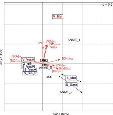
Microbial populations potentially involved in AOM pro-cesses co-varied with physicochemical conditions in the CIA performed on soft-sediment assemblages (Fig. 3, Table 4). The relationships were statistically significant (p = 0.01). According to the first axis, which contributed to 85 % of the variance, high methane and hydrogen sulfide concentra-tions and low sulfate concentraconcentra-tions were associated with high abundances of ANMEs 1 and 2 at one end, correspond-ing to S_Mat, V_Mat and S_Gast assemblages. The second axis, which accounted for 15 % of the variance, was driven by temperature anomalies and high NH4 concentrations at
V_Mat, where a higher frequency of ANME 1 and a lower frequency of ANME 2 and DSS were found compared with S_Mat and S_Gast. The first CIA axis thus summarised the variance due to chemosynthetic processes and can be consid-ered a proxy for fluid input across vent and seep ecosystems, whereas the second axis of the CIA summarised environmen-tal conditions that are specific to vents.
3.1.3 Foundation species descriptors
At seeps, E. spicata and L. barhami siboglinids showed max-imum size (368 mm) and biomass (457 g m−2), while the highest density was related to the small Hyalogyrina sp. gastropods (10 200 individuals per square metre (ind m−2); Table 5). At vents, R. pachyptila siboglinids had the max-imum size (431 mm), biomass (6630 g m−2) and density (1280 ind m−2). Siboglinid width, density and biomass were
much higher at vents than at seeps, while among the three vesicomyid assemblages, size, density and biomass were not statistically different.
3.2 Macrofaunal community structure 3.2.1 Density patterns
At seeps, macrofaunal densities ranged from 880 ind m−2 in S_Mat to ∼ 25 000 ind m−2 in S_Gast (Table 6). At vents, densities ranged from 710 ind m−2 in V_Mat to 94 400 ind m−2in V_Sib. The density at G_ref was the lowest with 570 ind m−2. Densities at the Guaymas reference, the seep assemblages and vent assemblages were significantly
d = 0.5 ANME_1 ANME_2 ANME_3 DSS DBB SRB2 G_ref S_VesP S_Sib_P S_Mat S_Gast S_VesA V_Mat V_VesA [CH4]max Tint Tmax [CH4]int [H2S] [Hint 2S]max [SO4]int [SO4]min [NH4]int [NH4]max Axis 1 (85%) Axis 2 (15%)
Figure 3. Co-inertia analysis of physicochemical factors in
soft-sediment assemblages: temperature, methane (CH4), hydrogen sul-fide (H2S), sulfate (SO4), ammonium (NH4) and relative abun-dances of microbial groups potentially involved in AOM: ANME1, ANME2, ANME3, DSS, DBB, SRB2. p = 0.01, axis 1 accounts for 85 % of the variation and axis 2 represents 15 %.
different (p = 0.03). Significant differences were found be-tween reference and seep densities (p < 0.05), whereas at vents, density was not significantly different either from seeps, or from the reference. Relatively comparable density ranges were observed across ecosystems for microbial mats and vesicomyid assemblages, whereas those of siboglinid as-semblages differed strongly, being higher at vents. Among the three vesicomyid assemblages, density differences were close to being significant (p = 0.07). Significant differences were found with higher densities at the seep A. gigas assem-blage (S_VesA) compared with the vent A. gigas (V_VesA) and seep P. soyoae (S_VesP) assemblages (p < 0.05), with the latter assemblages showing comparable densities.
Macrofaunal densities did not show any significant correlation with physicochemical factors. However, log-transformed densities showed that, along the range of max-imal methane concentrations, densities appeared to be en-hanced at seep and vent vesicomyid assemblages and seep siboglinids and their periphery compared with the reference, whereas the highest methane concentrations at seep and vent microbial mats were related to the minimum densities ob-served over all chemosynthetic assemblages (Fig. 4). In be-tween, high density fluctuations were found among vent alvinellid and vent siboglinid assemblages, despite relatively comparable maximal methane concentrations. A similar pat-tern was found between the seep gastropod assemblage and the seep and vent microbial mats. A polynomial
relation-Table 4. Quantitative PCR results for six Archaea and Bacteria phyla potentially involved in the anaerobic oxidation of methane (AOM):
ANME1, ANME2, ANME3, DSS, DBB and SRB2. Results are cumulated across the 0–10 cm sediment layer and expressed in 16S rRNA copy number per gram of sediment. The highest values for each group of AOM micro-organisms are shown in bold.
Abbreviation ANME1 ANME2 ANME3 DSS DBB SRB2
G_ref 8.16E+04 1.40E+06 2.74E+06 1.10E+08 4.08E+06 5.42E+05
S_VesP 3.84E+07 6.94E+07 2.32E+05 1.60E+08 4.88E+06 7.78E+06
S_VesA 1.28E+08 1.47E+08 3.42E+06 2.40E+08 4.44E+06 1.35E+06
S_Mat 7.84E+08 7.56E+08 1.45E+08 4.72E+08 4.00E+07 1.97E+07
S_Gast 1.12E+09 1.47E+09 3.38E+07 3.78E+08 5.28E+07 1.15E+07
S_Sib_P 5.10E+07 2.62E+08 1.65E+07 2.18E+08 3.62E+06 2.16E+06
V_VesA 2.34E+05 5.28E+05 2.42E+06 1.44E+08 5.80E+06 8.60E+05
V_Mat 1.09E+09 1.17E+08 1.33E+06 7.08E+07 6.36E+06 8.12E+07
Table 5. Characteristics of foundation species (size, density and biomass) in the Guaymas Basin. Standard deviations are given in parentheses
and highest values are shown in bold.
Species Length (L), diameter (D), Density Biomass
mm ind m−2 g m−2
Seep assemblages
S_Sib E. spicata/L. barhami L: 368 (116)/D: 6 (3) 721 457
S_VesA A. gigas L: 75.0 (8.9) 102 (42) 262 (119) S_VesP P. soyoae L: 87.1 (27.8) 74.1 (69.9) 405 (358) S_Gast Hyalogyrina sp. D: 2.0 (0.3) 10 170 2.4 Vent assemblages V_Sib R. pachyptila L: 431 (133)/D: 19.9 (9) 1280 6630 V_VesA A. gigas L: 57.0 (20.6) 55.6 (48.1) 81.3 (107)
V_Alv P. grasslei/P. bactericola L: 24.2 (14.4)/D: 2.2 (1.0) 1070 31.2
0 200 400 600 800 3.0 3.5 4.0 4.5 5.0 [CH4]max (µM) log10(Density) G_ref S_VesP S_Sib_P S_Sib S_Mat S_Gast S_VesA V_Mat V_Sib V_VesA V_Alv
Figure 4. Log-transformed macrofaunal densities according to
maximum methane concentrations in assemblages.
ship between macrofaunal community density and founda-tion species density was found with S_Gast and V_Sib as-semblages, harbouring higher densities of both foundation species and associated communities than the other assem-blages (R = 0.8, p < 0.05). No significant density differences were related to the nature of the substrata (soft versus hard substrata).
3.2.2 Alpha diversity patterns
As seen on rarefaction curves, the diversity was rela-tively well characterised depending on the assemblage. Four curves, corresponding to G_ref, V_VesA, V_Mat and S_Mat assemblages, did not reach an asymptote (Fig. 5), indicat-ing insufficient samplindicat-ing efforts. The samplindicat-ing efforts at V_Mat and G_ref was indeed relatively lower than at assem-blages where diversity was well characterised, but not at the V_VesA and S_Mat sites (Table 1).
ES(n) alpha diversity was estimated for each assemblage based on 41 individuals, corresponding to the minimum number of individuals observed at any one assemblage. ES41
Table 6. Macrofaunal community composition (expressed in terms of density: ind m−2)in the Guaymas Basin assemblages at the family level, including total densities (ind m−2)and ES41 diversity. Standard deviations are given in parentheses. The highest values for each assemblage are highlighted in bold.
G_ref S_VesP S_VesA S_Mat S_Gast S_Sib S_Sib_P V_VesA V_Mat V_Alv V_Sib
1 2 3 4 1 2 3 1 2 3 1 2 3 1 1 1 2 3 4 1 2 3 1 2 1 1 Bivalvia Bathyspinulidae 0 0 0 0 1778 361 83 1417 1583 972 333 28 111 0 144 556 167 333 111 167 222 417 0 0 0 0 Cuspidariidae 0 0 0 0 0 0 0 28 0 0 0 0 0 0 0 0 0 56 56 0 0 0 0 0 0 0 Mytilidae 0 0 0 0 0 0 0 0 0 0 0 0 0 0 86 0 0 0 0 0 0 0 0 0 0 71 Solemyidae 0 0 0 0 28 56 0 0 28 0 0 0 0 0 0 0 0 0 0 0 28 0 0 0 0 0 Thyasiridae 0 56 0 0 0 0 0 0 0 56 0 0 0 55.6 58 56 389 222 389 28 111 0 28 0 0 0 Gastropoda Aplustridae 0 0 0 0 0 0 0 0 0 28 0 0 0 0 58 0 0 0 0 28 0 0 0 0 0 0 Cataegidae 0 0 0 0 0 0 0 0 0 0 0 0 0 0 130 0 0 0 0 0 0 0 0 0 0 18 Hyalogyrinidae 0 0 0 0 28 0 0 0 0 28 0 0 0 0 0 0 0 0 0 0 0 0 0 0 0 0 Lepetodrilidae 0 0 0 0 0 0 0 0 0 0 0 0 0 0 2104 0 0 0 0 0 0 0 0 0 14 0 Neolepetopsidae 0 0 0 0 56 83 111 28 56 0 0 0 0 0 735 0 0 0 0 0 0 0 0 0 0 0 Neomphaloidae 0 0 0 0 0 0 0 0 56 0 0 0 0 0 0 0 0 0 0 0 250 28 0 0 0 0 Provannidae 0 0 0 0 167 167 0 56 0 0 0 0 0 0 43 0 0 0 0 417 28 0 0 28 0 0 Pyramidellidae 0 0 0 0 0 83 28 28 0 0 0 0 0 0 0 0 0 0 0 0 0 0 0 0 0 0 Pyropeltidae 0 0 0 0 0 0 0 0 28 0 0 0 0 0 0 0 0 0 0 0 0 0 0 0 0 0 Polychaeta Acoetidae 0 0 0 0 0 0 0 0 28 0 0 0 0 0 0 0 0 0 0 0 0 0 0 0 0 0 Ampharetidae 0 167 0 56 0 0 0 556 1806 56 806 0 28 17222 0 0 0 0 0 167 28 194 139 83 86 8269 Amphinomidae 0 0 0 0 0 0 0 28 0 0 0 0 0 0 0 0 0 0 0 0 0 0 0 0 0 0 Archinomidae 0 0 0 0 0 0 0 0 0 0 0 0 0 0 87 0 0 0 0 0 0 0 0 0 0 0 Capitellidae 0 0 56 0 56 0 0 0 83 0 0 0 0 0 0 111 0 0 0 0 0 0 0 0 0 0 Cirratulidae 167 278 56 167 28 28 167 444 194 1056 28 0 0 0 29 944 167 944 1444 111 56 28 0 0 0 0 Cossuridae 0 0 0 0 0 0 0 250 28 444 0 0 0 0 0 611 222 722 389 0 0 0 0 0 0 0 Dorvilleidae 0 0 0 0 28 28 167 6472 3889 2750 361 472 194 7611 231 556 1944 556 167 500 1389 111 444 611 1543 85946 Flabelligeridae 0 0 0 0 0 0 0 28 28 0 0 0 0 0 0 0 0 0 0 0 0 0 0 0 0 0 Glyceridae 0 0 0 56 28 0 0 28 0 0 0 0 0 0 0 56 0 111 0 28 0 0 0 0 0 0 Goniadidae 0 0 0 0 0 0 0 28 0 0 0 0 0 0 0 0 0 0 0 0 0 0 0 0 0 0 Hesionidae 0 0 0 56 0 0 0 1278 583 167 111 0 28 0 0 444 444 111 111 83 0 0 28 0 0 0 Lacydonidae 0 0 0 0 0 0 0 278 0 56 0 0 0 0 0 0 0 56 0 0 0 0 0 0 0 0 Lumbrineridae 0 0 0 0 0 0 28 361 139 250 0 0 0 0 43 833 167 56 1000 28 0 0 0 0 0 0 Maldanidae 0 0 0 0 28 0 56 56 56 28 0 0 0 0 43 56 0 0 0 0 0 0 0 0 0 0 Nautiliellidae 0 0 0 0 0 56 0 0 28 0 0 0 0 0 0 0 0 0 0 0 0 0 0 0 0 0 Nephtyidae 0 0 0 0 0 0 0 0 0 111 0 0 0 0 0 0 0 0 0 0 0 0 0 0 0 0 Nereididae 56 222 0 0 0 0 0 83 194 28 0 0 0 0 259 0 0 0 0 28 0 0 56 0 0 0 Opheliidae 0 0 0 0 0 0 0 0 0 0 0 0 0 0 0 0 0 0 56 0 0 0 0 0 0 0 Paraonidae 167 56 56 0 0 0 0 167 0 222 0 0 0 0 0 444 389 444 333 0 0 0 0 0 0 0 Pholoidae 0 56 0 0 0 0 0 28 0 28 0 0 0 0 0 0 0 56 0 0 0 0 0 0 0 0 Phyllodocidae 0 0 0 0 0 0 0 0 0 0 0 0 0 0 332 0 0 0 0 0 0 0 0 0 0 0 Pilargidae 0 0 111 0 0 0 0 56 0 83 0 0 0 0 0 0 0 0 167 0 28 0 0 0 0 0 Polynoidae 0 0 0 0 0 0 0 28 0 83 28 0 0 0 1629 0 0 111 56 0 0 0 0 0 971 18 Serpulidae 0 0 0 0 0 0 0 0 0 0 0 0 0 0 1485 0 0 0 0 0 0 0 0 0 0 0 Sigalionidae 0 56 0 56 0 0 0 0 0 28 0 0 0 0 0 56 0 56 56 0 0 0 0 0 0 0 Sphaerodoridae 0 0 0 0 0 0 0 139 83 83 0 0 0 0 14 0 0 0 0 28 0 0 0 0 0 0 Spionidae 56 111 0 0 0 0 0 28 56 83 0 0 0 0 43 222 0 56 111 0 0 0 0 0 0 0 Sternaspidae 0 0 0 0 0 0 0 28 0 28 0 0 0 0 0 0 0 0 0 0 0 28 0 0 0 0 Syllidae 0 0 0 0 0 0 0 0 0 0 0 27 0 0 0 0 0 0 0 0 0 0 0 0 0 0 Terebellidae 0 0 0 0 139 0 0 56 28 0 0 0 0 0 404 0 0 111 0 0 0 0 0 0 0 0 Trichobranchidae 0 0 0 0 0 0 0 0 0 28 0 0 0 0 0 0 0 0 56 0 0 0 0 0 0 0 Others Actinaria 0 56 0 0 0 56 0 83 0 0 0 0 0 0 0 0 56 0 0 0 0 0 0 0 0 0 Amphipoda 0 0 0 0 0 0 0 0 56 28 0 0 0 0 29 56 0 0 0 333 28 0 0 0 0 26 Aplacophora 0 0 56 56 0 0 56 1250 917 222 28 0 0 0 14 56 0 56 0 0 56 28 0 0 0 0 Cnidaria 0 0 0 0 0 0 0 28 28 0 0 0 0 0 0 0 0 0 0 0 0 0 0 0 0 Cumacea 0 0 0 0 0 0 0 0 0 0 56 0 0 0 0 0 0 0 0 0 0 0 0 0 0 0 Nemertina 0 0 0 0 0 0 0 194 389 56 0 0 0 0 0 0 167 0 0 0 0 0 0 0 0 0 Ophiuridae 0 0 0 0 83 194 28 306 861 833 0 0 0 0 29 0 0 56 0 0 0 0 0 0 0 0 Scaphopoda 0 0 0 0 0 0 0 0 0 0 0 0 0 0 0 111 0 0 0 0 0 0 0 0 0 0 Sipuncula 0 0 0 0 0 0 0 167 28 0 0 0 0 0 0 0 0 0 0 0 0 0 0 0 0 0 Tanaidacea 0 0 0 0 0 0 0 0 28 0 0 0 0 0 0 611 0 56 56 0 0 0 0 0 0 0 Mean density 569 (328) 1426 (903) 11 037 (3090) 880 (762) 24 889 8028 4653 (776) 1667 (735) 708 (20) 2614 94 348 ES41 14 11.1 12.2 6.4 2.1 10.9 12.9 10.3 5.4 3 2
and from 2 (V_Sib) to 10 families (V_VesA) at vents, while the reference included 14 families (G_ref, Table 6).
Alpha diversity appeared maximal at the Guaymas ref-erence (as observed with ES(n) and the rarefaction curve) and was not significantly different among seeps and vents. Relatively comparable ES41values were observed in
micro-bial mat and vesicomyid vent and seep assemblages, whereas they showed strong differences in siboglinid assemblages, with lower diversity at the vent one. Although ES41did not
separate the three vesicomyid assemblages, the rarefaction
curves showed higher diversity in the seep A. gigas assem-blage compared with the seep P. soyoae assemassem-blage. The di-versity in the vent A. gigas assemblage was not sufficiently characterised, but appeared to be intermediate between the two vesicomyid seep assemblages (Fig. 5).
A negative correlation was observed between ES41 and
temperature anomalies (R > 0.6, p < 0.05), reflecting that three of the four vent assemblages showed relatively low diversity, whereas four of the six seep assemblages had relatively high diversity. A strong negative correlation was
0 200 400 600 800 1000 1200 0 10 20 30 40 Number of individuals Expected richness G_ref S_VesP S_Sib_P S_Sib S_Mat S_Gast S_VesA V_Mat V_Sib V_VesA V_Alv ...
Figure 5. Rarefaction curves on pooled macrofaunal abundances
from each assemblage.
found between ES41 and methane concentrations for all
as-semblages (R > 0.8, p < 0.01). ES41 on soft-sediment
as-semblages was positively correlated with sulfate concentra-tions and negatively correlated with hydrogen sulfide and methane concentrations (R > 0.7, p < 0.05). In addition, a linear regression model was fit to the relationship between ES41and maximum methane concentrations, previously
log-transformed, among all assemblages to compare our data with previous studies. This regression was highly significant (R2=0.78, p < 0.001) and reflected a decrease in diversity along a fluid input gradient (Fig. 6).
3.2.3 Community composition patterns
Macrofaunal community composition varied both within and between ecosystems. The relative abundances of macrofau-nal taxa within assemblages are presented in Fig. 7 and their inter-assemblage variability in Fig. 8.
All macrofaunal communities were dominated by Poly-chaeta at the reference (90.2 %), at seeps (from 57.3 to 99.8 %), with the exception of S_VesP where Bivalvia dom-inated (53.9 %) and at vents (from 56.7 to 99.9 %). At the family level, a strong inter-assemblage variability was ob-served. The three first axes of the between-group PCA, a particular case of RDA that tests and maximises the vari-ance between assemblages, accounted for 51 % of the total variance in community composition. The intra-assemblage heterogeneity was relatively high, but lower than the inter-assemblage variability, with the exception of S_VesA and V_VesA in which there was a slight overlap. The first axis of the PCA accounted for 27 % of the variability in commu-nity composition, mostly separating the G_ref and S_Sib_P assemblages dominated by Cirratulidae, Paraonidae and Spi-onidae polychaetes from the V_Sib, V_Mat, V_Alv, S_Gast
0.0 0.5 1.0 1.5 2.0 2.5 3.0 2 4 6 8 10 12 14 G_ref S_VesP S_Sib_P S_Sib S_Mat S_Gast S_VesA V_Mat V_Sib S_VesA V_Alv Log[CH4]max (µM) ES(41)
Figure 6. Logarithmic regression between species richness, ES(41),
and maximum methane concentration in all macrofaunal assem-blages. Black squares represent observed data points and red squares represent fitted values.
and S_Mat assemblages, characterised by higher frequencies of Dorvilleidae and Ampharetidae polychaetes. Intermediate compositions were found at S_Sib_P, S_VesP, S_VesA and V_VesA. The second axis accounted for 14 % of the variance in macrofaunal community composition. It was mainly influ-enced by the dominance of the Bathyspinulidae bivalves at S_VesP. The third axis accounted for 10 % of the variance, differentiating in particular the S_Sib assemblage, charac-terised by the presence of Polynoidae, Lepetodrilidae, Ne-olepetopsidae, Serpulidae and Nereididae.
Overall, although the heterogeneity between macrofaunal communities appeared higher at seeps than at vents, there was no differentiation between vent and seep assemblages. Community compositions across seep and vent common mi-crobial mats and vesicomyid assemblages were closely re-lated, whereas they differed according to the ecosystem they belonged to among siboglinid assemblages. Of the three vesi-comyid assemblages, those dominated by A. gigas at seeps and vents were more similar than those dominated by P.
soyoae in seeps.
Relationships with site characteristics
The forward selection test showed that the variation of macrofaunal community composition among assemblages was significantly influenced by maximum methane concen-trations and the type of substratum (p < 0.01), whereas tem-perature anomalies and the biomass and density of foun-dation species were not significant. The first two compo-nents of the canonical redundancy analysis (RDA) accounted for respectively 27 % (p = 0.01) and 13 % (p = 0.08) of the variability in macrofaunal composition (adjusted R2,
0 10 20 30 40 50 60 70 80 90 100%
G_ref S_VesP S_Sib_P S_Sib S_Mat S_Gast S_VesA V_Mat V_Sib V_VesA V_Alv
Dorvilleidae Bathyspinulidae Ampharetidae Aplacophora Hesionidae Ophiuridae Cirratulidae Lumbrineridae Cossuridae Nemertina Paraonidae Lacydonidae Lepetodrilidae Polynoidae Serpulidae Neolepetopsidae Terrebellidae Phyllodocidae Nereididae Cumacea Cataegidae Mytilidae Archinomidae Thyasiridae Tanaidacea Spionidae Syllidae Solemyidae Sigalionidae Pyramidellidae Provannidae Pilargidae Pholoidae Neomphaloidae Nautiniellidae Maldanidae Glyceridae Capitellidae Amphipoda Actinaria Others
Figure 7. Histograms of relative macrofaunal compositions at the family level in assemblages shown for each study site; only taxa
contribut-ing to more than 1 % are shown.
Lepetodrilidae Neolepetopsidae Bathyspinulidae Thyasiridae Vesicomyidae Ampharetidae Cirratulidae Cossuridae Hesionidae Lumbrineridae Nereididae Paraonidae Polynoidae Serpulidae Spionidae Tanaidacea G_Ref V_Sib V_Mat V_VesA V_Alv S_VesP S_Sib_P S_Sib S_Gast S_Mat S_VesA Dorvilleidae Axis 1 (27%) Axis 3 (10%) G_Ref V_Sib V_Mat V_VesA V_Alv S_VesP S_Sib_P S_Sib S_Gast S_Mat S_VesA Neolepetopsidae Provannidae Bathyspinulidae Ampharetidae Cirratulidae Dorvilleidae Paraonidae Spionidae Ophiuridae Dorvilleidae Axis 1 (27%) Axis 2 (14%) (a) (b)
Figure 8. Between-group principal component analysis (PCA) on Hellinger-transformed macrofaunal densities of the 26 sampling units
studied in the Guaymas Basin. (a) The axis 1 accounts for 27 % of the variance in the macrofaunal data and axis 2 accounts for 14 %. (b) The axis 1 accounts for 27 % of the variance in the macrofaunal data and axis 3 accounts for 10 %. Only taxa contributing to more than 2 % to an axis are shown.
0.25; Fig. 9). The first axis was mostly driven by maximum methane concentrations. The high methane concentrations at the S_Gast, V_Sib, V_Mat, V_Alv and S_Mat habitats were mainly associated with the dominance of dorvilleids and ampharetids and to a lesser extent to polynoids. The low methane concentrations at all other habitats were linked to higher abundances of cirratulids, bathyspinulids, paranoids,
lumbrinerids, aplacophorans, ophiurids, hesionids and ne-olepetopsids. Nevertheless, in this latter group, S_VesA and V_VesA compositions had more affinities with assemblages characterised by high methane concentrations. The second RDA axis was driven by the type of substratum (hard/soft) but also by higher methane concentrations in V_Mat, S_Mat and S_Gast habitats. At one axis end, hard substrata mainly
Figure 9. Canonical redundancy analysis (RDA, scaling type 1) of
Hellinger-transformed macrofaunal densities as a function of qual-itative and normalised quantqual-itative environmental conditions for all assemblages (a) or for soft-sediment assemblages (b). Only signifi-cant explanatory variables are shown (a) methane concentration and substratum type; (b) first axis of the prior co-inertia analysis and engineer species biomass). Only the names of the taxa that showed good fit with the first two canonical axes (fitted value > 0.20) are shown on the plots.
contributed to S_Sib and V_Alv macrofaunal composition, with the presence of polynoids at V_Alv coupled to that of lepetodrilids, serpulids and neolepetopsids at S_ Sib. At the other axis end, the higher methane concentrations in V_Mat, S_Mat and S_Gast mainly accounted for the higher domi-nance of ampharetids whereas soft substrata appeared to ex-plain the abundance of hesionids and bathyspinulids.
Focusing on soft-sediment assemblages, the forward se-lection test showed that macrofaunal community composi-tion was significantly influenced by the first axis of the co-inertia analysis (CIA) and the biomass of foundation species, which were the best explanatory variables (p values of 0.01 and 0.07, respectively). The relationship with the first axis of the CIA, which we interpreted as a proxy for fluid in-put across ecosystems, was highly significant, whereas the relationship with the second axis of the CIA, which we interpreted as being vent-specific, was not. The first two components of the RDA accounted for respectively 31 % (p = 0.03) and 20 % (p = 0.06) of the variability in macro-faunal composition (adjusted R2=0.31; Fig. 9). Accord-ing to the first axis, higher fluid inputs at S_Mat, V_Mat, S_Gast contributed to the high dominance of ampharetids and dorvilleids. At the other end, all other assemblages were characterised by a higher proportion of taxa from the Cir-ratulidae and Bathyspinulidae families. In this latter group, S_VesA, V_VesA assemblages were found to have more affinities with assemblages of high fluid input than the other assemblages. The second axis was mainly driven by the biomass of foundation species, distinguishing S_VesP from the other assemblages with high frequencies of nuculanid bi-valves, ophiurids, and gastropods compared with lower fre-quencies dominance of several polychaete families. This pat-tern may also be related to differences in the engineering ef-fects of P. soyoae at S_VesP, compared to A. gigas, at S_VesA and V_VesA.
3.2.4 Faunal composition similarity between seep and vent ecosystems
At the family level, the gamma diversity of macrofaunal com-munities reached 56 families at the seep ecosystem, 22 fami-lies at vent ecosystem and 14 at the reference. All the famifami-lies found at the reference were also found at the seep and eight of them were shared with the vent. As the diversity at the ref-erence was estimated from only one assemblage, its faunal similarity/dissimilarity to seep and vent ecosystems was not quantified. Between seep and vent macrofaunal composition, the Sorensen dissimilarity was estimated at 42 % and corre-sponded only to nestedness (species loss), whereas the dis-similarity linked to turnover (species replacement) was null. All the 22 families found at vent were also found at seep with seep exhibiting 28 specific families and 6 families only shared with the reference.
In all, 26 species belonging to 18 seep and vent dominant families were identified (Table 7). Of these, the vast majority (22 species) were found in both ecosystems, whereas only two species of gastropods were specific to seep (Eulimella
lomana and Paralepetopsis sp.) and two were restricted to
vent (the polynoid Branchiplicatus cupreus and the gastro-pod Pyropelta musaica).
Table 7. Presence or absence of seep and vent species in the Guaymas Basin (∗: species not found within our study but previously recorded in Guaymas vents) and species records from other studies in the Costa Rica “hydrothermal seep” (CRHS) and, more generally, at cold seeps (CS), vents (HV) or organic falls (OF) around the world.
Guaymas Guaymas CRHS CS HV OF References
Seep Vent
Foundation species
Phreagena soyoae x x∗ x x x Baco et al. (1999); Audzijonyte et al. (2012)
Archivesica gigas x x x x x x Krylova and Sahling (2010); Audzijonyte et al. (2012); Smith et al. (2014); Levin et al. (2012a)
Calyptogena pacifica x x x x Huber (2010); Audzijonyte et al. (2012); Smith et al. (2014)
Paralvinella bactericola x Desbruyères and Laubier (1991)
Paralvinella grasslei x x Desbruyères and Laubier (1982); Zal et al. (1995)
Riftia pachyptila x x Black et al. (1994)
Escarpia spicata x x∗ x x x Black et al. (1997); Levin et al. (2012a); Feldman et al. (1998);
Tunnicliffe (1991)
Lamellibrachia barhami x x x x Black et al. (1997); Levin et al. (2012a)
Hyalogyrina sp. x genus genus genus genus Smith and Baco (2003); Bernardino et al. (2010); Smith et al. (2014); Sahling et al. (2002); Sasaki et al. (2010); Levin et al. (2012a) Associated macrofauna
Nuculana grasslei x x Allen (1993)
Acharax aff. johnsoni x x x Kamenev (2009)
Sirsoe grasslei x x Blake and Hilbig (1990)
Ophryotrocha platykephale x x x x Weiss and Hilbig (1992); Levin et al. (2003); Smith et al. (2014)
Ophryotrocha akessoni x x x Blake and Hilbig (1990)
Parougia sp. x x genus genus genus Smith and Baco (2003); Bernardino et al. (2010); Levin et al. (2003); Levin (2005); Smith et al. (2014)
Exallopus jumarsi x x Petrecca and Grassle (1990)
Branchinotogluma sandersi x x x Blake and Hilbig (1990)
Branchinotogluma hessleri x x x Blake and Hilbig (1990)
Bathykurila guaymasensis x x x Pettibone (1993); Smith and Baco (2003); Blake and Hilbig (1990); Blake (1990); Smith (2003)
Branchiplicatus cupreus x x Blake and Hilbig (1990)
Nereis sandersi x x x Blake and Hilbig (1990)
Nicomache venticola x x x Blake and Hilbig (1990)
Aphelochaeta sp. x x genus Levin et al. (2003)
Sigambra sp. x x genus x Levin and Mendoza (2007); Dahlgren et al. (2004)
Amphisamytha aff. fauchaldi x x x x Stiller et al. (2013)
Parvaplustrum sp. x x
Provanna sp. (spiny) x x x Levin et al. (2012a)
Provanna laevis x x x x Sahling et al. (2002); Sasaki et al. (2010); Smith and Baco (2003);
Levin and Sibuet (2012); Levin et al. (2012a); Warén and Bouchet (1993)
Retiskenea diploura x x x Sahling et al (2002); Sasaki et al. (2010)
Eulimella lomana x x∗ x x x Sahling et al. (2002); Sasaki et al. (2010); Smith and Baco (2003); Levin and Sibuet (2012); Levin et al. (2012a); Warén and Bouchet (1993)
Lepetodrilus guaymasensis x x x Levin et al. (2012a); Sasaki et al. (2010)
Pyropelta corymba x x x x x Sasaki et al. (2010); Levin et al. (2012a); Smith and Baco (2003)
Pyropelta musaica x x x x Smith and Baco (2003); Tunnicliffe (1991); Sasaki et al (2010)
Paralepetopsis sp. x genus genus genus Sasaki et al. (2010)
Cataegis sp. x x genus genus Levin et al. (2012a;) Sasaki et al. (2010)
4 Discussion
Previous comparative studies have highlighted strong dif-ferences between seep and vent macrofaunal communities (Bernardino et al., 2012; Tunnicliffe et al., 2003, 1998; Sibuet and Olu, 1998; Turnipseed et al., 2003 2004; Watan-abe et al., 2010; Nakajima et al., 2014). However, to date, large-scale ecological factors and biogeographic bar-riers have limited any direct comparisons of the impact of seep- and vent-specific environmental conditions. Although methane and hydrogen sulfide appear to be potential com-mon structuring factors across seep and vent ecosystems,
ecosystem-specific fluid properties may further shape com-munity patterns. In addition, other environmental factors such as the type of substratum and the role of foundation species as engineers could potentially add complexity within communities (Govenar, 2010; Cordes et al., 2010).
4.1 Similarities and differences in site biogeochemistry Substratum
Both Guaymas chemosynthetic ecosystems showed typical faunal assemblages colonising hard (seep: siboglinid, vent:
siboglinid, alvinellid) and soft substrata (seep: vesicomyid, gastropod and microbial mat, vent: vesicomyid and microbial mat). The nature of hard substratum differed among ecosys-tems with authigenic carbonates at seeps (Paull et al., 2007) and sulfide edifices at vents (Jørgensen et al., 1990).
Vent and seep physicochemical conditions
Methane and hydrogen sulfide used as fluid input proxies had similar concentration ranges in seep and vent ecosys-tems. Seep and vent assemblages were divided in two groups, regardless of the ecosystem: those with low fluid inputs (seep siboglinid and periphery and seep and vent vesicomyid assemblages) and those with high fluid inputs (seep and vent microbial mat, seep gastropod, vent siboglinid and vent alvinellid assemblages). In addition, two of the three seep and vent common assemblages (vesicomyid and microbial mat) showed relatively comparable fluid inputs. Microbial mat assemblages are indeed usually characterised by strong fluid inputs, whereas vesicomyid habitats are related to lower fluid inputs (Levin, 2005). The third common assemblage did not exhibit the same pattern: the vent siboglinid habitat was associated with much higher fluid inputs than seep habitat. Siboglinid species at seeps and vents tend to occupy differ-ent ecological niches along a gradidiffer-ent of fluid flux. The seep
L. barhami and E. spicata siboglinids pump hydrogen sulfide
through their roots deep in the sediment in low-flux settings (Julian et al., 1999) and the vent taxon R. pachyptila captures the chemical elements through its gills, in stronger fluid flux conditions (Arp and Childress, 1983).
In sediment-covered vent fields, fluid emissions at the water–substratum interface may differ strongly from the original end-member fluids and potentially lead to reduced seep and vent environmental discrepancies, as shown else-where in terms of temperature and geochemistry (Sahling et al., 2005; Tunnicliffe et al., 2003; LaBonte et al., 2007; Von Damm et al., 1985). Although the Guaymas seep and vent habitats shared comparable ranges of methane and hydrogen sulfide concentrations, vents showed temperature anomalies correlated to the fluid inputs, ranging from 6.5◦C in the vesi-comyid assemblage to 55.5◦C in the microbial mat. Vents were also characterised by higher ammonium concentrations, lower pH and higher manganese concentrations than seeps, reflecting the end-member concentration of the vent fluids (Von Damm et al., 1985). Vent enrichment in ammonium is related to the thermocatalytic percolation of sedimentary or-ganic matter by hydrothermal fluids, a process that produces methane and petroleum-like aliphatic and aromatic hydrocar-bons (Bazylinski et al., 1988; Von Damm et al., 1985; Pear-son et al., 2005; Simoneit et al., 1992).
Vent-specific factors such as temperature, metals, pH and petroleum-like hydrocarbons may limit fauna, but not much is known about them. Although metal concentrations in Guaymas vent fluids are known to be lower than typical basalt-hosted systems – presumably due to the high
alkalin-ity and high pH of the fluids that reduce metal solubilalkalin-ity (Von Damm et al., 1985) – heavy metals may be potentially toxic in minute quantities (Decho and Luoma, 1996). In addition, a comparative study of the Guaymas and 9◦500N vents in the East Pacific Rise (EPR) showed that concentrations in metals were lower in vent fluids but higher in organism tis-sues at Guaymas (Von Damm, 2000; Von Damm et al., 1985). This suggests that heavy metal bioaccumulation is indepen-dent of the total metal concentrations, and depends on metal bioavailability (Ruelas-Inzunza et al., 2003; Demina et al., 2009).
AOM-related microbial populations
AOM has been shown to represent a major microbial pro-cess within both Guaymas cold seeps (Vigneron et al., 2013, 2014) and hydrothermal vents (Teske et al., 2002; Dhillon et al., 2003, 2005; Holler et al., 2011; Biddle et al., 2012). In our study, the composition of microbial communities potentially involved in AOM processes co-varied with physicochemi-cal conditions among soft-sediment habitats. Variations were mainly related to higher ANME archaeal abundance at both seep and vent high fluid-flux habitats. Both ANME1 and ANME2 dominance increased with fluid flux intensity and thus contrast with patterns observed at the hydrate ridge methane seeps (Marlow et al., 2014a, b). There, sediment and carbonate ANME communities were related to higher dominance of ANME2 in high fluid-flux compared to low fluid-flux habitats whereas ANME1 showed the opposite pat-tern. Nevertheless, within our study, compositions of ANME clades were distinct between seep and vent high fluid-flux as-semblages: ANME1 dominated at vent microbial mat blage, whereas seep microbial mats and gastropod assem-blages showed co-dominance of ANME1 and 2. These re-sults support previous studies suggesting that ANME1 is as-sociated with higher temperatures and potentially more per-manent anoxic environments compared to ANME2 (Rossel et al., 2011; Biddle et al., 2012; Vigneron et al., 2013; Holler et al., 2011; Nauhaus et al., 2005).
Foundation species
Foundation species may add heterogeneity within and be-tween ecosystems through both allogenic and autogenic en-gineering (Govenar, 2010; Cordes et al., 2010). The tubes of siboglinid worms and the shells of bivalves can pro-vide substratum and increase habitat complexity, promot-ing settlement or survivorship of associated species (Gove-nar, 2010). Vesicomyids that move vertically and laterally and, to a lesser extent, gastropods that can reach exception-ally high densities, may rework sediments, thus increasing oxygen penetration depth and indirectly promoting sulfide production (Wallmann et al., 1997; Fischer et al., 2012). In seep habitats, siboglinid tubeworms can also stimulate fide production through bio-irrigation and the release of