Analysing plant-pollinator interactions with spatial movement networks

HAL Id: hal-02105102

https://hal.archives-ouvertes.fr/hal-02105102

HAL is a multi-disciplinary open access archive for the deposit and dissemination of sci-entific research documents, whether they are pub-lished or not. The documents may come from teaching and research institutions in France or abroad, or from public or private research centers.

L’archive ouverte pluridisciplinaire HAL, est destinée au dépôt et à la diffusion de documents scientifiques de niveau recherche, publiés ou non, émanant des établissements d’enseignement et de recherche français ou étrangers, des laboratoires publics ou privés.

Analysing plant-pollinator interactions with spatial

movement networks

Cristian Pasquaretta, Raphaël Jeanson, Christophe Andalo, Lars Chittka,

Mathieu Lihoreau

To cite this version:

Cristian Pasquaretta, Raphaël Jeanson, Christophe Andalo, Lars Chittka, Mathieu Lihoreau. Analysing plant-pollinator interactions with spatial movement networks. Ecological Entomology, Wi-ley, 2017, Entomological Networks: Ecology, Behaviour and Evolution, 29th Symposium of the Royal Entomological Society, 42 (S1), pp.4-17. �10.1111/een.12446�. �hal-02105102�

1

Analysing plant-pollinator interactions with spatial

1

movement networks

2 3

Cristian Pasquaretta1*_{, Raphaël Jeanson}1_{, Christophe Andalo}2_{, Lars Chittka}3*_{, Mathieu Lihoreau}1

4 5

1_{Research Center on Animal Cognition, Center for Integrative Biology, Toulouse University, CNRS,}

6

UPS, France 7

2_{Laboratoire Evolution et Diversité Biologique (EDB), Université Toulouse III Paul Sabatier, F-31062}

8

Toulouse, France 9

3_{Department of Biological and Experimental Psychology, School of Biological and Chemical Sciences,}

10

Queen Mary University of London, Mile End Road, London E1 4NS, UK. 11

12

*Corresponding authors: 13

Lars Chittka - email: [email protected] 14

Cristian Pasquaretta – email: [email protected] 15

16 17 18

2

Abstract

19

1) Pollinators, such as bees, face the complex challenge of efficiently exploiting patchily distributed 20

floral resources across large landscapes. 21

22

2) Here we consider the utility of spatial network statistics for analysing the foraging patterns of bees 23

moving between feeding sites at various spatial and temporal scales. 24

25

3) First we explain how spatial movement networks can be derived theoretically and experimentally to 26

describe bee foraging decisions. 27

28

4) We then illustrate this approach by analysing six datasets of bumblebees and honeybees foraging 29

in arrays of artificial flowers, and showing how some specific network metrics vary predictably as 30

foragers gain experience with the spatial distribution of feeding sites. 31

32

5) We compare network analyses to more conventional statistics used to characterise bee foraging 33

movements and discuss the implications of this novel statistical and modelling approach for pollination 34

ecology research. 35

36

Keywords: bumblebees; foraging; honeybees; movement ecology; pollination; route optimization; 37 spatial networks. 38 39 40 41 42 43

3

Introduction

44

Bees play a key role in the reproduction of wild and cultured plants. Over recent years, their 45

widespread declines have raised considerable concern for food security and the sustainability of our 46

ecosystems (Goulson et al., 2015; Klein et al., 2017). Central to understanding the impact of pollinator 47

loss on plant reproduction is the foraging behaviour of bees (Thomson, 1986; Waser, 1986). Most 48

bees are central-place foragers, meaning that they collect food (nectar and pollen) to provision their 49

brood in a single nest (Michener, 2000). By exploiting plants and developing foraging routes to visit 50

them, individual bees may bias pollen flow and fashion the genetic structure of plant populations, 51

therefore calling for more research of bee spatial strategies at the individual and collective levels 52

(Ohashi & Thomson, 2009; Burkle & Alarcón, 2011; Mayer et al., 2011). 53

Historically, bees were assumed to use simple movement rules that would yield maximal 54

energy gains to exploit patchily distributed resources, such as moving between nearest unvisited 55

flowers (Ohashi et al., 2007), making short trips after encountering highly rewarding flowers (Chittka et 56

al., 1997) or keeping constant heading directions between visiting flowers (Pyke & Cartar, 1992). 57

While these rules of thumb may hold true when bees forage at small spatial scales (within an 58

inflorescence or a flower patch) mounting evidence shows that this is not the case at larger spatial 59

scales, when bees move between distant locations (flower patches or plants). In these conditions, 60

foragers of many bee species tend to develop stable foraging routes (sometimes called traplines in 61

analogy to the fixed circuits that trappers follow when examining a number of traps distributed widely 62

in space) that they follow for several hours or days (e.g. Euglossine bees: Janzen, 1971; bumblebees: 63

Heinrich 1976; Thomson et al., 1997; honeybees: Buatois & Lihoreau, 2016). This routing behaviour is 64

based on the acquisition of spatial memories encoding the location of the different food resources, the 65

colony nest site and other prominent environmental features (e.g. visual landmarks) (Collett et al., 66

2013). With training, bumblebees and honeybees can learn to find the shortest path to visit a few 67

artificial flowers (equivalent to natural flower patches) once and return to the nest (Bombus impatiens: 68

Ohashi et al., 2007; Bombus terrestris: Lihoreau et al., 2012a; Apis mellifera: Buatois & Lihoreau, 69

2016), an optimisation behaviour analogous to solving the Travelling Salesman Problem in graph 70

theory (Cook, 2012). This mathematical problem is notoriously difficult (if not impossible) to solve for 71

large graphs, because the number of possible paths increases factorially with the number of nodes in 72

the graph (e.g. 6 paths for 3 nodes, > 3 million paths for 10 nodes), and finding efficient solutions often 73

requires complex algorithms and systematic approaches (Polyakovskiy et al., 2014; Dorigo & 74

Gambardella, 2016). 75

While there is evidence that bees exhibit routing behaviour in nature (Heinrich 1976; Janzen 76

1971), to what extent these observations in simplified experimental conditions can be extrapolated to 77

the field, where individuals may interact to exploit numerous highly variable resources scattered 78

across large landscapes, is an open question. 79

Field data on such multi-destination routes among flower patches are even more complex and 80

challenging to analyse, and conventional behavioural metrics do not suffice to capture detailed 81

information about routing behaviour (Thomson et al., 1997; Makino & Sakai 2004; Makino & Sakai 82

2005; Makino 2013; Lihoreau et al., 2016). We argue that network statistics derived from graph theory 83

4

hold considerable promise to characterise these complex movement patterns at the individual and 84

collective levels, and to identify the decision rules underpinning spatial strategies. In developing routes 85

between flowers, foragers form movement networks embedded in space (Barthélemy, 2011), where 86

‘nodes’ are feeding locations (flower patches or plants) and ‘edges’ are flight paths between them (see 87

examples in Figures 1A-E) (Thomson et al., 1997; Lihoreau et al., 2016). These spatial movement 88

networks are directed, meaning that individuals move from one particular location to another 89

(movement vectors). Networks are also weighted so that the thickness of edges is proportional to the 90

frequency of movements between nodes. Because most bee species are central-place foragers, their 91

spatial movement networks also include the nest site, a specific node at which every flower visitation 92

sequence starts and ends. Therefore, in principle, an optimal movement network for a bee connects all 93

flowers and the nest using the shortest possible path (optimal network in Figure 1E). Discrete temporal 94

network analysis can then be performed depending on the time intervals with which a visitation matrix 95

is built. For instance, matrices may be developed by considering flower visits made in a single foraging 96

bout (dynamic network) or by cumulating the flower visits of several foraging bouts (static network). A 97

major advantage of network statistics is that they allow for analyses of very large spatial datasets and 98

the derivation of new empirically testable hypotheses (e.g. Perna & Latty, 2014; Jacoby & Freeman, 99

2016). Several analytical packages (e.g. igraph, sna, tnet packages in R, graph-tool in Python, 100

UCINET) and both local metrics (e.g. measures describing the level of importance of a node in a 101

network) and global metrics (e.g. measures describing the general level of connectivity of the entire 102

network) can be readily calculated to characterize space use by pollinators from an individual-based 103

point of view to measure, compare and predict their behaviour across different temporal scales. 104

In a recent field survey, Dupont et al. (2014) applied an individual-based plant-pollinator 105

network analysis to flower visitation data of different bumblebee species. The study showed significant 106

modularity in space use by bees based on plant characteristics, so that foragers tended to visit 107

patches of aggregated plants with numerous flowers and use taller plants to move from one module to 108

another (Dupont et al., 2014). Although the analytical approach developed in this study is very 109

appealing, field surveys only provide partial information about the foraging experience of individual 110

bees, the location of their nest relative to different plant patches and the temporal dynamics of their 111

foraging patterns. All these parameters are critical in determining bee foraging behaviour (Chittka & 112

Thomson, 2001). Experimental advances on model bee species, such as bumblebees and 113

honeybees, using artificial flowers delivering controlled rates of food resources combined with 114

automated movement tracking, now allow for collecting high resolution spatial and temporal data on 115

bee foraging patterns in complex, yet controlled, environments (e.g. motion detection cameras on 116

flowers: Lihoreau et al., 2016; Radio Frequency Identification (RFID): Ohashi et al., 2010; harmonic 117

radars: Lihoreau et al., 2012b; QR tags: Crall et al. 2015; 3D video tracking: Ings & Chittka, 2008). 118

Extensive recordings of individual based data using these semi-field approaches provide an 119

interesting opportunity to start examining the cognitive processes underpinning the foraging patterns 120

of bees and how they change across time in ecologically relevant conditions. 121

Here we describe how spatial network statistics can be used to analyse the foraging patterns of 122

bees both at local and global levels. We illustrate the potential of this approach for comparative analyses 123

5

by statistically comparing spatial optimisation in the movement patterns of bees of the same species or, 124

of different species across environments varying in spatial scales, number of flowers and flower 125

configurations using standard network metrics. We used published movement datasets of bumblebees 126

and honeybees of known age, foraging experience and colony origin, foraging in arrays of artificial 127

flowers in the lab and in the field. To validate the approach, we compared our results with analyses of 128

more conventional behavioural metrics used in previous studies, such as the number of re-visits to 129

flowers and overall travel efficiency (distance/number of flowers visited). 130

131

Materials and methods

132

Experimental data 133

We analysed six datasets of bee flower visitation sequences. Three datasets were obtained on the 134

bumblebee Bombus terrestris (experiment 1: Lihoreau et al., 2012a; experiment 2: Lihoreau et al., 135

2011; experiment 3: Lihoreau et al., 2012b). The three other datasets were obtained on the honeybee 136

Apis mellifera (experiments 4-6: Buatois & Lihoreau, 2016). 137

All the datasets were generated following the same general methodology and are thus 138

comparable. In all experiments bees were individually marked (coloured number tags or paint dots on 139

the thorax) and maintained in colony nest boxes (bumblebees) or hives (honeybees) equipped with a 140

transparent, colourless, entrance tube. The tube was fitted with a series of shutters to control all 141

departure and arrival of foragers at the colony. Workers collected sucrose solution (40% w/w) on 142

artificial flowers outside the colony. Flowers consisted of a blue plastic landing platform (diameter = 143

60mm) with a yellow feeding spot in the middle. Bees were initially pre-trained on a flower from which 144

they could collect ad libitum sucrose solution. Each individual was tested alone. A regular forager that 145

made at least five foraging bouts (foraging trips starting and ending at the nest colony box) in one hour 146

was selected. The crop capacity of this forager was estimated by averaging the total volume of 147

sucrose solution collected from a training flower over another three foraging bouts. The forager was 148

then tested with all test flowers placed in a specific spatial arrangement (see experimental arrays in 149

Figure 2). During the test, each flower provided the same amount of sucrose solution, chosen so that 150

the bee had to visit all flowers to fill its nectar crop to capacity before returning to the colony nest box 151

(e.g. 1/5th _{of the crop capacity available in each flower in an array of five flowers). Flowers were refilled}

152

by the experimenter at the end of each foraging bout, meaning that any revisit to a flower within the 153

same foraging bout was not rewarding. Bees were tested for 22 to 80 consecutive foraging bouts in 154

the same array of flowers. All flower visits (when a bee landed on a flower) were recorded and used to 155

reconstruct the complete foraging history of each bee. 156

Experiments were conducted in six different arrays, varying in their spatial scale, their number 157

of flowers and the spatial configuration of flowers. Experiments 1, 2 and 4 (Figure 2A, B, D) were 158

completed in flight rooms at small spatial scales and with controlled illumination (Lihoreau et al., 2011; 159

Lihoreau et al., 2012a; Buatois & Lihoreau, 2016). Experiments 3, 5 and 6 (Figure 2C, D, E) were 160

completed in outdoor open fields at small spatial scale for experiment 5 and large spatial scales for 161

experiments 3 and 6 (Lihoreau et al., 2012b; Buatois & Lihoreau, 2016). Details about the spatial 162

6

arrangement of flowers, the number of bees tested and the numbers of foraging bouts per bee are 163 given in Figure 2. 164 165 Network analyses 166

We built spatial networks of bee foraging movements in which flowers were nodes and movements 167

were edges (Figure 1). Edges weight corresponded to the frequency of movement between flowers. 168

To describe foraging movements and compare them across experimental conditions and species, we 169

calculated three local network metrics describing the role of each flower in the bee movement network 170

and one global network metric to infer on the efficiency of the network structure. 171

172

Local network measures 173

At a local level, we calculated the “weighted clustering coefficient”, which assesses the degree to 174

which nodes tend to cluster together (Barrat et al., 2004). Here a high clustering value indicates that 175

neighbouring flowers of a given flower are themselves highly connected, i.e. frequently re-visited 176

(Figure 1B). 177

We used the “Kleinberg’s authority score” (Kleinberg, 1999) to measure the relative 178

importance of a node in a network (Figure 1C). Given A, an individual movement matrix across 179

flowers, the Kleinberg's authority score is defined as the principal eigenvector of the inverted matrix 180

t(A)*A. This metric assigns large values to flowers that are most often used, while accounting for the

181

number of visits to adjacent flowers (i.e. flowers connected by at least one edge). Therefore a high 182

Kleinberg’s authority score indicates that a specific flower is more often visited than all its neighbour 183

flowers. This may be the case, for instance, at the early stages of a route development when bees 184

often return to a reference flower from which they explore and attempt to locate new flowers (Ohashi 185

et al., 2007; Lihoreau et al., 2010; 2016). 186

We calculated the “weighted betweenness centrality”. This metric reflects the importance of a 187

node as intermediary of the network, based on the number of shortest paths connecting all pairs of 188

nodes that pass through the focal node (Opsahl 2009). In a bee movement network a high weighted 189

betweenness centrality characterises a flower that is acting as a bridge among multiple other flowers 190

(Figure 1D). 191

Because our aim was to study general trends of spatial optimization by bees across time at 192

the network level (route efficiency) and not at the node level (role played by individual flowers), for all 193

the local metrics we calculated mean values over all flowers at each foraging bout. Betweenness 194

scores were normalized following an algorithm that weights the betweenness value for the number of 195

flowers visited in the network (Freeman, 1979). Authority scores were scaled from 0 to 1. Clustering 196

coefficients vary between 0 and 1 and need no normalization. In these conditions, an optimal network 197

(in which a bee would visit all flowers once and return to the nest by travelling the shortest distance to 198

visit all flowers) and a suboptimal network (in which a bee would travel longer distances for visiting the 199

same amount of flowers) would be characterised by the maximum average betweenness of 0.5, the 200

maximum average authority score of 1, and the minimum average clustering coefficient of 0 (Figure 201

1E). 202

7

Global network measures

203

At the global level, we examined the triadic structures of the network - i.e. motifs (Milo et al., 2002), 204

which represent triadic patterns of connection between nodes in a directed network. Network motifs 205

can be representative of various biological processes such as information flow (Nandi et al., 2014), 206

resource exchange (Quevillon et al., 2015) or disease spread (Waters & Fewell, 2012). In a bee 207

movement network the analyses of network motifs might help identifying behavioural rules 208

underpinning trapline formation (Figure 1F) while allowing for unbiased comparison across different 209

datasets (Shizuja & McDonald, 2015). Whereas a detailed temporal network analysis of motifs might 210

be used to better understand the mechanisms of network functionality (Kovanen et al., 2011), here we 211

used a discrete approach by counting all the 16 possible triadic motifs to connect three flowers 212

(including the nest) observed at each foraging bout and thus not strictly related to the exact temporal 213

sequence of visits on flowers (Figure 1F). For each experiment, we compared the triadic motifs of the 214

observed bee foraging networks at each foraging bout to those of the theoretical optimal network 215

connecting all flowers and the nest using the shortest possible path. Since only two out of the 16 216

possible triadic motifs (Figure 3A-F) can be observed in the optimal movement network (Figure 1E), 217

these global measures inform us about the overall efficiency of the routes developed by bees. 218

219

Data analyses 220

221

Local network measures 222

All analyses were conducted in the statistical environment R (i.e. version 3.2.3). For each foraging 223

bout of each bee we extracted weighted clustering coefficient values, authority scores and weighted 224

betweenness centrality values of each flower, using the functions “clustering_local_w” and 225

“betweenness_w” in the tnet package (Opsahl, 2009) and the function “authority.scores” in the igraph 226

package (Csardi & Nepusz, 2006). We ran three different regression models for weighted 227

betweenness, authority and weighted clustering coefficient values using the sequential number of 228

foraging bouts, type of array (i.e. small or large spatial scale), species (i.e. bumblebee or honeybee) 229

and all the interactions among these predictors as fixed effects. We used individual identity nested in 230

experimental array as a random effect in all models. We carried out model selection for the three 231

different parameters ranking candidate models according to their Akaike Information Criterion (Akaike, 232

1985). We used beta regression for the three averaged local network measures (clustering coefficient, 233

weighted betweenness centrality and authority scores) because their values were constrained 234

between 0 and 1. We also applied a zero inflation method using the Beta Inflated (BEINF) family 235

function from the gamlss package (Rigby & Stasinopoulos 2005). Model selection of the Beta 236

regression mixed models are shown in the supplementary materials (Tables S1, S2 and S3). Because 237

network metrics are correlated, we applied a Bonferroni correction by setting the alpha level of 238

significance at 0.017 (Tylianakis et al., 2007). 239

240 241 242

8

Global network measures

243

Motifs were calculated using the “triad.census” function in the “igraph package” (Csardi & Nepusz, 244

2006). Only two out of the 16 possible triadic motifs (motif 2 and 6: Figure 3A-F) are representative of 245

the optimal movement network (Figure 1E). Depending on the number of flowers in the array, motif 1 246

(triadic structure where the three nodes – A, B, C - have no connection among them, i.e. the empty 247

graph A, B, C) can also occur and being represented for a maximum of 7 times in a network with 7 248

flowers. Motif 2 (triadic structure with a single connection between the three nodes, i.e. A>B, C) and 249

motif 6 (triadic structure where A>B>C are all connected by two directed lines) of the optimal 250

movement network can also occur at different frequencies depending on the network size (i.e. for 7 251

flowers: 21 and 7; for 6 flowers: 12, 6; for 5 flowers: 5, 5; as indicated by red horizontal lines in Figure 252

3). We analysed the tendency of bees to modify their motifs frequency with time by applying a 253

generalized linear mixed effect model for count data (i.e. GLMM with Zero Inflated Poisson distribution 254

error) using the observed frequency for each motif and for each dataset as response variable, the 255

number of foraging bouts as predictor, and individual identity as random effect. 256

257

Other measures 258

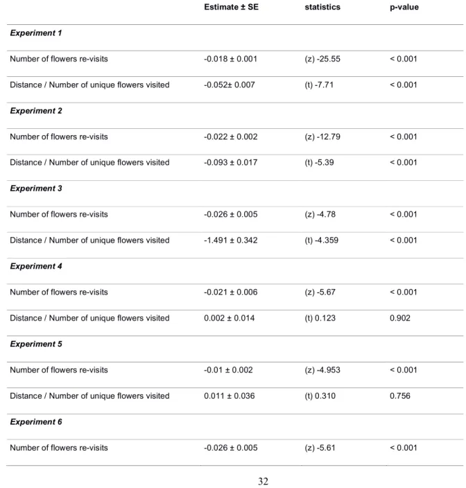
To illustrate the benefits of using the network approach relative to more conventional analyses, we 259

also calculated non-network measures used in previous studies for assessing the ability of bees to 260

develop efficient routes (Lihoreau et al., 2011; Lihoreau et al., 2012a; Lihoreau et al., 2012b; Buatois & 261

Lihoreau, 2016). For each foraging bout of each bee we calculated the number of revisits to flowers 262

and the distance travelled (assuming straight lines between flowers) divided by the number of flowers 263

visited. Both measures of route efficiency are expected to decrease with increasing network efficiency, 264

and reach a minimum in an optimal movement network. We applied a GLMM for count data to study 265

the impact of experience (foraging bout) on the number of revisits to flowers and a linear mixed effect 266

model (LMM) for the travelled distance divided by the number of flowers visited. Both models were run 267

for each experiment using individual identity as random effect. 268

269

Results

270

Local network measures 271

The average weighted betweenness centrality increased as bees accumulated foraging experience in 272

the six experiments (estimatebout = 0.066, standard error (se) = 0.004, t = 17.11, P < 0.001), indicating

273

that individuals tended to visit all flowers at a similar frequency by the end of training (Figure 4). This 274

tendency was stronger in large spatial scale arrays (estimatesmall_array = -0.067, se = 0.005, t = -13.55,

275

P < 0.001). Interestingly, in small spatial scale arrays bumblebees showed higher average weighted 276

betweenness centrality (estimatehoneybees = -1.172, se = 0.164, t = -7.15, P < 0.001) and a tendency to

277

develop optimal networks faster (estimatehoneybees = -0.020, se = 0.008, t = -2.533, P = 0.011) than

278

honeybees (Figure 4). 279

The average Kleinberg’s authority scores also increased as bees accumulated experience in 280

the six experiments (estimatebout = 0.083, se = 0.03, t = 2.781, P = 0.004), meaning that all flowers

281

became equally important in the network. For both bee species, the average authority scores were 282

9

lower in small spatial scale arrays than in large spatial scale arrays (estimatesmall_arrays = -0.446, se =

283

0.103, t = -4.334, P < 0.001). However, honeybees had larger average authority scores than 284

bumblebees in the small spatial scale arrays (estimatesmall_arrays_honeybees = 0.582, se = 0.111, t = 5.229,

285

P < 0.001) meaning that they tended to use all possible connections between flowers equally whereas 286

bumblebees only used a few. 287

The average clustering coefficient tended to decrease with time, as bees accumulated 288

foraging experience (Figure 6). Specifically, bumblebees showed a significant decrease in average 289

clustering coefficient while honeybees maintained stable values throughout the experiments 290

(estimatebout_honeybees= 0.018, se = 0.004, t = 4.185, P < 0.001). Honeybees showed completely

291

different trend at small spatial scales, by increasing their average clustering coefficient scores with 292

experience (estimatehoneybees_small_arrays = 0.407, se = 0.148, t = 2.752, P = 0.006). This again illustrates

293

the much reduced route optimisation efficiency of honeybees in comparison to bumblebees at small 294

spatial scales (Figure 6). 295

Overall, these changes in all three local network measures were more pronounced at larger 296

spatial scales, where flowers were distant from each other and from the colony nest, both for 297

bumblebees and honeybees (Figures 4, 5 and 6). 298

299

Global network measures 300

While bees initially used the 16 possible motifs to link flowers, they gradually reduced the number of 301

motifs to only use two of them by the end of training (motifs 2 and 6), a behaviour that is characteristic 302

of route optimisation (Figure 3). This tendency was less pronounced for honeybees at small spatial 303

scales (Figures 3D and 3E). Analyses of the frequency usage of each motif confirmed that honeybees 304

at small spatial scales often presented opposite tendencies than honeybees at large spatial scales or 305

bumblebees at all spatial scales (Figure 3D: motifs 3, 7, 8 and 15; Figure 3E: motifs 4, 5, 10 and 15) 306

(for detailed motifs analysis see Table S4-S9). 307

308

Other measures 309

Conventional statistics for bee movement analyses showed trends towards a general increase in 310

movement efficiency with experience. In all experiments bees decreased the number of revisits to 311

flowers as they accumulated foraging bouts (Table S10). Bees also tended to decrease their travelled 312

distance divided by the number of visited flowers, except in the case of honeybees foraging in small 313

spatial scale arrays (Table S10). 314

315

Discussion

316

Network analyses are increasingly used in behavioural and ecological research, providing a whole 317

new range of metrics to describe and model interactions between individuals and their environment 318

(Croft et al., 2008; Jeanson, 2012; Pinter-Wollman et al., 2013). In pollination ecology, this approach 319

has proved particularly powerful to describe interactions between plant and pollinator species, for 320

instance using undirected bipartite networks based on field surveys of pollinator abundance (e.g. 321

(Fontaine et al., 2006; Bascompte & Jordano, 2007; Campbell et al., 2011; Burkle et al., 2013; Coux et 322

10

al., 2016). Here we show how spatial network analyses can be developed to study the movement 323

patterns of individual bees exploiting multiple feeding locations at various spatial and temporal scales 324

in simplified experimental conditions. We argue that this approach may prove particularly helpful to 325

analyse pollinator movements in more complex and ecologically realistic experimental designs and to 326

generate new empirically testable hypotheses for pollination ecology research. 327

As illustrated above, bee movement patterns can be described in terms of local and global 328

network metrics that change predictably as individuals accumulate foraging experience. For instance, 329

in a simple situation where only one bee exploits a stable array of flowers refilled between each 330

foraging bout, both average betweenness values and average authority scores increased with time. By 331

contrast the average clustering of flowers decreased with time as bees started to develop optimal or 332

suboptimal stable movement networks. This tendency for optimisation of spatial movement networks 333

was also reflected in the dynamics of motif usage, resulting in bees increasing their usage of the only 334

two motifs representative of an optimal foraging route. Interestingly, and in accordance with previous 335

studies (e.g. Saleh & Chittka, 2007; Lihoreau et al., 2012a; Buatois & Lihoreau 2016), we found that 336

bumblebees and honeybees rarely use optimal spatial networks at small spatial scales, where the cost 337

of using a longer (suboptimal) path may be negligible. By contrast, foragers bees always used optimal 338

spatial networks at large spatial scales, suggesting that they use more complex optimisation 339

movement rules in more costly conditions. These results were confirmed with more conventional 340

statistical approaches (e.g. flower re-visits, travel efficiency), thereby validating our approach. 341

Importantly, the global network approach, based on motif analyses, brought new insights into the 342

spatial behaviour of bees. For instance the foraging patterns of honeybees were characterised by 343

frequent back and forth movements between flowers (Figure 6D - i.e. motifs 7 & 8) and 344

disproportionate usage of specific flowers or local hubs (Figure 6D – i.e. motif 4). 345

The aim of this exploratory study was to introduce spatial network analyses for characterising 346

bee movement patterns using relatively standard metrics. Further developments of this approach will 347

provide a powerful, complementary, analytical tool to conventional behavioural metrics in order to 348

inform researchers about spatial processes that are not captured by other measures. This approach 349

should focus more on global measures of path optimality (e.g. network path length, geodesic distance 350

“Wasserman & Faust, 1994”) to discriminate these different scenarios. For instance, network triads 351

give new information about specific movement routines that may be repeated within a route but that 352

are hardly detectable with current measures of sequence repeatability (Thomson et al., 1997; Ayers et 353

al., 2015). Ultimately, a major challenge for future studies will be to consider the high levels of 354

heterogeneity among flower resources that bees may face in nature, taking into account variation in 355

resource reward quantity and quality, signals, and competition among foragers in addition to spatial 356

constraints of resource locations, in order to extend our approach to field conditions. Experimentally, 357

bumblebees foraging in arrays of artificial flowers providing different nectar rewards face a trade off 358

between maximising their nectar intake rate and minimizing travel distances when developing traplines 359

(Lihoreau et al., 2011). Analyses on non-averaged local metrics could be used to capture the effect of 360

resource diversity in network formation, and bring new insights into how bees integrate memories of 361

multiple individual flowers in their spatial memory. The Kleinberg’s authority score likely informs us 362

11

about how bees use flowers as reference points relative to neighbouring flowers, perhaps to locate 363

new flowers at the beginning of route formation. The weighted clustering coefficient is a mean to 364

determine the level of connections between sub-groups flowers, a measure that should greatly vary 365

during the process of route optimisation. Other network measures, not used here, may also help 366

understand how bees change their foraging area with experience or in the face of competition (e.g. 367

modularity in Dupont et al., 2014). 368

While some of the predictions tested here may seem rather intuitive, our analysis of bumblebee and 369

honeybee movement patterns in relatively simple foraging conditions aims at illustrating how network 370

statistics could serve future research in field and semi-field conditions. Motif network analyses offer the 371

possibility to statistically compare networks to each other, either for the same individuals at different 372

stages of route formation, or between different individuals, and between different species. 373

Characterising the spatial foraging strategies of a wider range of pollinators, including wild and 374

managed species is a key challenge of pollination ecology in order to identify and compare the real 375

impact of these species on pollination services (Garibaldi et al., 2013). For instance, our preliminary 376

analysis suggests that at small spatial scales bumblebees display more efficient spatial movements 377

than honeybees. Bumblebees tended to reach a frequency of each triadic structure that would lead to 378

an optimal foraging network, whereas honeybees often showed the opposite behaviour. A possible 379

explanation is the difference of social life style between these two pollinator species. Honeybees, in 380

contrast to bumblebees, have evolved a unique food recruitment system (the waggle dance) by which 381

successful foragers communicate locational information about food resources to their nestmates upon 382

their return to the hive (Von Frisch, 1967; Dornhaus et al., 2006). These insects may thus invest less 383

in individual sampling and efficient route learning than species lacking the means to communicate 384

foraging locations, such as bumblebees (Buatois & Lihoreau, 2016). Another possibility is the 385

difference of typical foraging range between the two species. While bumblebees rarely cover more 386

than three kilometres to exploit floral resources (Osborne et al., 2008), honeybees can travel more 387

than ten kilometres within a single foraging trip (Pahl et al., 2011), suggesting that they are better 388

adapted to long flights and could start exhibiting optimisation movement patterns at larger spatial 389

scales than bumblebees. Systematic comparisons of both species across a wider range of spatial 390

scales will be needed to test these hypotheses. 391

Another key advantage of network analyses is that they allow for working on complete (raw) 392

datasets and thus reduce the risks of arbitrarily discarding important information. In the case of 393

pollinators, such approach may allow identification of specific movement patterns that occur at the 394

early stage of route learning, for instance exploration flights to locate flowers and store them in spatial 395

memory, or exploitation flights to return to familiar locations (Woodgate et al., 2016). Further 396

development of pollinator movement networks may also include detailed dynamic temporal analyses 397

of flower visitation sequences, which might reveal differential effect of the individual experience on the 398

probability to optimize the foraging route. Stochastic agent-based methods (Snijders et al., 2010) 399

recently applied to animal social networks (Boucherie et al., 2016; Pasquaretta et al., 2016), may also 400

prove useful to integrate rate of change of flower visitation sequences. New metrics could be 401

developed to estimate network efficiency in order to account for the specificity of the structure of bee 402

12

spatial movement based on individual experience. For instance, the direct integration of probability 403

values based on the spatial distances between flowers will allow for a finer calculation of local network 404

metrics which could be used to characterize the individual learning process and compare the likelihood 405

to obtain an optimal foraging route depending on the early spatial experience of the bee. Explicit 406

consideration of the nest as a specific node in the network, different from flowers, may also bring 407

useful information about bee network dynamics and efficiency. 408

For all these reasons, we believe that pollinator movement networks constitutes a highly 409

promising conceptual framework for studying plant-pollinator systems from a mechanistic point of view 410

in complement to more conventional behavioural measures. Ultimately, a comprehensive 411

understanding of bee movement patterns between plants may provide new fundamental insights into 412

pollination processes and the genetic structuralism of plant populations. The development of optimal 413

routes by individual bees between particular plants can have important and predictable effects on 414

plant reproduction and inbreeding (Ohashi & Thomson, 2009). Advances in DNA pollen analyses (see 415

Clare et al., 2013; and metabarcoding; Pornon et al., 2016) now allow identification of flower species 416

visited by individual bees during a given foraging trip. One can readily downscale the approach at an 417

intraspecific level by using pollen DNA and more variable genetic markers (e.g. microsatellite; Arif et 418

al., 2010) to identify individual plants visited by pollinators and infer patterns of pollen flow within a 419

plant population that can then be verified by paternity analyses using plant progeny genotypes for 420

these markers (Bernasconi, 2003). Coupling these approaches with existing models of bee 421

movements (Lihoreau et al., 2012b; Reynolds et al., 2013; Becher et al., 2016) will provide critical 422

information about how the foraging strategies of bees directly influence pollen transfer and plant 423

mating patterns across landscapes, and therefore a better assessment of consequences of bee 424

declines on pollination. 425

426 427

Contribution of the authors 428

ML designed and conducted the experiments; CP built and analysed the networks; CP, RJ, CA, LC 429

and ML wrote the manuscript. All authors gave final approval for publication. Authors declare no 430 competing interests. 431 432 Funding 433

CP is funded by a grant of the Federal University of Toulouse (IDEX UNITI) to CA, RJ and ML. LC is 434

supported by ERC grant SpaceRadarPollinator. ML is supported by an ANR Jeune Chercheur (ANR-435 16-CE02-0002-01). 436 437 438 439 References 440

Akaike H. (1985) Prediction and Entropy. In: Atkinson A.C., Fienberg S.E. (eds) A Celebration of 441

Statistics. Springer, New York, NY. pp. 387–410. 442

13

Arif, I.A., Khan, H.A., Shobrak, M., Al Homaidan, A.A., Al Sadoon, M., Al Farhan, A.H., et al. (2010) 443

Interpretation of electrophoretograms of seven microsatellite loci to determine the genetic diversity of 444

the Arabian Oryx. Genetics and Molecular Research, 9, 259–265. 445

Ayers, C.A., Armsworth, P. R., & Brosi, B. J. (2015). Determinism as a statistical metric for ecologically 446

important recurrent behaviors with trapline foraging as a case study. Behavioral ecology and 447

sociobiology, 69, 1395-1404. 448

Barrat, A., Barthelemy, M., Pastor-Satorras, R. & Vespignani, A. (2004) The architecture of complex 449

weighted networks. Proceedings of the National Academy of Sciences of the United States of 450

America, 101, 3747–3752. 451

Barthélemy, M. (2011) Spatial networks. Physics Reports, 499, 1–101. 452

Bascompte, J. & Jordano, P. (2007) Plant-animal mutualistic networks: The architecture of 453

biodiversity. Annual Review of Ecology, Evolution, and Systematics, 38, 567–593. 454

Becher, M.A., Grimm, V., Knapp, J., Horn, J., Twiston-Davies, G. & Osborne, J.L. (2016) BEESCOUT: 455

A model of bee scouting behaviour and a software tool for characterizing nectar/pollen landscapes for 456

BEEHAVE. Ecological Modelling, 340, 126–133. 457

Bernasconi, G. (2003) Seed paternity in flowering plants: an evolutionary perspective. Perspectives in 458

Plant Ecology, Evolution and Systematics, 6, 149–158. 459

Boucherie, P.H., Sosa, S., Pasquaretta, C. & Dufour, V. (2016) A longitudinal network analysis of 460

social dynamics in rooks corvus frugilegus: repeated group modifications do not affect social network 461

in captive rooks. Current zoology, zow083. doi: 10.1093/cz/zow083 462

Buatois, A. & Lihoreau, M. (2016) Evidence of trapline foraging in honeybees. The Journal of 463

Experimental Biology, 219, 2426–9. 464

Burkle, L.A. & Alarcón, R. (2011) The future of plant-pollinator diversity: Understanding interaction 465

networks acrosss time, space, and global change. American Journal of Botany, 98, 528–538. 466

Burkle, L.A., Marlin, J.C. & Knight, T.M. (2013) Plant-pollinator interactions over 120 years: Loss of 467

species, co-occurrence, and function. Science, 339, 1611–1615. 468

Campbell, C., Yang, S., Albert, R. & Shea, K. (2011) A network model for plant-pollinator community 469

assembly. Proceedings of the National Academy of Sciences of the United States of America, 108, 470

197–202. 471

Chittka, L., Gumbert, A. & Kunze, J. (1997) Foraging dynamics of bumble bees: correlates of 472

movements within and between plant species. Behavioral Ecology, 8, 239–249. 473

Chittka, L. & Thomson, J.D. (2001) Cognitive ecology of pollination: animal behaviour and floral 474

evolution. Cambridge University Press. New York. NY 475

Clare, E.L., Schiestl, F.P., Leitch, A. R., & Chittka, L. (2013) The promise of genomics in the study of 476

plant-pollinator interactions. Genome Biology, 14, 207. 477

Collett, M., Chittka, L. & Collett, T.S. (2013) Spatial memory in insect navigation. Current Biology, 23, 478

R789–R800. 479

Cook, W. (2012) In pursuit of the traveling salesman: mathematics at the limits of computation. 480

Princeton University Press. Princeton. New Jersey 481

Coux, C., Rader, R., Bartomeus, I. & Tylianakis, J.M. (2016) Linking species functional roles to their 482

network roles. Ecology Letters, 19, 762–770. 483

14

Crall, J.D., Gravish, N., Mountcastle, A.M. & Combes, S.A. (2015) BEEtag: a low-cost, image-based 484

tracking system for the study of animal behavior and locomotion. PloS ONE, 10, e0136487. 485

Croft, D.P., James, R. & Krause, J. (2008) Exploring animal social networks. Princeton University 486

Press. Princeton. New Jersey 487

Csardi, G. & Nepusz, T. (2006) The igraph software package for complex network research. 488

InterJournal, Complex Systems, 1695, 1–9. 489

Dorigo, M. & Gambardella, L.M. (2016) Ant-Q: A reinforcement learning approach to the traveling 490

salesman problem. In Proceedings of ML-95, Twelfth International Conference on Machine Learning. 491

Eds Morgan Kaufmann. pp. 252–260. 492

Dornhaus, A., Klügl, F., Oechslein, C., Puppe, F. & Chittka, L. (2006) Benefits of recruitment in honey 493

bees: effects of ecology and colony size in an individual-based model. Behavioral Ecology, 17, 336– 494

344. 495

Dupont, Y.L., Trøjelsgaard, K., Hagen, M., Henriksen, M. V., Olesen, J.M., Pedersen, N.M.E., et al. 496

(2014) Spatial structure of an individual-based plant-pollinator network. Oikos, 123, 1301–1310. 497

Fontaine, C., Dajoz, I., Meriguet, J. & Loreau, M. (2006) Functional diversity of plant-pollinator 498

interaction webs enhances the persistence of plant communities. PLoS Biology, 4, 0129–0135. 499

Freeman, L. (1979) Centrality in social networks conceptual clarification. Social Networks, 1, 215–239. 500

Frisch, K. Von. (1967) The dance language and orientation of bees. Harvard University press. 501

Cambridge 502

Garibaldi, L.A., Steffan-Dewenter, I., Winfree, R., Aizen, M.A., Bommarco, R., Cunningham, S.A., et al. 503

(2013) Wild pollinators enhance fruit set of crops regardless of honey bee abundance. Science, 339, 504

1608–1611. 505

Goulson, D., Nicholls, E., Botías, C. & Rotheray, E.L. (2015) Bee declines driven by combined stress 506

from parasites, pesticides, and lack of flowers. Science, 347, 1255957. 507

Heinrich, B., (1976) the foraging specializations of individual bumble-bees. Ecological Monographs, 508

46, 105-128. 509

Ings, T.C. & Chittka, L. (2008) Speed-accuracy tradeoffs and false alarms in bee responses to cryptic 510

predators. Current Biology, 18, 1520–1524. 511

Jacoby, D.M.P. & Freeman, R. (2016) Emerging network-based tools in movement ecology. Trends in 512

Ecology & Evolution, 31, 301-314. 513

Janzen, D.H. (1971) Euglossine bees as long-distance pollinators of tropical plants. Science, 171, 514

203–205. 515

Jeanson, R. (2012) Long-term dynamics in proximity networks in ants. Animal Behaviour, 83, 915– 516

923. 517

Klein, S., Cabirol A., Devaud, J.M., Barron, A.B. & Lihoreau, M. (2017) Why bees are so vulnerable to 518

environmental stressors. Trends in Ecology & Evolution, 32, 268-278. 519

Kleinberg, J. (1999) Authoritative sources in a hyperlinked environment. Journal of the ACM (JACM), 520

46, 604–632. 521

Kovanen, L., Karsai, M., Kaski, K., Kertész, J. & Saramäki, J. (2011) Temporal motifs in time-522

dependent networks. Journal of Statistical Mechanics: Theory and Experiment, 11, P11005. 523

https://doi.org/10.1088/1742-5468/2011/11/P11005 524

15 525

Lihoreau, M., Chittka, L. & Raine, N.E. (2010) Travel optimization by foraging bumblebees through 526

readjustments of traplines after discovery of new feeding locations. The American Naturalist, 176, 527

744–757. 528

Lihoreau, M., Chittka, L. & Raine, N.E. (2011) Trade-off between travel distance and prioritization of 529

high-reward sites in traplining bumblebees. Functional Ecology, 25, 1284–1292. 530

Lihoreau, M., Chittka, L., Le Comber, S.C. & Raine, N.E. (2012a) Bees do not use nearest-neighbour 531

rules for optimization of multi-location routes. Biology letters, 8, 13–6. 532

Lihoreau, M., Raine, N.E., Reynolds, A.M., Stelzer, R.J., Lim, K.S., Smith, A.D., et al. (2012b) Radar 533

tracking and motion-sensitive cameras on flowers reveal the development of pollinator multi-534

destination routes over large spatial scales. PLoS Biology, 10, 19–21. 535

Lihoreau, M., Chittka, L. & Raine, N.E. (2016) Monitoring flower visitation networks and interactions 536

between pairs of bumble bees in a large outdoor flight cage. PloS ONE, 11, e0150844. 537

Makino, T.T. & Sakai, S. (2004) Findings on spatial foraging patterns of bumblebees (Bombus ignitus) 538

from a bee-tracking experiment in a net cage. Behavioral Ecology and Sociobiology, 56, 155-163. 539

Makino, T.T. & Sakai, S. (2005) Does interaction between bumblebees (Bombus ignitus) reduce their 540

foraging area?: bee-removal experiments in a net cage. Behavioral Ecology and Sociobiology, 57, 541

617-622. 542

Makino, T.T. (2013) Longer visits on familiar plants?: testing a regular visitor’s tendency to probe more 543

flowers than occasional visitors. Naturwissenschaften, 100, 659-666. 544

Mayer, C., Adler, L., Armbruster, W., Dafni, A., Eardley, C., Huang, S., et al. (2011) Pollination ecology 545

in the 21st Century: key questions for future research. Journal of Pollination Ecology, 3, 8–23. 546

Michener, C.D. (2000) The Bees of the World. JHU Press. Baltimore 547

Milo, R., Shen-Orr, S., Itzkovitz, S., Kashtan, N., Chklovskii, D. & Alon, U. (2002) Network motifs: 548

Simple building blocks of complex networks. Science, 298, 824–827. 549

Nandi, A.K., Sumana, A. & Bhattacharya, K. (2014) Social insect colony as a biological regulatory 550

system: modelling information flow in dominance networks. Journal of The Royal Society Interface, 11, 551

20140951 552

Ohashi, K., Thomson, J.D. & D’Souza, D. (2007) Trapline foraging by bumble bees: IV. Optimization of 553

route geometry in the absence of competition. Behavioral Ecology, 18, 1–11. 554

Ohashi, K. & Thomson, J.D. (2009) Trapline foraging by pollinators: Its ontogeny, economics and 555

possible consequences for plants. Annals of Botany, 103, 1365–1378. 556

Ohashi, K., D’Souza, D. & Thomson, J.D. (2010) An automated system for tracking and identifying 557

individual nectar foragers at multiple feeders. Behavioral Ecology and Sociobiology, 64, 891–897. 558

Opsahl, T. (2009) Structure and evolution of weighted networks. University of London (Queen Mary 559

College), London, UK, pp. 104-122. Available at 560

https://toreopsahl.files.wordpress.com/2009/05/thesis_print-version_withoutappc.pdf 561

Osborne, J.L., Martin, A.P., Carreck, N.L., Swain, J.L., Knight, M.E., Goulson, D., et al. (2008) 562

Bumblebee flight distances in relation to the forage landscape. Journal of Animal Ecology, 77, 406– 563

415. 564

16

Pahl, M., Zhu, H., Tautz, J. & Zhang, S. (2011) Large scale homing in honeybees. PLoS ONE, 6, 565

e19669. 566

Pasquaretta, C., Klenschi, E., Pansanel, J., Battesti, M., Mery, F. & Sueur, C. (2016) Understanding 567

dynamics of information transmission in Drosophila melanogaster using a statistical modeling 568

framework for longitudinal network data (the RSiena package). Frontiers in psychology, 7, 539. 569

Perna, A. & Latty, T. (2014) Animal transportation networks. Journal of the Royal Society, Interface / 570

the Royal Society, 11, 20140334. 571

Pinter-Wollman, N., Hobson, E.A., Smith, J.E., Edelman, A.J., Shizuka, D., de Silva, S., et al. (2013) 572

The dynamics of animal social networks: Analytical, conceptual, and theoretical advances. Behavioral 573

Ecology 25, 242-255. 574

Polyakovskiy, S., Bonyadi, M.R., Wagner, M., Michalewicz, Z. & Neumann, F. (2014) A 575

comprehensive benchmark set and heuristics for the traveling thief problem. In Proceedings of the 576

2014 Annual Conference on Genetic and Evolutionary Computation. Eds. Christian Igel. ACM, New 577

York. NY pp. 477–484. 578

Pornon, A., Escaravage, N., Burrus, M., Holota, H., Khimoun, A., Mariette, J., et al. (2016) Using 579

metabarcoding to reveal and quantify plant-pollinator interactions. Scientific Reports, 6, 27282. 580

Pyke, G.H. & Cartar, R. V. (1992) The flight directionality of bumblebees: Do they remember where 581

they came from? Oikos, 65, 321–327. 582

Quevillon, L.E., Hanks, E.M., Bansal, S. & Hughes, D.P. (2015) Social, spatial, and temporal 583

organization in a complex insect society. Scientific reports, 5, 13393 584

Reynolds, A.M., Lihoreau, M. & Chittka, L. (2013) A simple iterative model accurately captures 585

complex trapline formation by bumblebees across spatial scales and flower arrangements. PLoS 586

Computational Biology, 9, e1002938. 587

Rigby, R.A. & Stasinopoulos, D.M. (2005) Generalized additive models for location, scale and shape. 588

Journal of the Royal Statistical Society: Series C (Applied Statistics), 54, 507-554. 589

Saleh, N. & Chittka, L. (2007) Traplining in bumblebees (Bombus impatiens): a foraging strategy’s 590

ontogeny and the importance of spatial reference memory in short-range foraging. Oecologia, 151, 591

719-730. 592

Shizuka, D. & McDonald, D.B. (2015). The network motif architecture of dominance hierarchies. 593

Journal of The Royal Society Interface, 12, 20150080. 594

Snijders, T.a.B., van de Bunt, G.G. & Steglich, C.E.G. (2010) Introduction to stochastic actor-based 595

models for network dynamics. Social Networks, 32, 44–60.Thomson, J.D. (1986) Pollen transport and 596

deposition by bumble bees in Erythronium: influences of floral nectar and bee grooming. Journal of 597

Ecology, 74, 329-341. 598

Thomson, J.D., Slatkin, M. & Thomson, B.A. (1997) Trapline foraging by bumble bees: II. Definition 599

and detection from sequence data. Behavioral Ecology, 8, 199–210. 600

Tylianakis, J.M., Tscharntke, T. & Lewis, O.T. (2007) Habitat modification alters the structure of 601

tropical host–parasitoid food webs. Nature, 445, 202-205. 602

Waser, N.M. (1986). Flower constancy: definition, cause, and measurement. The American Naturalist, 603

127, 593-603. 604

Wasserman, S. & Faust, K. (1994) Social network analysis: Methods and applications. Cambridge 605

University Press. New York. NY 606

17

Waters, J.S. & Fewell, J.H. (2012) Information processing in social insect networks. PLoS ONE, 7, 607

e40337. 608

Woodgate, J.L., Makinson, J.C., Lim, K.S., Reynolds, A.M. & Chittka, L. (2016) Life-long radar tracking 609

of bumblebees. PloS ONE, 11, e0160333. 610

18

Figure legends

Figure 1. Examples of local and global metrics calculated on a bee spatial movement network. Nodes of the network (white circles) represent flowers (F1-F6) and the colony nest (black square). Edge directions indicate individual movements between flowers and the nest. Edge thickness is proportional to the frequency of bee movements from one flower to another (i.e. edge weights). In this hypothetical network, from A to E, the forager tends to increase the number of visited flowers with experience (t0, t0 + 1, t0 + 2, t0 + n) while reducing both the number of revisits to flowers and the time needed to visit all (i.e. network optimization). Examples of local network

measures are shown (black arrows): 1) High clustering coefficient calculates the degree to which neighbours of a given node are themselves highly connected; 2) Authority score indicates the existence of highly visited nodes; 3) High betweenness centrality value counts the number of shortest paths that pass through a focal node. (F) Hypothetical network illustrating two common network motifs (red arrows) in bee movement data (motifs 3 and 6, see Figure 3).

19

Figure 2. Spatial arrangements of the artificial flowers (F1-F6) and the colony nest (black square) in the six experiments under investigation (scale is in meters). Number of bees (n) and foraging bouts (fb) are shown for each experiment. A. Experiment 1: bumblebees in the lab (Lihoreau et al., 2012a). B. Experiment 2: bumblebees in the lab (Lihoreau et al., 2011). C. Experiment 3: bumblebees in the field (Lihoreau et al., 2012b). D. Experiment 4: honeybees in the lab (Buatois & Lihoreau 2016). E. Experiment 5: honeybees in the field (Buatois & Lihoreau 2016). F. Experiment 6: honeybees in the field (Buatois & Lihoreau 2016). Spatial scales are provided for each array (i.e. SMALL or LARGE).

5 m 5 m 5 m _{5 m} 5 m

Bumblebee

Honey bee

A.

B.

C.

D.

F.

(SMALL) experiment 6(LARGE)

F1 F2 F3 F4 F1 F2 F3 F4 F1 F2 F3 F4 F5 n = 7;fb = 80 n = 10;fb = 40 n = 7;fb = 22 to 37 5 m

E.

20

Figure 3. Distribution of all possible network triadic motifs across foraging bouts. For each motif, the x-axis represents the temporally ordered foraging bouts. Red horizontal lines indicate the frequency of each motif expected in the optimal network. Best fitted lines obtained from generalized linear models using foraging bouts as predictor and frequency of motif as response variable are shown for each motif along with their standard errors (blue line and shaded grey area). Significant effects of time on the frequency of each motif are highlighted with asterisks. GLMM estimates, Z-values and P-values for each motif in each experiment are available in Tables S4-S9.

5 1 2 3 4 5 6 7 8 9 10 11 12 13 14 15 16 0 5 10 15 20 1 2 3 4 5 6 7 8 9 10 11 12 13 14 15 16 0 5 10 15 20 1 2 3 4 5 6 7 8 9 10 11 12 13 14 15 16 0 5 10 15 20 1 2 3 4 6 7 8 9 10 11 12 13 14 15 16 0 2 4 6 8 1 2 4 5 6 7 8 9 10 11 12 13 14 15 16 0 2 4 6 8 1 2 3 4 5 6 7 8 9 10 11 12 13 14 15 16 0 2 4 6 8

Bumblebee

Honey bee

Motifs occurrence Motifs occurrence Foraging bouts Foraging bouts Foraging bouts Foraging bouts Foraging bouts Foraging bouts

A.

B.

C.

D.

E.

F.

21

Relationship going in the opposite direction of the optimal network are numbered in red. Alpha level is set at 0.05. Spatial scales are provided for each graph (i.e. SMALL – a,b,d,e - or LARGE – c,f -, see also Figure 2).

22

Figure 4. Average weighted betweenness centrality values for each individual bee at each foraging bout. Black lines and grey shaded areas represent respectively the best fitted lines and their standard errors obtained from

zeroinflated mixed effect models built using foraging bouts as fixed effect and individual identity as random (see details in the methods). Spatial scales are provided for each graph (i.e. SMALL – a,b,d,e - or LARGE – c,f -; see also Figure 2). 0.1 0.2 0.3 0.4 0.5 0 20 40 60 80 Foraging bouts Betw eenness centr ality 0.0 0.1 0.2 0.3 0.4 0.5 0 10 20 30 40 Foraging bouts 0.0 0.1 0.2 0.3 0.4 0.5 0 10 20 30 Foraging bouts Betw eenness centr ality 0.0 0.1 0.2 0.3 0.4 0.5 0 10 20 30 Foraging bouts Betw eenness centr ality 0.0 0.1 0.2 0.3 0.4 0.5 0 10 20 30 Foraging bouts Betw eenness centr ality 0.1 0.2 0.3 0.4 0.5 0 10 20 30 Foraging bouts Betw eenness centr ality Bumblebees Honey bees A. experiment 1 (SMALL) B. experiment 2 (SMALL) C. experiment 3 (LARGE) D. experiment 4 (SMALL) E. experiment 5 (SMALL) F. experiment 6 (LARGE) Betw eenness centr ality

Optimal movement network Suboptimal movement network

23

Figure 5. Average authority score values for each individual bee at each foraging bout. Black lines and grey shaded areas represent respectively the best fitted lines and their standard errors obtained from zeroinflated mixed effect models built using foraging bouts as fixed effect and individual identity as random (see details in the methods). Spatial scales are provided for each graph (i.e. SMALL – a,b,d,e - or LARGE – c,f -; see also Figure 2).

Bumblebees Honey bees A. experiment 1 (SMALL) B. experiment 2 (SMALL) C. experiment 3 (LARGE) D. experiment 4 (SMALL) E. experiment 5 (SMALL) F. experiment 6 (LARGE)

Optimal movement network Suboptimal movement network

0.25 0.50 0.75 1.00 0 20 40 60 80 Foraging bouts A uthor ity score 0.25 0.50 0.75 1.00 0 10 20 30 40 Foraging bouts A uthor ity score 0.25 0.50 0.75 1.00 0 10 20 30 Foraging bouts A uthor ity score 0.2 0.4 0.6 0.8 1.0 0 10 20 30 Foraging bouts A uthor ity score 0.2 0.4 0.6 0.8 1.0 0 10 20 30 Foraging bouts A uthor ity score 0.2 0.4 0.6 0.8 1.0 0 10 20 30 Foraging bouts A uthor ity score

24

Figure 6. Average clustering coefficient values for each individual bee at each foraging bout. Black lines and grey shaded areas represent respectively the best fitted lines and their standard errors obtained from zeroinflated mixed effect models built using foraging bouts as fixed effect and individual identity as random (see details in the methods). Spatial scales are provided for each graph (i.e. SMALL – a,b,d,e - or LARGE – c,f -; see also Figure 2). Bumblebees Honey bees A. experiment 1 (SMALL) B. experiment 2 (SMALL) C. experiment 3 (LARGE) D. experiment 4 (SMALL) E. experiment 5 (SMALL) F. experiment 6 (LARGE)

Optimal movement network Suboptimal movement network

0.00 0.25 0.50 0.75 1.00 0 20 40 60 80 Foraging bouts Cluster ing coefficient 0.0 0.4 0.8 1.2 0 10 20 30 40 Foraging bouts Cluster ing coefficient 0.0 0.4 0.8 1.2 0 10 20 30 Foraging bouts Cluster ing coefficient 0.0 0.5 1.0 0 10 20 30 Foraging bouts Cluster ing coefficient 0.0 0.4 0.8 1.2 0 10 20 30 Foraging bouts Cluster ing coefficient 0.0 0.4 0.8 1.2 0 10 20 30 Foraging bouts Cluster ing coefficient

25

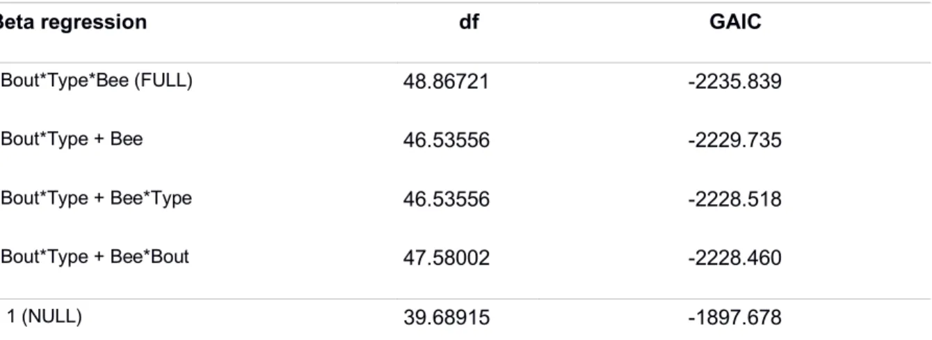
Supplementary material legends:

Table S1: Betweenness centrality model selection using the Generalised Akaike information criterion (GAIC). The three ranked best models with both FULL and NULL models are shown.

Beta regression df GAIC

~Bout*Type*Bee (FULL) 48.86721 -2235.839

~Bout*Type + Bee _{46.53556 -2229.735} ~Bout*Type + Bee*Type 46.53556 -2228.518

~Bout*Type + Bee*Bout 47.58002 -2228.460

~ 1 (NULL) 39.68915 -1897.678

Table S2: Authority model selection using the Generalised Akaike information criterion (GAIC). The three ranked best models with both FULL and NULL models are shown.

GLMM Proportional model df GAIC

~Bout*Type + Bee 25.17792 524.4065

~Bout*Type + Bee*Bout 24.60263 525.0094

~Bout*Type + Bee*Type 25.71766 527.1393

~Bout*Type*Bee (FULL) 28.58996 530.3337

~ 1 (NULL) 31.60761 538.5515

Table S3: Clustering coefficient model selection using the Generalised Akaike information criterion (GAIC). The three ranked best models with both FULL and NULL models are shown.

Beta regression df GAIC

~bout*bee+bee*type 38.44953 1829.870

~bout*type+bee*bout 39.11552 1830.968

~bout*type+bee*type+ bout*bee 39.48056 1831.826

~Bout*Type*Bee (FULL) 40.46720 1833.819

26

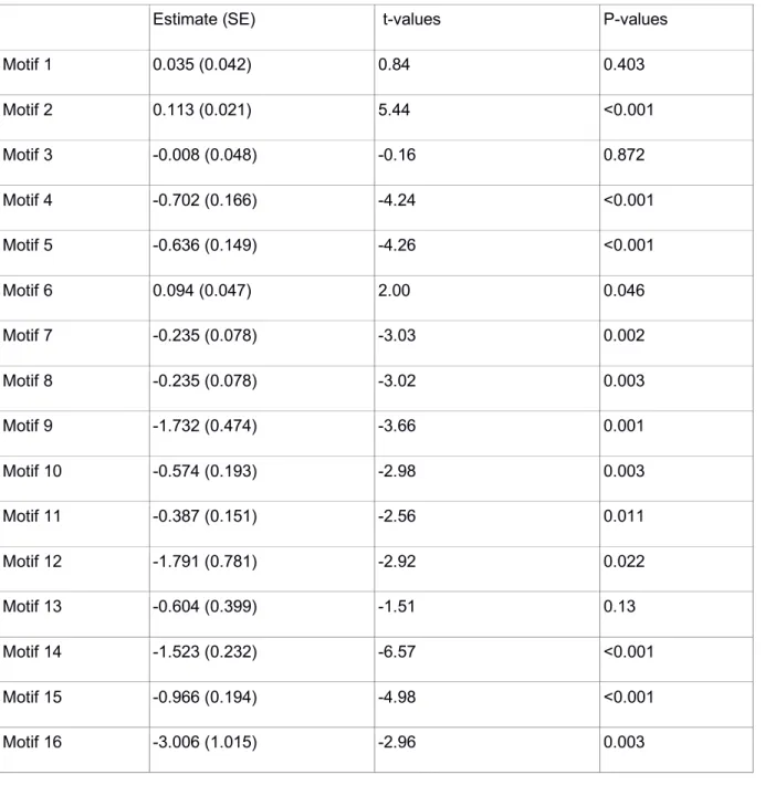
Table S4: Experiment 1 - GLMMs frequency of each network motifs and foraging bouts.

Estimate (SE) t-values P-values

Motif 1 0.035 (0.042) 0.84 0.403 Motif 2 0.113 (0.021) 5.44 <0.001 Motif 3 -0.008 (0.048) -0.16 0.872 Motif 4 -0.702 (0.166) -4.24 <0.001 Motif 5 -0.636 (0.149) -4.26 <0.001 Motif 6 0.094 (0.047) 2.00 0.046 Motif 7 -0.235 (0.078) -3.03 0.002 Motif 8 -0.235 (0.078) -3.02 0.003 Motif 9 -1.732 (0.474) -3.66 0.001 Motif 10 -0.574 (0.193) -2.98 0.003 Motif 11 -0.387 (0.151) -2.56 0.011 Motif 12 -1.791 (0.781) -2.92 0.022 Motif 13 -0.604 (0.399) -1.51 0.13 Motif 14 -1.523 (0.232) -6.57 <0.001 Motif 15 -0.966 (0.194) -4.98 <0.001 Motif 16 -3.006 (1.015) -2.96 0.003

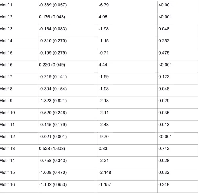
Table S5: Experiment 2 - GLMMs frequency of each network motifs and foraging bouts.

27 Motif 1 -0.389 (0.057) -6.79 <0.001 Motif 2 0.176 (0.043) 4.05 <0.001 Motif 3 -0.164 (0.083) -1.98 0.048 Motif 4 -0.310 (0.270) -1.15 0.252 Motif 5 -0.199 (0.279) -0.71 0.475 Motif 6 0.220 (0.049) 4.44 <0.001 Motif 7 -0.219 (0.141) -1.59 0.122 Motif 8 -0.304 (0.154) -1.98 0.048 Motif 9 -1.823 (0.821) -2.18 0.029 Motif 10 -0.520 (0.246) -2.11 0.035 Motif 11 -0.445 (0.179) -2.48 0.013 Motif 12 -0.021 (0.001) -9.70 <0.001 Motif 13 0.528 (1.603) 0.33 0.742 Motif 14 -0.758 (0.343) -2.21 0.028 Motif 15 -1.008 (0.470) -2.148 0.032 Motif 16 -1.102 (0.953) -1.157 0.248

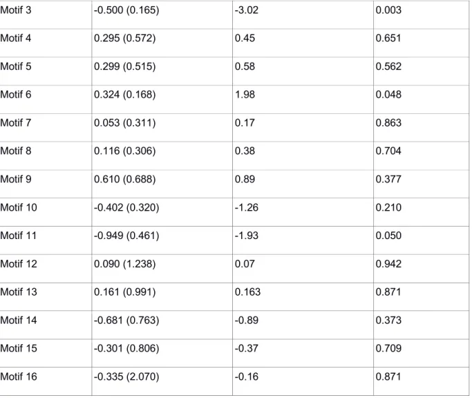
Table S6: Experiment 3 - GLMMs frequency of each network motifs and foraging bouts.

Estimate (SE) t-values P-values

Motif 1 -0.883 (0.057) -15.58 <0.001

28 Motif 3 -0.500 (0.165) -3.02 0.003 Motif 4 0.295 (0.572) 0.45 0.651 Motif 5 0.299 (0.515) 0.58 0.562 Motif 6 0.324 (0.168) 1.98 0.048 Motif 7 0.053 (0.311) 0.17 0.863 Motif 8 0.116 (0.306) 0.38 0.704 Motif 9 0.610 (0.688) 0.89 0.377 Motif 10 -0.402 (0.320) -1.26 0.210 Motif 11 -0.949 (0.461) -1.93 0.050 Motif 12 0.090 (1.238) 0.07 0.942 Motif 13 0.161 (0.991) 0.163 0.871 Motif 14 -0.681 (0.763) -0.89 0.373 Motif 15 -0.301 (0.806) -0.37 0.709 Motif 16 -0.335 (2.070) -0.16 0.871

Table S7: Experiment 4 - GLMMs frequency of each network motifs and foraging bouts.

Estimate (SE) t-values P-values

Motif 1 -0.414 (0.125) -3.31 0.002

Motif 2 -0.007 (0.098) -0.07 0.947

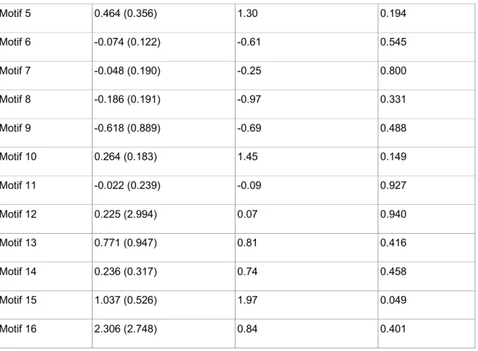
Motif 3 -0.326 (0.144) -2.27 0.024

29 Motif 5 0.464 (0.356) 1.30 0.194 Motif 6 -0.074 (0.122) -0.61 0.545 Motif 7 -0.048 (0.190) -0.25 0.800 Motif 8 -0.186 (0.191) -0.97 0.331 Motif 9 -0.618 (0.889) -0.69 0.488 Motif 10 0.264 (0.183) 1.45 0.149 Motif 11 -0.022 (0.239) -0.09 0.927 Motif 12 0.225 (2.994) 0.07 0.940 Motif 13 0.771 (0.947) 0.81 0.416 Motif 14 0.236 (0.317) 0.74 0.458 Motif 15 1.037 (0.526) 1.97 0.049 Motif 16 2.306 (2.748) 0.84 0.401

Table S8: Experiment 5 - GLMMs frequency of each network motifs and foraging bouts.

Estimate (SE) t-values P-values

Motif 1 -0.539 (0.078) -6.92 <0.001 Motif 2 -0.215 (0.083) -2.59 0.009 Motif 3 -0.114 (0.094) -1.21 0.225 Motif 4 0.277 (0.357) 0.77 0.439 Motif 5 0.045 (0.327) 0.14 0.889 Motif 6 0.112 (0.108) 1.04 0.299

30 Motif 7 0.374 (0.150) 2.49 0.013 Motif 8 0.218 (0.155) 1.39 0.163 Motif 9 0.891 (0.568) 1.57 0.118 Motif 10 0.180 (0.220) 0.82 0.413 Motif 11 -0.024 (0.166) -0.15 0.883 Motif 12 -0.024 (0.166) -0.15 0.883 Motif 13 1.195 (0.620) 1.95 0.051 Motif 14 -0.265 (0.186) -1.42 0.156 Motif 15 0.472 (0.268) 1.76 0.079 Motif 16 0.339 (0.677) 0.50 0.617

31

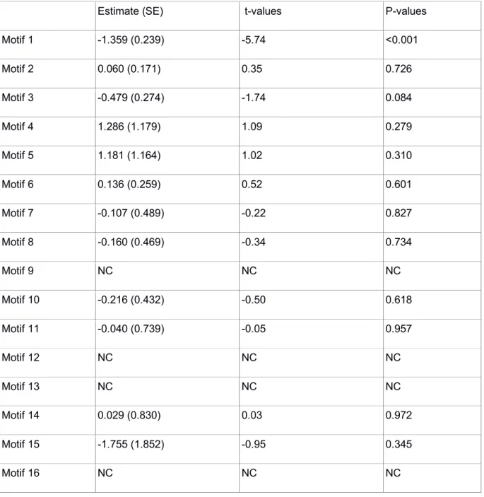
Table S9: Experiment 6 - GLMMs frequency of each network motifs and foraging bouts.

Estimate (SE) t-values P-values

Motif 1 -1.359 (0.239) -5.74 <0.001 Motif 2 0.060 (0.171) 0.35 0.726 Motif 3 -0.479 (0.274) -1.74 0.084 Motif 4 1.286 (1.179) 1.09 0.279 Motif 5 1.181 (1.164) 1.02 0.310 Motif 6 0.136 (0.259) 0.52 0.601 Motif 7 -0.107 (0.489) -0.22 0.827 Motif 8 -0.160 (0.469) -0.34 0.734 Motif 9 NC NC NC Motif 10 -0.216 (0.432) -0.50 0.618 Motif 11 -0.040 (0.739) -0.05 0.957 Motif 12 NC NC NC Motif 13 NC NC NC Motif 14 0.029 (0.830) 0.03 0.972 Motif 15 -1.755 (1.852) -0.95 0.345 Motif 16 NC NC NC