New numerical approaches for micromagnetism and Current-induced domain wall motion

(1)

HAL Id: tel-00382710

https://tel.archives-ouvertes.fr/tel-00382710

Submitted on 11 May 2009

HAL is a multi-disciplinary open access archive for the deposit and dissemination of sci-entific research documents, whether they are pub-lished or not. The documents may come from teaching and research institutions in France or abroad, or from public or private research centers.

L’archive ouverte pluridisciplinaire HAL, est destinée au dépôt et à la diffusion de documents scientifiques de niveau recherche, publiés ou non, émanant des établissements d’enseignement et de recherche français ou étrangers, des laboratoires publics ou privés.

Current-induced domain wall motion

Helga Szambolics

To cite this version:

Helga Szambolics. New numerical approaches for micromagnetism and Current-induced domain wall motion. Condensed Matter [cond-mat]. Institut National Polytechnique de Grenoble - INPG, 2008. English. �tel-00382710�

(2)

INSTITUT POLYTECHNIQUE DE GRENOBLE

N° attribué par la bibliothèque

|__|__|__|__|__|__|__|__|__|__| T H E S E

pour obtenir le grade de

DOCTEUR DE L’Institut Polytechnique de Grenoble Spécialité: Physique

préparée à l’INSTITUT NEEL

dans le cadre de l’Ecole Doctorale de Physique présentée et soutenue publiquement

par

Helga SZAMBOLICS

le 05 décembre 2008

Nouvelles formulations éléments finis pour le micromagnétisme

et

Déplacement de parois par courant polarisé en spin

DIRECTEUR DE THESE: Jean-Christophe TOUSSAINT CO-DIRECTEUR DE THESE: Liliana BUDA-PREJBEANU

JURY

M. Jean-Marc DEDULLE Président M. François ALOUGES Rapporteur M. Dafiné RAVELOSONA Rapporteur M. Jean-Christophe TOUSSAINT Directeur de thèse Mme. Liliana BUDA-PREJBEANU Co-directeur de thèse M. Nicolas VUKADINOVIC Examinateur

(3)

(4)

(5)

(6)

Remerciements

Pendant ces trois ans de thèse, j’ai eu la chance de découvrir le monde de la recherche. Je tiens tout d’abord à remercier ceux qui ont orienté mes premiers pas sur ce terrain inconnu, mes directeurs de thèse Mme Liliana Buda-Prejbeanu et M. Jean-Christophe Toussaint. Merci pour m’avoir accueillie avec tant de chaleur, pour m’avoir guidée, encouragée, conseillée pendant ces années, tout en me laissant une grande liberté. Merci pour tous ce qu’ils m’ont appris sur le plan scientifique et humain !

Mes remerciements vont aussi envers mes collègues de l’Institut Néel et du laboratoire Spintec, pour leur sympathie et leur amitié, pour les discussions intéressantes et pour la très bonne ambiance qu’ils ont su créer au sein du laboratoire.

Je voudrais remercier les membres du jury de thèse: M. François Alouges et M. Dafiné Ravelosona pour avoir accepté la responsabilité de juger mon travail de thèse en tant que rapporteurs, M. Jean-Marc Dedulle pour avoir présidé le jury de thèse et M. Nicolas Vukadinovic pour l’intérêt qu’il a porté à mon travail.

J’exprime ma gratitude envers M. Emil Burzo, Professeur à l’Université Babeş-Bolyai de Cluj-Napoca, car ma rencontre avec le micromagnétisme a été possible grâce à la collaboration franco-roumaine qu’il a initiée.

En dehors de la découverte du monde du micromagnétisme, cette expérience m’a permis de rencontrer des personnes tout à fait extraordinaires. Certains d’entre eux m’ont accompagnée pendant ces trois ans et sont devenus mes amis. Je voudrais les remercier pour m’avoir remonté le moral et pour avoir su rompre la routine des jours de travail avec les discussions partagées lors des repas ou des pauses café.

Pour leurs encouragements, leur confiance et leur soutien constants pendant mes études en France, je remercie chaudement les membres de ma famille.

(7)

Finalement, mes remerciements s’adressent plus particulièrement à mon compagnon et collègue de laboratoire Mihai Miron. Je le remercie pour sa patience et pour avoir consacré tant de temps pour faire de moi une personne beaucoup plus confiante et sûre d'elle même.

Le support financier de cette thèse a été offert par le cluster de recherche « Microélectronique, Nanosciences et Nanotechnologies » de la région Rhône-Alpes. Dans ce cadre, je voudrais remercier M. Jean-Pierre Nozières, ancien directeur du Laboratoire Spintec qui, en accordant sa confiance à notre équipe et à notre projet, s’est battu pour obtenir ce financement.

(8)

Introduction

Thanks to high-resolution fabrication and measurement techniques, one succeeds in deciphering more and more of the secrets hidden by the word “nano”. Submicron magnetic systems are now routinely fabricated based on different materials and with precisely controlled sizes and shapes [Li 2001, Jubert 2001]. Techniques like scanning tunneling microscopy and atomic (magnetic) force microscopy [Binning 1986] give access to their structural and magnetic properties. Nonetheless, even with the high performance of the available experimental techniques, certain details of the magnetization dynamics in such magnetic bodies are accessible only through micromagnetic modeling.

When it comes to magnetization dynamics, one of the topics of most interest in magnetism nowadays is the spin transfer [Slonczewski 1996]. The theoretical approaches dealing with this topic, translated the complex physical phenomenon in new terms that must be included in the dynamic Landau-Lifshitz-Gilbert equation. In this light, the purpose of the work presented here was to develop an up-to-date micromagnetic simulation tool that would make possible the treatment of systems with irregular shape, meeting certain accuracy and rapidity requirements. In other words, our goal is to find solutions of the Landau-Lifshitz-Gilbert equation, which includes the spin torque terms specific for domain wall motion, by means of micromagnetic simulations.

There are two numerical approaches widely used in numerical micromagnetism: the finite difference and the finite element approximation [Fidler 2000].

The first method is interesting because of the straightforwardness of its implementation and its rapidity, both of these qualities arising from a regular space

(11)

______________________________________________________________________________________ [García-Cervera 2003] C. J. García-Cervera, Z. Gimbutas, E. Weinan, “Accurate numerical methods for micromagnetics simulations with general geometries”, J. Comput. Phys. 184, 37 (2003).

[Braess 2001] D. Braess, “Finite elements”, 2nd ed., Cambridge University Press, Cambridge, 2001.

discretization of the magnetic body. The shortcoming of this numerical approach is that, unfortunately, any finite differences-based algorithm is intrinsically affected by the roughness of the grid at surfaces [García-Cervera 2003]. A reliable computation can be assured only for systems bounded by planar surfaces parallel to some axes of the discretization grid.

One of the solutions that would make possible to take advantage, to a certain extent, of the positive features of the finite difference approximation, while reducing its negative effects, is to correct the evaluation of the fields in the border cells. However the implementation of such corrections is not straightforward, their accuracy is not entirely guaranteed and their use can significantly increase the computation time.

Another solution, adopted by us, consists in treating the micromagnetic problem by applying the finite element approach [Braess 2001], well known for its applications to engineering problems with complex shapes. The advantage of geometry independence comes at the cost of a relatively complex mathematical apparatus. The implementation of a finite element approach is not as clear-cut as the finite difference one. Before even starting the development of a finite element software, one has to rewrite the problem to be solved (the initial partial differential equation together with the boundary conditions) under an integral form, the so-called weak formulation. One of the main issues is that this integral form is not unique.

In the present manuscript, two integral formulations for the Landau-Lifshitz-Gilbert equation were derived and implemented. The importance of choosing a correct integral form was proved based on the results obtained for several 2D test cases.

After the numerous difficulties encountered while deriving the integral form for the classical Landau-Lifshitz-Gilbert equation and implementing it, it was clear that the inclusion of the additional spin torque terms would require a large amount of time. Firstly, one has to establish a proper integral form and, secondly, this has to be implemented. Unfortunately, the first step is already a problematical task, as there is no clear criterion saying what integral form can or cannot be used. However, the aim of this work was the

(12)

______________________________________________________________________________________ [Kevorkian 1998] B. M. Kevorkian, “Contribution à la modélisation du retournement d’aimantation. Application a des systèmes magnétiques nanostructurés ou de dimensions réduites”, Ph.D. dissertation, Université Joseph Fourier, Grenoble, 1998.

development of up-to-date micromagnetic tools. To continue this work, we turned our attention to the finite difference software called GL_FFT, earlier developed in our groupby Brandusa Kevorkian [Kevorkian 1998]. In this numerical tool the classical Landau-Lifshitz-Gilbert equation is integrated. This software was tested with several occasions on various systems and with various purposes. Its accuracy and performance is therefore well established.

As mentioned previously, GL_FFT served firstly as a reference, as the results obtained with the finite element implementations had to be compared to results issued by a numerical tool that was known to be accurate. Secondly, encouraged by the growing interest in the spin torque phenomenon, we considered interesting and important to include in this software the spin torque terms, making possible the numerical study of spin-polarized current driven domain wall displacement. The so-obtained software was named WALL_ST.

One of the boiling points of this domain wall motion topic is: what kinds of materials are better suited for spintronic applications, those in which the magnetization lays in-plane or those in which an out-of-plane orientation is adopted? Before studying this question, the WALL_ST software was obviously benchmarked against analytical results (concerning out-of-plane magnetized systems) and numerical results (for the in-plane magnetized scenario). As the results were encouraging, WALL_ST was employed in studying the domain wall propagation in systems with perpendicular magnetization.

This manuscript is organized as follows:

The first chapter contains a short description of the basic notions used in micromagnetism. The main interactions occurring in a micromagnetic system are presented, together with the corresponding energy terms. Based on these the equilibrium state is defined. The chapter ends with the description of the dynamic Landau-Lifshitz-Gilbert equation.

The second chapter presents in detail the two numerical approaches used for solving the micromagnetic problem: the finite difference and the finite element method. In

(13)

the description of finite difference-based GL_FFT software, topics like the space discretization, integration scheme and the solving process of the Landau-Lifshitz-Gilbert equation are treated. In the next paragraph, first a general introduction in the finite element approximation is given. Then we derive two integral formulations for the dynamic equation. After testing the first of them on two 2D test cases, we will see what details should be modified in order to get an improved description of the magnetization dynamics. The resulting second integral formulation is benchmarked against the GL_FFT simulation tool. Finally, after determining the equilibrium configuration of a FePd thin film, small excitations are introduced in the system and the ferromagnetic resonance spectrum is determined. The results are compared to experimental data.

The last chapter concerns the magnetic domain wall dynamics in systems with perpendicular anisotropy. The chapter starts with a list of the main theoretical and experimental results concerning this topic. As our micromagnetic simulation tool adapted for the study of domain wall dynamics is derived from the GL_FFT software, in the next paragraph of this chapter only the features that had to be added or modified in order to take into account the effect of a spin-polarized current are presented. Next WALL_ST is benchmarked against other numerical approaches and analytical treatments. Then follow the results, first on ideal systems and in the last part of the chapter, trying to approach reality, several kinds of defects were introduced in the magnetic system.

(14)

I. Micromagnetic theory

A ferromagnetic body is rarely uniformly magnetized. In most of the cases, it consists of small regions with constant magnetization vector M, called magnetic domains, separated by so-called domain walls, where the orientation of the magnetization changes rapidly with the position. A relatively complete understanding of such magnetic entities can be obtained using the micromagnetic theory. William F. Brown put together the concepts previously developed by Weiss [Weiss 1907], Landau and Lifshitz [Landau-Lifshitz 1935], and created a unitary continuous theory for ferro- and ferrimagnetic systems that he named micromagnetism [Brown 1963]. Micromagnetics addresses magnetic bodies on a length scale situated between that employed by atomistic approaches and the one used in domain/magnetic microstructure analysis.

The ferro- and ferrimagnetic systems are characterized by a spontaneous magnetization MS - a net magnetic moment per unit volume, resulting from a magnetic

order even in the absence of an externally applied field. Weiss explained this collective behavior of the individual moments by the “molecular field”, whose origin, as shown by Heisenberg, lies in the exchange coupling. Due to this interaction, the magnetic moments tend to be aligned parallel to each other, and therefore the amplitude of the magnetization vector must be MS. Introducing m(r,t), the normalized magnetization vector, the first hypothesis of the micromagnetic theory becomes:

( )

,

( )

, ( , ) 1 S t M t t  ₌   =  M r m r m r (I.1)

The modulus of the magnetization is then known; its orientation however, cannot be specified based on the exchange coupling. Indeed, the sources of non-uniform magnetization distribution are forces due to coupling with the crystalline structure or due to magnetostriction, dipolar forces arising from the magnetic “charges” and due to the

(15)

presence of an external magnetic field. One can consider these forces as secondary, their effect being as a perturbation of the parallel alignment imposed by the exchange coupling, which leads to small variations of the orientation of the magnetization vector. This is the second hypothesis of the micromagnetic theory. It makes possible the substitution of the atomic moments by a continuous magnetization distribution, and all the quantities that depend on the magnetization will also be continuous functions of position and time.

Depending on the forces, external and internal, acting upon a magnetic system, different equilibrium magnetization configurations are foreseeable. The micromagnetic theory is based on the principle that a magnetic equilibrium state is reached when the total energy of the system becomes minimal. In order to have a constant MS one has to assume

conditions of constant temperature. In isothermal processes, the appropriate energy functional is the Gibbs free energy. This energy functional comports several contributions. The constituting energy terms, will be defined in the following together with the equilibrium equations. In the last part of the chapter, the equation describing the magnetization dynamics, called the Landau-Lifshitz-Gilbert equation, is introduced.

(16)

I.1.

Energy functional

The free energy of a ferromagnetic system of volume Vm and under the influence of

an external magnetic field contains four fundamental terms [Brown 1963]: the exchange, the magnetocrystalline anisotropy, the demagnetizing and the applied field energy:

tot ex anis dem app

E =E +E +E +E (I.2)

Exchange energy

This contribution arises from the short-range interaction called exchange coupling, inducing the parallel alignment of the magnetic moments. Determined by Heisenberg, the exchange interaction is the strongest coupling occuring between two neighboring spins. The most common form of the exchange Hamiltonian [Buschow 2003] is:

, 1 2 nn ex ij i j i j H J = = −

∑

S S ⋅ (I.3)

where nn stands for the nearest neighbors. The exchange integral Jij depends on the distance between the interacting

spins, its sign determining a parallel (ferromagnetic) or anti-parallel (antiferromagnetic) ordering. Jij is related to

the overlap of the magnetic orbitals of adjacent atoms and to the Pauli exclusion principle. The scalar product Si·Sj

can be easily transformed making a few basic assumptions: One can suppose that the amplitude of the spins is constant,

|Si|=|Sj|=S. Moreover, working in the framework of small deviations from the parallel

alignment of the atomic moments, the direction vectors mi, i∈{1,N}, of the spin system

can be replaced by a continuous function m=m(r) with amplitude equal to 1. Taking into account these, Si·Sj reads as:

(

)

( )

2 2 1 1 2 i j S i j i  _ _  ⋅ =  − _ − ⋅∇ _    S S r r m r (I.4)

Figure I.1: Schematic representation of the interaction between two adjacent spins Si and Sj.

Si rij Sj

ri rj

(17)

with ri the position of the spin Si (Figure I.1). Substituting (I.4) in (I.3) and considering an

isotropic exchange interaction (Jij=J), like for example in a simple cubic crystal, a

simplified form is obtained:

(

)

( )

N ₂ 2 2 , 1 2 ex i j i i j H JS JS =   = − +

∑

_ r −r ⋅∇m r _ (I.5) Based on (I.5) and on the continuity hypothesis of the micromagnetic theory, any excess resulting from the deviation from the perfectly aligned state is quantified by:

( )

(

)

2

(

( )

)

2

(

( )

)

2 m ex ex x y z V E = A _ ∇m + ∇m + ∇m _dV  

∫

r r r (I.6)

The parameter Aex (J/m) is called the exchange constant. In the simple case of a cubic

crystal, Aex is JS2/a, with a the crystalline lattice constant. Through its dependence on the

lattice constant, the exchange constant is also temperature dependent. A perfect alignment of the magnetic moments corresponds to a minimum of the exchange energy (Eex=0 J/m3).

Magnetocrystalline anisotropy energy

So far it has been established that the isotropic exchange interaction is responsible for the magnitude of the magnetization vector but gives no information about its orientation. One of the factors that can impose a certain direction of M is the electrostatic interaction between the orbitals of the electrons determining the magnetic properties and the charge distribution of the ions forming the crystal lattice. This interaction is quantified by the magnetocrystalline anisotropy energy. The name “magnetocrystalline anisotropy” already suggests the basic idea behind this concept: with respect to the arrangement of the ions in the crystal structure, certain orientations of the magnetic moments are more favorable energetically than others. These axes along which it is preferable for the magnetization to lay are called easy axes.

The magnetocrystalline energy is usually small compared to the exchange energy. Its definition depends on the symmetry of the crystalline structure [Hubert 1998]. For instance, one can define uniaxial or hexagonal magnetocrystalline anisotropy. For the simplest case of uniaxial anisotropy, the corresponding anisotropy energy has the expression:

(18)

( )

(

)

2 1 m anis anis V E =

∫

K __ − uK⋅m r __dV (I.7) Where uK is the direction of the easy axis and Kanis is the temperature dependent

anisotropy constant, expressed in J/m3.

In ultrathin layers other types of anisotropy terms (surface, interface and exchange) can also occur, and these contributions might be as important as the magnetocrystalline one.

Applied field energy

If an external field Happ is applied, the magnetization M is submitted to a torque which tends to align it parallel to the field direction. Due to the misalignment between Happ and M, a supplementary contribution has to be included in the total energy:

( )

0 m app S V E = −µ

∫

M _m r ⋅Happ r _dV (I.8) where µ0=4π·10-7 H/m is the permeability of the vacuum.

Demagnetizing energy

To minimize the last two terms the orientation of the magnetization vector is varied. However none of these contributions can be held responsible for the formation of the magnetic domains. The magnetic domain structure is organized so to avoid the formation of magnetic charges, by closing in the magnetic flux (flux-closure type domains). It is the magnetization itself that gives rise to the field imposing such a behavior. The contribution inside the magnetic material is called demagnetizing field, and the corresponding energy is named the demagnetizing energy.

Similarly with electrostatics, the sources of the demagnetizing field are the volume or the surface magnetic charges associated to the magnetization distribution inside a magnet. The magnetic charges are analogous to the electric ones, with the difference that they always appear in pairs, a magnetic charge being always balanced by one having the opposite sign.

(19)

From a magnetostatic point of view, there are three important equations connecting magnetization M, applied current density j0, magnetic induction B and magnetic field H [Jackson 1999]:

(

)

0 µ = + B H M (I.9)

and two of Maxwell’s equations:

0

∇ ⋅ =B (I.10)

∇× =H j 0 (I.11)

The magnetic field H can be decomposed in two contributions: the applied field Happ generated by the current j0 and satisfying the relations:

0 ∇× =   ∇ ⋅ =  app 0 app H j H (I.12)

and the demagnetizing field Hdem that fulfils the following conditions: 0 ∇× =   ∇⋅ = −∇⋅  dem dem H H M (I.13)

Together with the differential equations (I.10) and (I.13), boundary conditions are also imposed on the magnetic induction and the demagnetizing field:

(

)

(

_ _

)

0 0 ⋅ − = × − = int ext

dem int dem ext

n B B

n H H (I.14)

where n is the normal vector pointing always outwards, the subscript “int” corresponds to the magnetic material and “ext” to the surrounding medium. Furthermore, B is supposed to cancel at infinity. Based on the equations presented above, the demagnetizing field can be determined in two ways: using either the magnetic scalar potential approach or the magnetic vector potential approach. As from a numerical point of view it is more advantageous to use the magnetic scalar potential approach (only one unknown has to be determined, whereas for the vector potential three components are required), in the following part this method is shortly presented.

(20)

Magnetic scalar potential approach

The magnetic scalar potential approach is based on the irrotational property of the demagnetizing field. By analogy with electrostatics, it follows that this field is derived from a magnetic scalar potential Φ:

= −∇Φ

dem

H (I.15)

determined by Poisson’s equation inside the magnetic system (Figure I.2):

int ρm

∆Φ = − (I.16)

ρm=-∇⋅M being the volume density of magnetic charges

(Figure I.2). In the surrounding region, Φ is governed by the Laplace equation:

ext 0

∆Φ = (I.17)

The continuity conditions (I.14) can be turned into passage conditions for Φ:

( )

int ext int ext , , m m m S S σ _Φ _{= Φ} _∈  ∂ Φ ∂ Φ  − = − ∈  _∂ _∂  r r r r r r r n n (I.18) m

σ =M n being the surface density of the magnetic charges (Figure I.2) and S⋅ m represents

the magnetic surface. Finally a condition requiring the cancellation of the scalar potential at infinity is applied [Brown 1963, Jackson 1999].

The Green function formalism can be applied to determine the potential Φ. The Green functions associated with Poisson’s equation for the 2D and 3D case are:

( )

2 3 1 : , ln 2 1 : , 4 G G π π ′ = − − ′ ′ = _′ − 2D r r r r 3D r r r r (I.19)

The potential Φ is then given the following integral formulas:

Figure I.2: Magnetic surface and volume charges.

n σ_m=M·n V_m M ρ_m=-∇·M S_m n σ_m=M·n V_m M ρ_m=-∇·M S_m

(21)

( )

1 1 2 : ln ln 2 2 1 1 3 : 4 4 m m m m m m S m m V S D dS d l D dV dS ρ σ π π ρ σ π π Γ ′ ′ ′ ′ ′ ′ Φ = − − − − ′ ′ ′ ′ Φ = + ′ ′ − −

∫

r r r r r r r r r r r r r r (I.20)

Equations (I.20) can be rewritten in a more compact form:

( )

(

) ( )

(

) ( )

[

m

]( ) [

]( )

m m m V S m m G dV G dS G G ρ σ ρ σ ′ ′ ′ ′ ′ ′ Φ = − + − = ∗ + ∗

∫

r r r r r r r r r (I.21)

Here G∗ρm and G∗σm are the convolution products between the Green function and the

volume and surface density of the magnetic charges. Knowing the scalar potential, its gradient - the demagnetizing field - is easily determined:

( )

(

) ( )

(

) ( )

[

m

]( ) [

]( )

m m m V S m m G dV G dS G G ρ σ ρ σ ′ ′ ′ ′ ′ ′ = − ∇ − − ∇ − = − ∇ ∗ − ∇ ∗

∫

dem H r r r r r r r r r (I.22)

Before continuing, it is important to note that the first three interactions: exchange, magnetocrystalline anisotropy and Zeeman coupling are acting on a short range. The demagnetizing field depends on the magnetization distribution in the whole volume of the sample. In computational micromagnetics the calculation of this field is the most problematic one, especially its cancellation at infinity posing many difficulties.

Once the demagnetizing field calculated, the resulting energy Edemis defined in a

similar way with the applied energy:

( )

0 1 2 m dem S V E = − µ M

∫

m r ⋅H_dem r dV (I.23) This energy is minimal if the density of magnetic charges is the smallest possible. For example, the demagnetizing energy of a uniformly magnetized parallelepiped sample (shown in Figure I.3 a) can be reduced dividing the magnetic body into anti-parallel magnetized domains (Figure I.3 b and c). However, even though the domain formation is benefic from magnetostatic point of view, it is in conflict with the exchange interaction, as in the walls separating the domains the magnetization orientation varies rapidly. A stable

(22)

domain structure is therefore based on the equilibrium between the energy contributions present in the magnetic system.

Figure I.3: The magnetization and the magnetic poles in a rectangular body. a) corresponds to uniform magnetization, while b), c) depict domain structures.

(23)

I.2.

Equilibrium state

Assembling the energy terms derived previously, the total energy in reduced units (m=M(r)/MS) is:

( )

(

( )

)

( )

(

( )

)

2 2 0 0 1 1 2 m m m m tot ex anis V V S S V V E A dV K dV M dV M dV µ µ     = _∇ _ + __ − ⋅ __     − _ ⋅ _ − _ ⋅ _

∫

K app dem m m r u m r m r H r m r H m r (I.24)

for the simplest case of a uniaxial material. The terms presented here are the basic ones. Eventually, supplementary contributions arising from magnetostriction, surface and shape anisotropies, RKKY coupling have to be added.

The aim of micromagnetism is to find a distribution of magnetic moments:

( )

{

V_m, 1

}

= ∈ =

m m r r m (I.25)

that minimizes the free energy functional (I.24). Such an equilibrium magnetization distribution satisfies two equilibrium conditions:

( )

2 δ 0 δ 0 tot tot E E  ₌   >  m m (I.26)

derived from variational principles [Brown 1963, Miltat 1994]. The minimization process has to take into account the constraint of constant magnetization magnitude.

Supposing that the magnetization m is varied by a small amount: m→m+δm. The change in the total energy is then δEtot=Etot(m+δm)-Etot(m).

The variation of the exchange energy term can be determined knowing that, for a scalar λ and a vector v one has δ(∇λ)2=2∇λ·∇(δλ) and ∇·(λv)=∇λ·v+λ∇·v, and therefore

δEex is: δ 2 m ex ex x x y y z z V E =

∫

A _∇ ⋅∇m δm + ∇ ⋅∇m δm + ∇ ⋅∇m δm _dV (I.27) Then replacing

(

)

x x x x x x m δm δm m δm m ∇ ⋅∇ = ∇⋅ ∇ − ∆ (I.28)

(24)

and using the Gauss (divergence) theorem the exchange term is transformed into the sum of two integrals: one covering the magnetic volume and the second over the surface delimiting it:

(

)

2 2 2 m m m ex x x ex x x ex x x V S V A ∇ ⋅∇m δm dV = A δm ∇ ⋅m dS− A δm ∆m dV

∫

n

∫

(I.29)

Finally δEex reads as:

(

)

δ 2 δ 2 δ m m ex ex ex S V E =

∫

A m⋅ ∇ ⋅m n dS−

∫

A m⋅∆mdV (I.30)

The variation of the next two terms poses no problems:

(

)(

)

δ 2 δ m anis anis V E = −

∫

K u_K⋅m u_K⋅ m dV (I.31) 0 δ δ m app S V E = −

∫

µ M m H⋅ appdV (I.32) Finally keeping in mind that: δ δ

m m

V V

dV dV

⋅ = ⋅

∫

m Hdem

∫

m Hdem , the demagnetizing term is

easily derived:

( )

0 δ δ m dem S V E = −

∫

µ M m H⋅ _dem m dV (I.33) Putting together the components, the first variation of the total energy δEtot reads as:

(

)

( )

0 0 0 δ 2 δ 2 2 δ m m tot ex S ex anis S S S V E A dS A K M dV M M µ µ µ ∂ = ⋅ ∂   − ⋅ − ∆ + ⋅ + +   

∫

K K app dem m m n m m u m u H H m (I.34)

To obtain the equilibrium condition, both the surface and volume integrals are set to 0. Using the constraint on the magnetization |m|2=1, δm is δm=δθθθθ××××m, with δθθθθ an

infinitesimal rotation of the magnetization. The scalar product in the surface integral becomes then: 2 δ 2 δ m m ex ex S S A ⋅∂ dS= A _ ×∂ _⋅ dS ∂  ∂ 

∫

m m

∫

m m θ n n (I.35)

(25)

0 ∂ =

∂ m

n (I.36)

valid on the magnetic surface Sm. In the volume integral, noting:

(

)

( )

0 0 2 ex 2 anis S S A K M M µ µ = − ∆ + ⋅ + +

eff K K app dem

H m u m u H H m (I.37)

the effective field, the second equilibrium condition - the torque condition - is obtained: 0

× eff =

m H (I.38)

The effective field is proportional to the variational derivative of the total energy density:

0 δ 1 δ tot S M ε µ = − eff H m (I.39)

Because of the constraint on the magnetization amplitude (I.1) the field component along

m plays no role.

Conditions (I.36) and (I.38) were deduced by Brown [Brown 1963], and therefore are called the Brown equations. Their solution specifies the equilibrium state. The first one is a Neumann boundary condition, which forces the magnetization to be stationary near the free surface Sm. The second equation states that for a magnetization distribution to be at

(26)

I.3.

The Landau-Lifshitz-Gilbert equation

The Brown equations (I.36) and (I.38) are enough to define the equilibrium state of a magnetic system, but they do not specify how the system reaches this state. The magnetization dynamics can be accessed through the Landau-Lifshitz-Gilbert equation. The starting point in deducing this equation is:

0 t γ µ ∂ = − × ∂ eff M M H (I.40)

describing the magnetization’s gyrotropic reaction in the presence of the field Heff. γ is the gyromagnetic ratio of the free electron (1.7608592⋅1011 s-1T-1). From (I.40) the torque from the field Heff induces a rotation of M, with an angular velocity ω=γ µ0Heff. In this

precessional motion, the modulus and the component of M along the field Heff do not change. Consequently the energy of the system is constant.

The second Brown condition imposes zero torque from the effective field on M at equilibrium. Equation (I.40) in its present form cannot describe the dissipation process resulting in a parallel alignment of Heff and M. To include the relaxation of M towards the equilibrium state, Gilbert added to the effective field a supplementary contribution,

0 α S M t γµ ∂ − ∂ M

, derived based on a Rayleigh dissipation functional approach [Gilbert 2004]. The resulting dynamic equation read as:

(

)

0 α S γµ t M t ∂  ∂  = − × +  ×  ∂ eff  ∂  M M M H M (I.41)

This equation is called the Gilbert or Landau-Lifshitz-Gilbert (LLG hereafter) equation and

α is the dimensionless damping parameter. According to this equation, the magnetization

turns around the effective field having a damped movement (Figure I.4 b). Without damping the precession of the magnetization would go on endlessly (Figure I.4 a). The damping term controls the extent of this precession: the smaller the value of α - the longer it takes for the system to arrive at equilibrium. The Gilbert form of the dynamic equation can be easily transformed [Mallinson 1987] into the previously determined Landau-Lifshitz form [Landau-Landau-Lifshitz 1935]:

(

2

)

(

)

(

)

0 0 α 1 α S γ γ µ µ t M ∂ _ _ + _∂ = − × eff −  × × eff  M M H M M H (I.42)

(27)

Figure I.4: a) Precession of the magnetization vector M around the field Heff without damping (α=0) and damped motion (α>0).

In a relaxation process, in the presence of a constant applied field, the total energy of a magnetic system can only decrease, the energy dissipation rate being:

0 . m tot V dE dV dt µ t ∂ = − ⋅ ∂

∫

eff M H (I.43)

Multiplying the LLG equation, by Heff and, respectively by ∂M/∂t results in:

(

)

(

)

2 0 α 1 and S t M t t γµ t ∂ ∂ ∂ ∂  ⋅ _∂ = − _∂ ⋅ × _∂ ⋅ × = −  _∂   

eff eff eff

M M M M

H M H M H (I.44)

Combining these relationships and then introducing the result in (I.43), the rate of change of the system’s total energy is:

2 α m tot S V dE dV dt γM t ∂   = −  _∂   

∫

M (I.45)

This is a very important property of the LLG equation as it guarantees a proper evolution towards the equilibrium state corresponding to the minimum of the total energy. Setting the damping parameter to 0, the energy of the system is preserved just as expected in the case of a Larmor precession of the magnetization around the effective field.

The form (I.41) of the dynamic equation is suitable for describing the evolution of a micromagnetic system when being under the influence of an external field. However, since the first evidence of the effect of an electric current on the magnetization, this phenomenon attracted more and more interest. In order to describe this new kind of interaction, the LLG

(28)

equation has to be adapted. The numerous theoretical showed that introducing in LLG two new torques an appropriate description of this phenomenon is obtained. Obviously, the list of physical phenomena that can be coupled with micromagnetic studies does not stop here. For example, a very interesting and absolutely necessary step in understanding the behavior of a magnetic body is the study of thermal effects.

(29)

I.4.

Towards numerical micromagnetism

The above presented micromagnetic equations (the Brown and the LLG equations) are nonlinear and non-local equations. Nonlinearities arise because of the constraint |m|2=1 and also if higher order components of the magnetocrystalline anisotropy energy are taken into account. The non-local character has its source in the definition of the demagnetizing field. All these make the micromagnetic equations difficult to solve. Analytical solutions are known for only a few simple cases, none of them including non-uniform magnetization distributions. For example, nucleation processes have been described in [Brown 1957, Frei 1957, Aharoni 1963, Eisenstein 1976, Ramesh 1988], whereas in [Stoner-Wohlfarth 1948, Kikuchi 1956, Albuquerque 2001] the macrospin approximation was employed. In most of the cases solutions are sought numerically.

From a numerical point of view, if one is interested in determining only the equilibrium state of a certain magnetic body, putting aside its dynamic behavior, one proceeds to the minimization of the total energy. For example, in [LaBonte 1969, Jakubovics 1991, Trouilloud 1987] iterative methods are used. Another possibility - giving information also about the relaxation process - consists in solving the LLG equations. It is important to note that in theoretical and numerical calculations the Gilbert damping parameter is considered to have a constant value over the sample, although there are no experimental proofs for this assumption. It is almost certain that α depends in an undetermined (and most likely non-linear) fashion on the magnetization distribution. From ferromagnetic resonance experiences and domain wall velocity measurements it has been determined that α takes values in the interval [10-4, 10-1]. For dynamic simulations, realistic values for the damping parameter have to be used, whereas to get the same outcome as from energy minimization, one can solve the LLG equations using high values of the damping parameter (over-damped regime), for example 1 or even higher.

An important remark has to be made concerning numerical techniques. These methods are based on splitting up the magnetic system into small discretization cells, the micromagnetic equations being solved for each of these discretization elements. The choice discretization elements’ size is very important, as it influences very much the accuracy of the result. The correct value is selected based on a physical criterion. This

(30)

selection rule was established based on the hypothesis that, in micromagnetism the exchange interaction is considered to be the leading one, the other interactions being viewed as perturbations. Therefore, when choosing the space step one has to take into account the extent over which the second order interactions perturb the equilibrium that would be imposed by the exchange field. There are two characteristic lengths that serve as reference [Hubert 1998]: the exchange length (lex) - quantifying the competition between

the exchange and magnetostatic interaction - and the Bloch length (lB) - the measure of the

competition between exchange and magnetocrystalline interaction:

2 0 2 and ex ex ex B S anis A A l l M K µ = = (I.46)

Making use of these two quantities, a rule of thumb was established: in micromagnetic simulations the maximum discretization element must be smaller than the minimum of these two characteristic lengths.

(31)

References

[Aharoni 1963] A. Aharoni, “Complete eigenvalue spectrum for the nucleation in a

ferromagnetic prolate spheroid”, Phys. Rev. 131, 1478 (1963).

[Albuquerque 2001] G. Albuquerque, J. Miltat, A. Thiaville, “Self-consistency based

control scheme for magnetization dynamics”, J. Appl. Phys. 89, 6791 (2001).

[Brown 1963] W. F. Brown, Jr., “Micromagnetics”, Intersience Publishers, J. Wiley and

Sons, New York, 1963.

[Brown 1957] W. F. Brown, Jr., “Criterion for uniform micromagnetization”, Phys. Rev.

105, 1479 (1957).

[Buschow 2003] K. H. J. Buschow, F. R. de Boer, “Physics of magnetism and magnetic

materials”, Kluwer Academic/Plenum Publishers, New York, 2003.

[Gilbert 2004] T. L. Gilbert, Armour Research Report (1956). T. L. Gilbert, “A

phenomenological theory of damping in ferromagnetic materials”, IEEE Trans. Magn. 40, 3443 (2004).

[Hubert 1998] A. Hubert, R. Schafer, “Magnetic domains”, Springer, New York, 1998. [Jackson 1999] J. D. Jackson, “Classical electrodynamics”, 3rd ed., Wiley, New York,

1999.

[Jakubovics 1991] J. P. Jakubovics, “Interaction of Bloch-wall pairs in thin ferromagnetic

films”, J. Appl. Phys. 69, 4029 (1991).

[Eisenstein 1976] I. Eisenstein, A. Aharoni, “Magnetization curling in a sphere”, J. Appl.

Phys. 47, 321 (1976).

[Frei 1957] E. H. Frei, S. Shtrikman, D. Treves, “Critical size and nucleation field of ideal

ferromagnetic particles”, Phys. Rev. 106, 446 (1957).

[Kikuchi 1956] R. Kikuchi, “On the minimum of magnetization reversal time”, J. Appl.

(32)

[LaBonte 1969] A. E. LaBonte, “Two-dimensional Bloch-type domain walls in ferromagnetic films”, J. Appl. Phys. 40, 2450 (1969).

[Landau-Lifshitz 1935] L. D. Landau, E. M. Lifshitz, “On the theory of the dispersion of

magnetic permeability in ferromagnetic bodies”, Phys. Z. Sowjet. 8, 153 (1935).

[Mallinson 1987] J. Mallinson, “On the damped gyromagnetic precession”, IEEE Trans.

Magn. 23, 2003 (1987).

[Miltat 1994] J. Miltat, “Domains and domains walls in soft magnetic materials, mostly”,

in Applied Magnetism, NATO ASI Series, Dordrecht: Kluwer, 221, 1994.

[Ramesh 1988] M. Ramesh, P. E. Wigen, “Ferromagnetic resonance of parallel stripe

domains-domain walls system”, J. Magn. Magn. Mat. 74, 123 (1988).

[Stoner-Wohlfarth] E. C. Stoner, E. P. Wolfahrt, “A mechanism of magnetic hysteresis in

heterogeneous alloys”, Phil. Trans. Roy. Soc. A240, 599 (1948).

[Trouilloud 1987] P. Trouilloud, J. Miltat, “Néel lines in ferrimagnetic garnet epilayers

with orthorhombic anisotropy and canted magnetization”, J. Magn. Magn. Mat. 66, 194 (1987).

[Weiss 1907] P. Weiss, “L’hypothèse du champ moléculaire et la propriété

(33)

(34)

II. Numerical micromagnetism

In the present work we are interested in solving the Landau-Lifshitz-Gilbert (LLG) partial differential equation (PDE) describing magnetization dynamics. The complexity of the LLG equation limited the number of analytical solutions, the tendency being to use numerical methods to determine approximate solutions.

There are two widely used methods: the finite difference (FD) approximation and the finite element (FE) approximation [Fidler 2000]. The FD approximation is widespread because it is easy to implement and fast [Schabes 1988, Nakatani 1989, Zhu 1989, Scheinfein 1991, Berkov 1993, Kevorkian 1998, Buda 2001, OOMMF-site] due to the possibility of computing the demagnetizing field using the Fast Fourier transforms [Masuripur 1988, FFTW-site]. The FE method is a very effective numerical tool, especially in engineering problems involving complex geometries. In micromagnetism it is less used [Fredkin 1987, Bagnérés 1991, Schrefl 1999, Fidler 2000] than the FD method, mostly because of the complex mathematical apparatus [Braess 2001] that it is founded on. The FD method solves a discrete form of the LLG equation, while in the case of the FE approximation an integral formulation is associated problem. In the first method the system is space-discretized by repetition of some regular-shaped mesh cell. The periodic discretization makes possible the replacement of the derivatives occurring in the LLG equation with expressions derived from a Taylor expansion. The method is therefore very easy to implement, but the accuracy of the solution can be affected if complex boundaries delimitate the domain [García-Cervera 2003]. The FE approximation uses an irregular discretization. Due to this, the theory behind the FE is much more complicated than the basis of the FD approximation, but the method is not restricted with respect to the geometry shape.

(35)

The present chapter is dedicated to the presentation of the two numerical methods: 1. The FD-based GL_FFT micromagnetic code, developed by Brandusa Kevorkian at

the Néel Institute in 1998 under the supervision of JC Toussaint [Kevorkian 1998], is shortly presented in the first part.

2. Then a description of the FE method is given, followed by a first FE approach developed for the LLG equation, presented together with the results obtained for two test cases. The FE results are always compared with those obtained by the GL_FFT software. In the last part of the chapter, the details and results obtained with a second FE approach are presented.

(36)

II.1.

The finite difference method

In this part, the space discretization and the relationships that determine the effective field in the FD-based GL_FFT micromagnetic software are given.

The first step in numerical calculations is to divide the magnetic system in small cells, procedure called space-discretization or meshing. The type of cells used is very important as it has great influence on the manner in which the equation is solved. In the case of the FD approach, the simulated systems are divided into regular discretization units (cubic, hexagonal, orthorhombic).

The space discretization in a bi-dimensional system contains Nx cells along the Ox direction and Ny cells along the Oy direction. The mesh cells are prisms with rectangular cross section, covering the surface δxδy (infinite along the Oz direction). For the 3D systems, the mesh consists of Nx×Ny×Nz. orthorhombic cells having each the volume

δxδyδz. A 2D and a 3D example of meshing is shown in Figure II.1:

Figure II.1: 2D and 3D finite difference discretization The evaluation of the magnetization is done in the centre of each cell:

x y z 1 1 1 δ δ δ 2 2 2 i j k x = −i  y =j−  z =k−        (II.1)

δ

x

δ

y

δ

z

→ ∞

_

x

y

z

y

x

δ

x

δ

y

δ

z

(37)

where i∈{1, …, Nx}, j∈{1, …, Ny} and k∈{1, …, Nz}. Based on this space-discretization, the vector field m(r), r∈Vm, solution of the LLG equation is in fact the magnetization

distribution {m(i,j,k)} satisfying in each mesh node |m(i,j,k)|2=1.

To find the magnetic equilibrium state, one has to evaluate the field and energy terms. The estimation of the magnetocrystalline anisotropy and the applied field energy, which are simple, local terms, is straightforward. On the other hand, the exchange field requires the estimation of the second-order derivatives of

the magnetization and the demagnetizing field is also requires a special treatment.

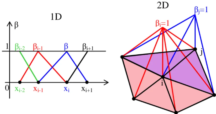
To calculate the first and second order magnetization derivatives the GL_FFT software uses the centered differences approximation, derived based on the Taylor expansion of the magnetization. For example, in a 2D case, using the grid in Figure II.2, the Taylor expansion of the magnetization gives:

(

)

( )

(

)

( )

2 2 3 x x 2 x 2 2 3 x x 2 x 1 1 δ , δ , δ 2 1 1 δ , δ , δ 2 i , j i, j i j i j O x x i , j i, j i j i j O x x ∂ ∂ + = + + + ∂ ∂ ∂ ∂ − = − + + ∂ ∂ m m m m m m m m (II.2)

The first and second order derivatives, and also the Laplacian of the magnetization can now be evaluated:

( )

(

)

(

)

( )

(

)

( )

(

)

(

)

( )

(

)

(

)

( )

(

)

x 2 2 2 x 2 2 x y 1 1, 2δ 1 2 1 δ 1 2 1 1 2 1 ∆ δ δ i , j i j i, j x i , j i, j i , j i, j x i , j i, j i , j i, j i, j i, j + − − ∂ _≅ ∂ + − + − ∂ _≅ ∂ + − + − + − + − ≅ + m m m m m m m m m m m m m m (II.3)

These relationships are applicable to the nodes situated inside the magnetic volume. For the points situated on the surface one has to make sure that the first Brown equation (see equation (I.36)), assuring the stationarity of the magnetization is respected.

(38)

Bearing these in mind, we proceed to the definition of each discrete energy and field for a bi-dimensional case.

The exchange energy

Replacing the Laplacian of the magnetization with the formula derived from the Taylor expansion the exchange field is:

(

)

( )

(

)

(

)

( )

(

)

2 2 0 x y 1 2 1 1 2 1 2 ( , ) δ δ ex S i , j i, j i , j i, j i, j i, j A i j µ M  ₊ ₋ ₊ ₋ _{+ −} ₊ ₋  =  +      ex m m m m m m H (II.4) In addition, the exchange energy is:

(

)

(

)

2

(

)

(

)

2 x y 2 2 , x,y,z x y δ δ 1 1 1, 1, , 1 , 1 4 δ δ ex ex l l l l i j l A E m i j m i j m i j m i j =     =

∑ ∑

_ + − − _ + _ + − − _ (II.5) with i∈{1, …, Nx}, j∈{1, …, Ny}.

The magnetocrystalline anisotropy contribution

In the case of uniaxial symmetry, the anisotropy field and the anisotropy energy can be written as:

( )

0 2 , anis , , , ij S K i j i j i j i j M µ   =  ⋅  anis K K H m u u (II.6)

( )

{

2

}

( )

x y , 1 , , δ δ anis anis i j E =

∑

K −_m i j ⋅uK i j _ (II.7) with i∈{1, …, Nx} and j∈{1, …, Ny}.

The applied field energy

After the discretization of the simulated system, the applied field energy takes the discrete form:

( )

0 x y , , , δ δ app S i j E = −µ M

∑

_m i j ⋅Happ i j _ (II.8) where i∈{1, …, Nx}, j∈{1, …, Ny}.

(39)

The demagnetizing term

The long-range character of the magnetostatic interaction makes the evaluation of the associated field the most complicated and time consuming one. However, quite unexpectedly, using the FD approach, this issue can be solved quite easily, namely via the Fast Fourier transforms.

The demagnetizing field is the convolution product of the magnetic charge density functions and the gradient of the Green function (see equation (I.22)). The theorem of the convolution gives a helping hand: according to this theorem, the Fourier transform (FT) of the convolution product between two functions, f and g, is equal to the ordinary product between their individual FTs:

(

)

( )

FT f ⊗g =FT f FT g (II.9)

Using this property, the demagnetizing field evaluation may be optimized by using the following steps:

1. The FT of ∇G is calculated.

2. The magnetic charge distributions are estimated from the magnetization distribution using (II.10), and then, their FTs are calculated.

( )

(

)

(

)

(

)

(

)

( )

x y , , , , 1 , 1 1, 1, 2δ 2δ , , y x m y y x x m surf m m i j i j i j x y m i j m i j m i j m i j i j i j ρ σ ∂ _∂  = − +  ∂ ∂   + − − + − − ≅ − − =m ⋅n (II.10)

3. Some ordinary operations are done in the inverse space and finally, the demagnetizing field is estimated by applying the inverse Fourier transform (FT-1):

( )

1 m m FT− FT G FT ρ FT G FT σ  = _ ∇ + ∇ _ dem H (II.11)

As the FD method solves a discrete form of the LLG equation, further optimization can be achieved passing from the continuous FT to its discrete form. The discrete form of the algorithm is called Fast Fourier transform (FFT) and has the advantage that it reduces

(40)

the number of operations [FFTW-site]. Another advantage of this method is that the FT of the ∇G is computed only one time at the beginning of the simulation [Kevorkian 1998].

Introducing these in the formula for the demagnetizing energy density one finds:

( )

0 x y , 1 , , δ δ 2 dem S i j E = − µ M

∑

_m i j ⋅H_dem i j _ (II.12)

The Landau-Lifshitz-Gilbert equation

The GL_FFT software solves the non-linear LLG equation (I.42). The time integration schemes used for this equation are various: from forward and backward Euler [Nakatani 1989], to Crank-Nicholson [Albuquerque 2001] and to fourth order Runge-Kutta schemes [Ferre 1995, Lopez 1999].

The scheme of integration used in the present FD approach is an explicit method, preserving unconditionally constant the amplitude of the magnetization vector. This scheme was derived replacing t with 0

2

1 α t

µ γ

τ =

+ and noting H(τ)=Heff(τ)+αm(τ)×Heff(τ). The dynamic equation becomes then:

( ) ( )

τ τ τ ∂ = − × ∂ m m H (II.13)

For sufficiently small time steps, the variation of H is also very small, so that H can be considered constant. Then, an exact solution of (II.13) can be found, that is in reality the analytical solution of the equation (I.42) without damping.

The series expansion of the magnetization m(t+δt) as a function of m(t) is first written:

(

)

( )

₍

( )

₎

( )

_{( )}

1 2 1 ₂ ₁ 2 ₂ 2 1 2 0 1 ! 2 1 ! 2 ! n _n n n p _p p _p p p p p t d t t t n dt t d t d t p dt p dt δ δ δ δ ∞ = + ₊ ∞ ∞ + = = + = + = = + + +

∑

m m m m m m (II.14)

(41)

( )

2 2 1 1 2 2 2 2 2 1 2 2 1 n n n n n n n d d d H H dt dt dt d d H dt dt − − + + = − = − × = − m m m H m m (II.15)

and the Taylor expansion of the magnetization m(t+δt) takes the form:

(

)

( )

₍

( )

2

_{) ( )}

1 2

( )

_{( ) ( )}

2 1 2 2 0 1 1 1 2 1 ! 2 ! p p p p p p p p t d t d t t t H H p dt p dt δ δ δ + ∞ ∞ ₋ − = = + = + − + − × +

∑

m

∑

m m m H (II.16)

Finally the following explicit integration scheme is obtained:

(

)

( ) (

)

(

)

(

( )

)

(

)

(

)

( )

2 sin cos 1 cos H t t t t H t t H t H t H δ δ δ δ + = + × + ⋅ + − m m H m m H H (II.17)

In the case of a constant field, the time integration using this scheme is exact [Kevorkian 1998].

The stability analysis permitted to establish a critical time step related to the space discretization (valid for 2D simulations):

1 0 2 2 2 x y 1 1 2α 8 δ δ α 1 S ex M A µ δτ −   = _ + _ +   (II.18)

At equilibrium the torque on the magnetization should be 0 in each discretization cell. From a numerical point of view, the 0-torque requirement is replaced by a more suitable one, namely the equilibrium state is considered to be reached, when the maximum of (m×Heff)/MS is smaller then 10-6 rad [Kevorkian 1998].

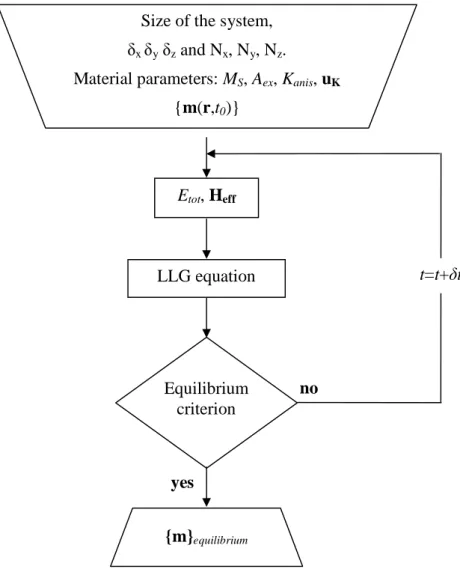
To synthesizethis paragraph, the flowchart of the GL_FFT software is presented in

Figure II.3. The first step is the initialization where the geometrical and the material parameters are given, together with the initial magnetization distribution. Then the energy terms and the surface and volume charges are calculated, and finally the effective field is obtained. This is then introduced in the LLG equation. After solving it, the criterion of

(m×Heff)/MS<10-6 rad is verified. If fulfilled, the equilibrium state is determined and the

(42)

Figure II.3: Flowchart of the GL_FFT software. Etot, Heff LLG equation Equilibrium criterion {m}equilibrium yes no t=t+δt Size of the system,

δx δy δz and Nx, Ny, Nz.

Material parameters: MS, Aex, Kanis, uK

New numerical approaches for micromagnetism and Current-induced domain wall motion

HAL Id: tel-00382710

https://tel.archives-ouvertes.fr/tel-00382710

Current-induced domain wall motion

Helga Szambolics

To cite this version:

Nouvelles formulations éléments finis pour le micromagnétisme

et

Déplacement de parois par courant polarisé en spin

Remerciements

Contents

Introduction

I.

Micromagnetic theory

( )

( )

I.1.

Energy functional

∑

(

)

( )

(

)

( )

∑

( )

(

)

(

( )

)

(

( )

)

∫

( )

(

)

∫

( )

( )

∫

(

)

(

)

(

)

( )

( )

( )

( )

( )

( )

( )

( )

( )

( )

( )

( )

( )

∫

∫

∫

∫

( )

(

) ( )

(

) ( )

[

]( ) [

]( )

∫

∫

( )

(

) ( )

(