Northern Hemisphere permafrost map based on TTOP modelling for
2000–2016 at 1 km
2
scale
Jaroslav Obu
a,⁎, Sebastian Westermann
a, Annett Bartsch
b, Nikolai Berdnikov
c,
Hanne H. Christiansen
d, Avirmed Dashtseren
e, Reynald Delaloye
f, Bo Elberling
g,
Bernd Etzelmüller
a, Alexander Kholodov
h, Artem Khomutov
c, Andreas Kääb
a,
Marina O. Leibman
c, Antoni G. Lewkowicz
i, Santosh K. Panda
h, Vladimir Romanovsky
h,j,
Robert G. Way
k,l, Andreas Westergaard-Nielsen
g, Tonghua Wu
m, Jambaljav Yamkhin
e, Defu Zou
m aDepartment of Geosciences, University of Oslo, Sem Sælands vei 1, 0371 Oslo, NorwaybZentralanstalt für Meteorologie und Geodynamik, Hohe Warte 38, 1190 Wien, Austria
cEarth Cryosphere Institute, Tyumen Scientific Center, Russian Academy of Sciences, Siberian Branch, Malygin street, 86, Tyumen 625000, Russia dArctic Geology Department, The University Centre in Svalbard, UNIS, P.O. Box 156, N-9171 Longyearbyen, Norway
eInstitute of Geography and Geoecology, Mongolian Academy of Sciences, P.O.B. 361, Ulaanbaatar 14192, Mongolia fGeography Unit, Department of Geosciences, University of Fribourg, Chemin du Musée 4, 1700 Fribourg, Switzerland
gCenter for Permafrost (CENPERM), Department of Geosciences and Natural Resource Management, University of Copenhagen, Øster Voldgade 10, 1350 Copenhagen, Denmark
hGeophysical Institute, University of Alaska Fairbanks, 2156 N Koyukuk Dr, Fairbanks, AK 99775, USA iDepartment of Geography, Environment and Geomatics, University of Ottawa, Ottawa, ON K1N 6N5, Canada jDepartment of Cryosophy, Tyumen State University, Tyumen, Russia
kDepartment of Geography and Planning, Queen's University, Kingston, ON K7L3N6, Canada
lLabrador Institute, Memorial University of Newfoundland, Happy Valley-Goose Bay, NL A0P1E0, Canada
mCryosphere Research Station on Qinghai–Xizang Plateau, State Key Laboratory of Cryospheric Science, Northwest Institute of Eco–Environment and Resources (NIEER), Chinese Academy of Sciences (CAS), 320 Donggang West Road, Lanzhou, Gansu, China
A R T I C L E I N F O Keywords: Permafrost map Ground temperatures Frozen ground Permafrost Remote sensing Cryosphere
Essential climate variable
A B S T R A C T
Permafrost is a key element of the cryosphere and an essential climate variable in the Global Climate Observing System. There is no remote-sensing method available to reliably monitor the permafrost thermal state. To es-timate permafrost distribution at a hemispheric scale, we employ an equilibrium state model for the temperature at the top of the permafrost (TTOP model) for the 2000–2016 period, driven by remotely-sensed land surface temperatures, down-scaled ERA-Interim climate reanalysis data, tundra wetness classes and landcover map from the ESA Landcover Climate Change Initiative (CCI) project. Subgrid variability of ground temperatures due to snow and landcover variability is represented in the model using subpixel statistics. The results are validated against borehole measurements and reviewed regionally. The accuracy of the modelled mean annual ground temperature (MAGT) at the top of the permafrost is ± 2 °C when compared to permafrost borehole data. The modelled permafrost area (MAGT < 0 °C) covers 13.9 × 10⁶km2(ca. 15% of the exposed land area), which is
within the range or slightly below the average of previous estimates. The sum of all pixels having isolated patches, sporadic, discontinuous or continuous permafrost (permafrost probability > 0) is around 21 × 106km2 (22% of exposed land area), which is approximately 2 × 10⁶km2less than estimated previously. Detailed
comparisons at a regional scale show that the model performs well in sparsely vegetated tundra regions and mountains, but is less accurate in densely vegetated boreal spruce and larch forests.
1. Introduction
Permafrost is a subsurface phenomenon that underlies a significant
part of the land and sea in the Northern Hemisphere (Brown et al., 1997;Rachold et al., 2007). Permafrost stores large amounts of organic carbon (Hugelius et al., 2014), affects the stability of bedrock and
⁎Corresponding author.
E-mail address:[email protected](J. Obu).
http://doc.rero.ch
Published in "Earth-Science Reviews 193(): 299–316, 2019"
which should be cited to refer to this work.
unconsolidated sediments, and impacts the costs and methods used for infrastructure development (Nelson et al., 2001;Gruber and Haeberli, 2009;Kääb, 2008;Hjort et al., 2018). Terrestrial permafrost monitoring is coordinated within the Global Terrestrial Network for Permafrost (GTN-P;Biskaborn et al., 2015), where ground temperatures are mea-sured in > 1000 boreholes, but only at discrete points. Extrapolating these observations to larger regions is hampered by the considerable spatial variability of the ground thermal regime and an uneven dis-tribution of sites that results in extensive unsampled areas (Biskaborn et al., 2015, 2019).
Despite its global significance, there is still no method to reliably detect the occurrence and extent of permafrost at medium to high spatial resolutions and at a global scale. While the occurrence of per-mafrost cannot be directly detected using remote sensing, satellite data can be used in characterizing permafrost extent and detecting changes indirectly using two different approaches (Westermann et al., 2015c): (1) remote identification and mapping of surface landforms that in-dicate the existence of permafrost, and (2) remote sensing of physical variables that relate to thermal subsurface conditions.
The first approach is usually restricted to local areas where per-mafrost landforms are evident so it cannot easily be applied globally. The second approach includes detection of the freeze-thaw state of the surface using passive microwave sensors (Kimball et al., 2001; Park et al., 2016;Kim et al., 2017;Xu et al., 2018;Kroisleitner et al., 2018) and modelling of permafrost using air or land surface temperatures (LST). Remotely sensed LSTs cannot be employed directly because of the insulating effect of the winter snow cover (e.g.Hachem et al., 2009) and the thermal offset between annual average LST and annual average ground temperatures caused by differing thermal conductivities of the active layer when frozen and thawed (Goodrich, 1978). However, permafrost models with varying complexity can be employed to relate LST to the ground thermal regime (Marchenko et al., 2009; Westermann et al., 2017).
The first comprehensive Northern Hemisphere permafrost extent map was compiled byBrown et al. (1997), based on national and re-gional maps and expert knowledge from different time periods and sources. This International Permafrost Association (IPA) map still re-presents the current state-of-the-art despite its inconsistencies for dif-ferent countries/regions and its limited spatial resolution. Several model approaches relating permafrost occurrence to surface meteor-ological parameters have been developed at regional scales (Boeckli et al., 2012;Jafarov et al., 2012; Nicolsky et al., 2017;Westermann et al., 2017). A first high-resolution (30 arc-second) estimate of the global permafrost zonation byGruber (2012)demonstrated the poten-tial for global permafrost mapping using simple semi-empirical schemes in combination with downscaled climate reanalysis data. Chadburn et al. (2017)extended this method and used climate model prediction outputs to estimate permafrost loss as a function of future atmospheric warming. Aalto et al. (2018) used statistical modelling to estimate current and future circum-Arctic ground temperatures at the depth of zero annual amplitude (ZAA) and active layer thicknesses.
High-resolution maps (up to 1 km2) have been successfully pro-duced using the TTOP (temperature at the top of permafrost) model for individual regions and countries. The model calculates mean annual ground temperature (MAGT) at the top of the permafrost based on mean annual air temperature (MAAT) and uses semi-empirical adjust-ment factors for the effects of snow cover and the thermal offset (Smith and Riseborough, 1996). The approach uses only a small number of input parameters and has been successfully employed at regional and continental scales for Canada (Smith and Riseborough, 2002;Way and Lewkowicz, 2016, 2018), Scandinavia (Gisnås et al., 2017) and China (Zou et al., 2017). These studies use regional datasets as input and parameter tuning to optimize model performance. For the North Atlantic region,Westermann et al. (2015a)employed globally available remotely-sensed satellite LST and reanalysis data as inputs to a TTOP model to estimate permafrost probability and ground temperatures at a
continental scale. To date, there has been no global modelling effort that is primarily based on observed LST and that can generate both permafrost temperature and permafrost zonation maps.
In this study, we extend and improve the remote sensing approach ofWestermann et al. (2015a)and apply a TTOP–based scheme to the entire Northern Hemisphere. Due to its simplicity and small number of required input parameters, the TTOP approach facilitates high-resolu-tion modelling, including a representahigh-resolu-tion of subpixel variability (Westermann et al., 2015a). We compile the first permafrost tempera-ture and zonation map at the circum-Arctic scale with a resolution of 1 km2that includes a statistical representation of subpixel variability of
permafrost temperatures based on snow and landcover heterogeneity. Outputs are validated against borehole temperature measurements and are compared to existing regional permafrost maps and other expert knowledge. The results complement existing permafrost zonation maps and observations of ground thermal state.
2. Methods
2.1. The Cryogrid 1 model
For calculation of mean annual ground temperature (MAGT), we use the CryoGrid 1 model (Gisnås et al., 2013), based on the TTOP equili-brium approach (Smith and Riseborough, 1996):
= + + + + >
(
)
MAGT n FDD r n TDD for n FDD r n TDD n FDD n TDD for n FDD r n TDD ( ) ( ) 0 ( ) 0 f k t f k t r f t f k t 1 1 1 k (1) Here, FDD and TDD represent freezing and thawing degree days, respectively, of the surface meteorological forcing accumulated over the model periodτ (in days). The influence of the seasonal snow cover, vegetation, and ground thermal properties are taken into account by the semi-empirical adjustment factors rk(ratio of thermal conductivity ofthe active layer in thawed and frozen state), nf(scaling factor between
winter air/surface and ground surface temperature) and nt (scaling
factor between summer air/surface and ground surface temperature). We use satellite-derived surface (skin) temperature to compute FDD and TDD (Fig. 1, and following section) instead of the air temperature in-itially used bySmith and Riseborough (1996, 2002)and hence set the thawing nt-factor to unity. Spatially distributed datasets based on
sa-tellite products and reanalysis are compiled (Fig. 1) for the other parameters and variables (TDD, FDD, nf, rk). The TTOP approach is
limited to near-surface permafrost and is unable to simulate relict or sub-sea permafrost.
2.2. TDD and FDD
We compile spatially distributed datasets of TDD and FDD from remotely sensed land surface temperature (LST) products. The Moderate Resolution Imaging Spectroradiometers (MODIS) on board the Terra and Aqua satellites have provided LST measurements at a spatial resolution of 1 km2since 2000 and 2002, respectively. The study period, therefore, starts in 2000 and extends to the end of 2016. We employ the MODIS MOD11A1 and MYD11A1 level 3 product in pro-cessing version 6, which contains up to two daytime and two night-time measurements per day (Wan et al., 2002;Wan, 2014).
Extended data gaps in the MODIS LST time series due to cloud cover can result in a systematic cold bias in seasonal averages (Westermann et al., 2012;Soliman et al., 2012;Østby et al., 2014). To prevent this, gaps are filled with near-surface air temperatures from the ERA-interim reanalysis which provides air temperature data throughout the study period at a spatial resolution of 0.75° × 0.75° (Dee et al., 2011). The validity of this gap-filling is supported by the similarity of air and
surface temperatures under cloudy skies (Gallo et al., 2010).
Downscaling of the ERA-interim reanalysis data to the 1 km2
re-solution of individual MODIS pixels is accomplished by computing at-mospheric lapse rates and the elevation difference between the ERA orography field and the elevation of a 1 km2pixel, similar to the
pro-cedure described inFiddes and Gruber (2014). The Global Multi-re-solution Terrain Elevation Data 2010 (GMTED2010) at 30 arcsec (ap-proximately 1 km2) resolution (Danielson and Gesch, 2011) is
employed for the elevation, while the ERA orography field is inter-polated to the centre of each MODIS pixel. Atmospheric lapse rates are computed from the near-surface air temperatures and the temperatures at 700 hPa pressure level, again interpolated to 1 km2pixels. For pixels where elevation exceeds the elevation of the 700 hPa pressure level, we successively employ the 500 hPa and 200 hPa pressure levels instead. The downscaled temperatures are then inserted into the gaps in the MODIS LST time series and the resulting time series is used to generate 8-day average temperatures from which FDD and TDD are finally ac-cumulated for the 2000–2016 study period.Westermann et al. (2017) showed that the cold bias of MODIS LST was significantly reduced after gap-filling, but a residual cold bias of approx. 1 K remained.
2.3. Snow water equivalent, snow depth and freezing nf-factors
To obtain a spatially distributed dataset of nf-factors, we first
gen-erate a 1 km2 dataset of mean annual snow depth (MASD) using a simple degree-day model forced by downscaled ERA-interim pre-cipitation and near-surface air temperature fields. Using the GMETD2010 DEM, precipitation is adjusted according to elevation differences between the ERA-Interim surface and the DEM elevation. Altitudinal precipitation gradients can vary considerably between dif-ferent regions (Körner, 2007), for instance with increases of 10% per 100 m (5% above 1000 m) in the seNorge snow model for Scandinavia (Mohr, 2008), whereasHevesi et al. (1992)suggests an increase only of 2% per 100 m in drier areas. We use a precipitation increase of 5% per 100 m elevation up to 1000 m above sea level (asl), and 2% per 100 m for elevations above 1000 m asl. Snowfall is defined as precipitation at air temperatures below 0 °C, based on the same downscaled ERA-In-terim air temperatures employed for gap filling of MODIS LST (see above), while snow melt is computed with a T-index model (Hock, 2003). To facilitate a global application, the range of degree day factors
reported in literature (2–12 mm d−1°C−1; Hock, 2003;Senese et al.,
2014) is scaled linearly according to a product of sun angle above horizon and day length. The sun angle above the horizon (θs, from
which also day length is obtained) is calculated as (Karttunen et al., 2016):
=90 + 23.45° ×sin 360 + 365 (284 DOY) s
(2) whereΦ denotes latitude and day of the year (DOY). Average snowfall and snowmelt are computed from downscaled ERA-Interim at 1 km2 spatial resolution for 12 h periods from which average yearly snow water equivalent (SWE) is accumulated for the study period. To convert SWE to snow depth, an empirical equation for average snow density based on field observations in the Northern Eurasia (Onuchin and Burenina, 1996) is employed.
= +
P 0323 0.00045HlnN 0.0447lnT (3)
Here, P denotes the snow density (g cm−3), N the snow cover period
in months, T the mean January temperature (°C) and H the average snow depth (cm), with H = SWE/P. The equation is rearranged to yield the average snow density P, so that the MASD can be calculated from SWE and the snow cover period obtained from the T-index model (see above). The mean January air temperature is approximated by the mean January surface temperature obtained from MODIS LST and ERA reanalysis (see above).
Freezing season nf-factors are calculated using the functional
re-lationships inSmith and Riseborough, 2002,Fig. 4) based on MASD and mean annual air temperature (MAAT). This nf-factor method was
shown to be less biased than using statistical approaches (Way and Lewkowicz, 2018). An ensemble of different values for MASD is con-sidered for each 1 km2grid cell (see “Subpixel Representation” below)
to account for subpixel spatial variability in snow depths (e.g.Gisnås et al., 2014). Mean annual surface temperatures from MODIS LST and ERA-Interim are employed as a proxy for MAAT.
2.4. rk-factors
The rk-factors greatly depend on water and organic contents (Smith
and Riseborough, 1996), providing physically-based constraints on their values (cf.Romanovsky and Osterkamp, 1995;Westermann et al.,
MODIS LST
temperaturesERA-InterimFDD and TDD
CCI Landcover
TTOP model
200 ensemble runs rk-factors
Mean MAGT Permafrost probability (fraction) Permafrost zones ERA-Interim temperatures Tundra wetness ERA-Interim precipitation nf-factors
Fig. 1. Flowchart of the employed methodology. The TTOP model was run 200 times with varying nf-factors and rk-factors according to subpixel statistics.
2015b). In this study, rk-values that are consistent with these
con-straints are assigned to landcover and soil moisture classes obtained from remote-sensing-derived gridded products.
For tundra regions, a dataset of site surface roughness which has been shown to be a suitable proxy for wetness (period 2002–2012; 500 m resolution, sensor ASAR GM;Widhalm et al., 2016) as well as soil organic carbon content (Bartsch et al., 2016) is used, defining rkvalues
for wet, medium wet and dry as 0.75, 0.85 and 0.95, respectively. Outside tundra regions, we use the ESA CCI Landcover product (period 2008–2012, version 1.6.1) with a horizontal resolution of approxi-mately 300 m and with rk-factors assigned to different landcover classes
(Table 1). These landcover groups are chosen based on classes em-ployed in previous regional TTOP analyses (Gisnås et al., 2017; Way and Lewkowicz, 2016).
The bare-ground landcover class rk-factor is set to 0.95 because it
often represents mountainous and soil-free locations with low moisture content, similar to a number of surficial deposits used byGisnås et al. (2017). The rk-factors are set to 0.95 and 0.9 for deciduous and
ever-green forest, which is similar toWay and Lewkowicz (2018)although lower rk-factors values can be found in forests with thick organic cover.
Rk-factor values around 0.5 have been reported in areas with thick
organic cover as in wetlands (Williams and Smith, 1989).
2.5. Ensemble-based modelling of subpixel heterogeneity
Permafrost extent and temperatures can vary considerably over short distances due to heterogeneous snow cover, vegetation, terrain and soil properties (Beer, 2016;Cable et al., 2016;Gisnås et al., 2014, 2016;Zhang et al., 2014). To simulate this variability, we run an en-semble of 200 model realizations with different combinations of nfand
rk-factors that are selected according to subpixel statistics for the
landcover classes and a typical distribution of snow depths within the 1 km2 pixel. A log-normal distribution function is used to obtain an
ensemble of snow depths (Pomeroy et al., 1998;Faria et al., 2000), with MASD determining the average of the distribution. The coefficients of variation of the distribution are assigned according toListon (2004), using groups of landcover classes (Table 2).
Subpixel landcover statistics that provide an ensemble of rk-values
are deterministically calculated from 300 m2CCI Landcover pixels (see
above), adding a variation of ± 0.05 to the rk-factors in each class. If at
least 90% of a pixel is classified as water body or permanent snow and ice, it is masked out. Unique values of nfand rkare stochastically drawn
for 200 ensemble members inside each 1 km2pixel. The resulting
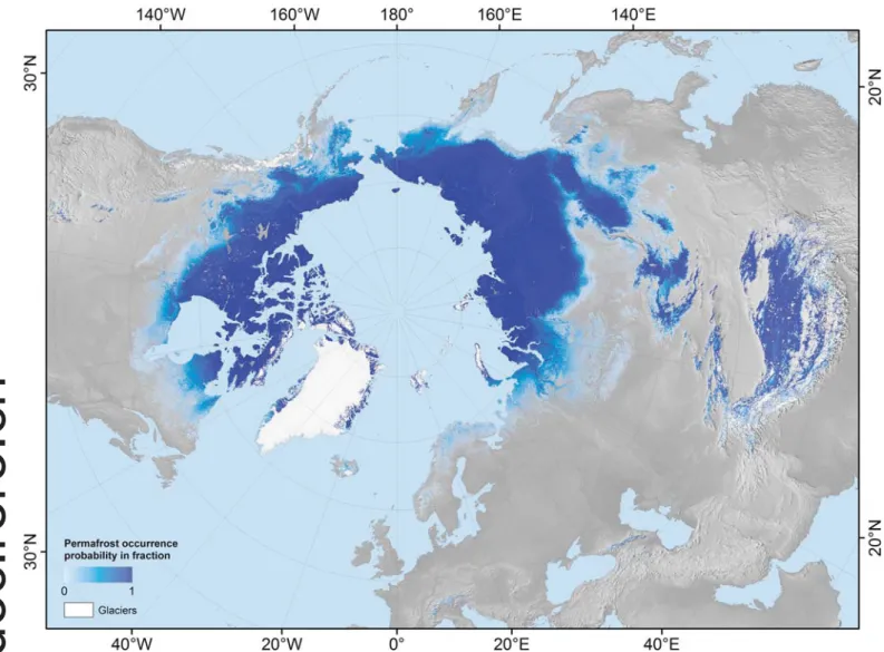
en-semble of MAGT is obtained through Eq. (1), allowing permafrost probability (1 corresponding to 100%) to be calculated as the fraction of ensemble members with MAGT of 0 °C or lower. This fraction also corresponds to the modelled percentage of the 1 km2 pixel area
un-derlain by permafrost, so that it can be directly compared to permafrost zones of the IPA map (Brown et al., 1997). The permafrost probability is subsequently classified into: continuous permafrost (> 0.9), dis-continuous permafrost (0.5–0.9), sporadic permafrost (0.1–0.5) and isolated patches (0.005–0.1). The zonal classification is generalised using an ArcGIS focal statistics rectangular 5 × 5 filter and boundary clean tools before being vectorised.
The GlobPermafrost map is used below as a term to encompass all of the model outputs (named after European Space Agency project). Permafrost area is defined as the area of MAGT below 0 °C while per-mafrost region refers to areas where the perper-mafrost probability is > 0, which includes the area of all permafrost zones (Zhang et al., 2000). The term permafrost extent is used in relation to both permafrost area and permafrost region. The extent of the permafrost region is larger than that of the permafrost area because a pixel with an ensemble average MAGT > 0 °C can still have permafrost probability > 0 due to subpixel variability, so that pixel is within the permafrost region but is not part of the permafrost area.
2.6. Model validation
We compare our ensemble MAGT mean to in-situ point measure-ments in 359 boreholes in the GTN-P (Global Terrestrial Network for Permafrost, Biskaborn et al., 2015) and 392 boreholes in the TSP (Thermal State of Permafrost) project network (Romanovsky et al., 2010). In addition, we use a collection of 169 MAGT measurements from China (Jin et al., 2007;Wu et al., 2007a;Wu et al., 2007b;Wu and Zhang, 2008;Wu et al., 2010;Wu et al., 2012;Luo et al., 2012;Chang et al., 2013;Wu et al., 2015;Wang et al., 2017;Qin et al., 2017;Luo et al., 2018;Liu et al., 2017) and from Scandinavia and Iceland (Farbrot et al., 2007, 2013). The GTN-P database contains more recent borehole data compared to the TSP (measured during the International Polar Year from 2007 to 2009). Therefore, TSP boreholes within a 500 m radius of GTN-P boreholes are not used. In the same manner, GTN-P and TSP boreholes are excluded from the comparison when they are ad-jacent to boreholes in the Chinese dataset. Root mean square errors (RMSE) and mean differences are calculated for all borehole sites within natural geographical regions. The GlobPermafrost map is also put into the context of regional permafrost maps, which are compiled during various time periods and different production approaches.
3. Model results and their regional reviews
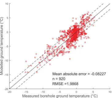
3.1. Comparison to global borehole networks and permafrost maps The comparison to borehole measurements shows a mean absolute error of −0.08 °C, which is partly due to a fine-tuning of rk-factors,
while a RMSE of 1.99 °C is evidence of the differences between model and measurements (Fig. 2). For 35% of the boreholes, the agreement between borehole temperatures and modelled MAGT is better than 1 °C,
Table 1
List of rk-factors assigned to landcover class groups and CCI landcover class
used to create landcover class groups.
Landcover class group rk-factor CCI Landcover classes
Bare areas 0.95 140, 150, 152, 153, 200, 201, 202 Grasslands and croplands 0.75 10, 11, 12, 20, 130
Shrubs 0.8 30, 40, 100, 110, 120, 121, 122 Deciduous forest 0.95 50, 60, 61, 62, 80, 81, 82, 90 Evergreen forest 0.9 70, 71, 72 Wetlands 0.55 160, 170, 180 Urban 0.7 190 Table 2
Coefficients of variation for snow distribution (Liston, 2004) assigned to landcover class groups and CCI landcover classes used to create landcover class groups.
Landcover class group Coefficient of variation CCI Landcover classes
Open 0.9 10, 11, 12, 20, 130, 140, 150, 152, 153, 190, 200, 201, 202, 220 Shrub 0.4 30, 40, 100, 110, 120, 121, 122 Forest 0.2 50, 60, 61, 62, 70, 71, 72, 80, 81, 82, 90 Wetland 0.4 160, 170, 180 Water 0.4 210
http://doc.rero.ch
while it is better than 2 °C for 69%, and better than 3 °C for 87% of the boreholes. Most RMSE values for regional subdomains are < 2.0 °C, except for Canada, Alaska, and the Asian part of Russia, where they are still < 2.5 °C. For Canada and China, the average MAGT is under-estimated by around 1 °C, while it is overunder-estimated between 1 and 1.5 °C for Svalbard, Scandinavia and Greenland.
Assuming a Gaussian distribution of MAGT standard deviation (SD), 68% of borehole comparisons should fall within one SD, while 95 and 99% should be within two and three SDs, respectively. Our comparison shows 375 (41%) boreholes are contained within one, 622 (68%) within two and 752 (82%) within three SDs from the mean, which is similar to the numbers thatWestermann et al. (2015a)obtained for a much smaller domain (47%, 75%, 90%).
3.2. Permafrost extent and MAGT
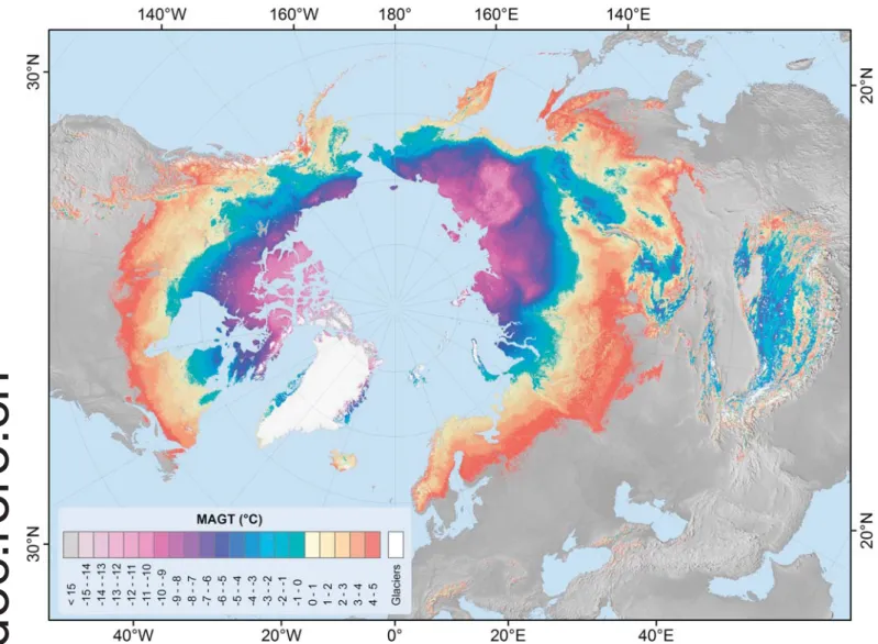
The best estimate of the permafrost area in the Northern Hemisphere is 13.9 × 10⁶km2(14.6% of the exposed land area),
re-presenting the total area with where MAGT < 0 °C (Fig. 3). The bore-hole temperature comparison can be used to incorporate uncertainty into this estimate, giving a minimum permafrost extent of 10.1 × 10⁶km2 (10.5% of exposed land area; the area within MAGT < −2 °C) and a maximum extent of 19.6 × 10⁶km2(20.6% of exposed land area; the area within MAGT < +2 °C). The extent of the permafrost region (i.e. all permafrost zones) inferred from permafrost occurrence probabilities is 20.8 × 10⁶km2 (21.8% of exposed land area). The continuous permafrost zone occupies about half of this area, underlying 10.7 × 10⁶km2 (11.2% of exposed land area), while the
discontinuous (3.1 × 10⁶km2; 3.3% of exposed land area), sporadic (3.5 × 10⁶km2; 3.6% of exposed land area), and isolated patches zones
(3.5 × 10⁶km2; 3.6% of exposed land area) almost equally divide the
remainder.
The permafrost zonation boundaries, which in this study correspond to permafrost probability values (Figs. 4 and 5), are associated with particular MAGT values. The average modelled MAGT at the boundary between continuous and discontinuous permafrost is −1.71 ± 0.48 °C, at the discontinuous/sporadic boundary it is −0.01 ± 0.37 °C, and at the sporadic/isolated-patches boundary it is 1.46 ± 0.44 °C. The last isolated patches of permafrost occur at average modelled MAGT of 2.62 ± 0.53 °C.
3.3. Standard deviation
The MAGT SD (corresponding to the spread of the model ensemble) is highest in the open and wetlands landcover groups with an average SD of 1 °C, and lowest in the forest and shrub landcover groups to the south with SD of 0.5 and 0.4 °C, respectively. The low SDs south of tundra regions represent forest and shrub landcover groups. The SD in the open landcover group varies greatly between arctic tundra regions (SD be-tween 2.0 and 2.5 °C) and mountainous regions such as the European Alps, Scandinavian Mountains, the Caucasus, the Rocky Mountains, the Himalaya and the Tian Shan (SD usually below 1 °C,Fig. 6).
Because the FDDs and TDDs are constant in all model runs, the MAGT variation is due to different nf- and rk-factors. The differences in
SD between the forest and open landcover groups are due to a low coefficient of variation set for the snow distribution. The differences within the open landcover group mainly relate to differences in snow cover. The nf-factors are most variable at low snow depths while they
change little once the snow cover is thick. The SDs reach 3.5 °C on Ellesmere Island and in northern Greenland where the input snow cover is very thin. Few studies have evaluated the real spatial variability within the area of a modelled pixel, butGisnås et al. (2014) showed MAGST differences up to 6 °C due to difference in snow cover within 1 km2andGruber et al. (2017)measured MAGT differences up to 2.5 °C
within 15 × 15 m plots due to differences in surficial geology, vegeta-tion, drainage conditions, and snow accumulation.
3.4. Regional results and review of permafrost extent and MAGTs The modelled results are compared to borehole measurements and existing regional permafrost maps, which were produced at different time and spatial scales and are based on various mapping techniques. For this reason, only the comparisons with borehole data can be treated as a validation while comparisons to other maps show only relative differences among them.
3.4.1. Russia
Our results for Russia show a temperature bias of 0.2 °C when compared to borehole temperatures. However, a RMSE of 2.1 °C (n = 287) indicates significant regional differences. The model perfor-mance is better for the European part of Russia (RMSE 1.4 °C; n = 82) than for the Asian part (RMSE 2.4 °C; n = 205). Comparison in the area east of Ural Mountains reveals that modelled MAGT is overestimated with an average warm bias of 0.4 °C and SD of 1.2 °C, but is under-estimated by approximately 1 °C on Pay-Khoy ridge and the coastal plain northwest of the Polar Urals. The modelled MAGT is over-estimated by 1–3 °C on Yamal, Tazovsky and Gydan Peninsulas but sites show both positive and negative MAGT differences close to the southern limits of permafrost. The MAGT is considerably under-estimated in the continental part of Siberia with differences ranging between 1 and 6 °C. The boreholes in the vicinity of Yakutsk show MAGT underestimation by an average of 4 °C. However, slight MAGT overestimation is observed at the Siberian sites by the Arctic Ocean. The modelled MAGT is also warmer in the southern part of Far East Russia (by 2–4 °C), the Amur region (1 °C on average) and Kamchatka (up to 3 °C).
The results (Fig. 7) can also be compared to the MAGT at the ZAA on the Geocryological map of the USSR (scale 1:2,500,000, digitised to 100 m2pixels) compiled in 1991 (Kondratieva et al., 1996), and re-presenting several decades before the 2000–2016 period (Supplemen-tary Fig. S1). The permafrost extent appears to be overestimated in the Ob River floodplain, which is classified as wetland in the CCI landcover. The southern limits of permafrost are modelled north by 30–40 km at the Pechora River and 80 km in the area close to the Ural Mountains. As a result of mean MAGT overestimation in West-Siberian regions, the southern limit of permafrost is modelled about 100 km farther north compared to the Geocryological map. The areas at the southern
-20 -15 -10 -5 0 5 10
Measured borehole ground temperature (°C)
-20 -15 -10 -5 0 5 10
Modelled ground temperature (°C) Mean absolute error = -0.08227
n = 920 RMSE =1.9868
Fig. 2. Measured vs. modelled TTOP ground temperatures for all boreholes.
The dashed lines represent ± 2 °C intervals around the 1:1 solid line.
permafrost limit (south of Taimyr) show mostly MAGT overestimation, so that the resulting permafrost limit is shifted about 500 km to the north-east. The southern limit of permafrost is for the same reason shifted towards the north of Okhotsk Sea by 150 km compared to the Geocryological map. The extent of continuous permafrost in Eastern Siberia and Russian Far East is similar in both maps, except for the Chukotka and Magadan regions (North-East Russia), where extent is smaller in the GlobPermafrost map.
3.4.2. Canada
The average difference between borehole temperatures in Canada and predictions is −1.1 °C with an RMSE of 2.2 °C (n = 130). The re-sults are highly correlated for the entire set of Canadian boreholes (r2= 0.75; n = 130), but the correlation is significantly lower (r2= 0.27; n = 108) for MAGTs above −5 °C (Supplementary Fig. S4).
For borehole temperatures just below 0 °C, modelled temperatures vary from −5 to +3 °C, while the largest systematic differences between modelled and borehole MAGTs occur above 0 °C. Borehole temperature clustering is apparent in western Canada with modelled MAGTs almost all warm-biased (up to 1.7 °C) in the southern Yukon and almost all cold-biased (up to 5 °C, 2 °C on average) within the Mackenzie Valley (Northwest Territories), resulting in corresponding under- and over-prediction of permafrost probabilities, respectively. Overall, the accu-racy of permafrost presence in our model is lower in the sporadic permafrost zone of subarctic Canada and higher in Arctic Canada where
permafrost is continuous.
Our modelling predicts that 34–46% of the land area of Canada (3.0 × 10⁶km2to 4.0 × 10⁶km2) is underlain by permafrost (Fig. 8), similar to the estimate of 33–47% byBrown et al. (1997). The spatial pattern of permafrost zonation across Canada in this study, such as the substantial shift of permafrost zones northward on the eastern side of Hudson Bay, is similar to the Permafrost Map of Canada (Heginbottom et al., 1995), representing the 50-year period prior to our study period. The boundary of the continuous permafrost zone, however, is displaced southwards across much of the Northwest Territories and northern Manitoba compared to Heginbottom et al. (1995), more closely re-sembling the southern boundary of the discontinuous permafrost zone (Supplementary Fig. S3). In contrast, continuous permafrost on the shore of Hudson Bay in northern Ontario appears under-represented while the continuous permafrost in northern Manitoba and sporadic permafrost in parts of northern Ontario modelled byZhang et al. (2012) andOu et al. (2016)is generally reproduced. Discontinuous permafrost across much of the boreal forest zone is less widespread compared to Heginbottom et al. (1995), particularly in the southern Yukon and northern Ontario. In the high mountain areas in southern Alberta, the GlobPermafrost map shows significantly more detail in the permafrost distribution due to the better spatial resolution. For comparisons to regional permafrost maps see supplemental material.
Fig. 3. Average MAGT at TTOP of all model realizations for the Northern Hemisphere. Glacier/ice-sheet areas are extracted from the ESA CCI Landcover product.
Background topography is from the GMTED2010 elevation model.
3.4.3. Alaska
Our MAGT is modelled as 0.4 °C too warm relative to the borehole data with a relatively high RMSE of 2.08 °C (n = 174). The increase of permafrost temperature along a North-South transect is not very clearly captured by our modelled MAGT. The modelled mean MAGT is close to −6.0 °C near the coast (mean MAGT: Barrow: −6.2 °C; West Dock: −6.6 °C) and colder mean MAGT values were modelled further inland (Franklin Bluff: −7.2 °C; Galbraith Lake: −7.2 °C), which however re-mains inside the RMSE band. Overall, mean MAGT values for most of Alaska (i.e. south of the North Slope) appear warm biased.
In comparison to the “Permafrost Characteristics of Alaska” map (Jorgenson et al., 2008; based on surficial geology and the PRISM cli-mate map), the permafrost extent matches well in northern Alaska (i.e. North Slope of Alaska) and southwestern Alaska (Fig. 8). However, the boundary between continuous and discontinuous permafrost is shifted northwards in our product. Permafrost is continuous in the northern part of the Seward Peninsula and discontinuous in the southern part in Jorgenson et al. (2008), while it is modelled as discontinuous in the northern part and as sporadic in the southern part in our product. In contrast, the extent of the isolated patches zone in central Alaska ap-pears to be overestimated by our model. Permafrost is absent south of Katmai National Park and in Kodiak Island, but patches of dis-continuous or isolated permafrost south of Katmai National Park are modelled. Overall, the GlobPermafrost map shows a smaller permafrost extent in Alaska than the Permafrost Characteristics of Alaska map.
3.4.4. China
In comparison to borehole measurements, our modelled MAGT is underestimated on average by −0.94 °C (n = 188) with an RMSE of 1.76 °C. The MAGT is mainly overestimated (up to 3 °C) in northeastern China although under- and overestimations in the Daxinganling Mountains are relatively small. The majority of the Chinese boreholes (n = 151) are located in the eastern part of the Tibetan Plateau, where MAGT is moderately, but consistently underestimated (1.5 °C on average), which significantly influences the Chinese average. The MAGT was mainly overestimated in the western part of Tibetan Plateau. In comparison to permafrost maps in northeastern China (Guo et al., 1981;Zhou and Guo, 1982;Zhou et al., 1996;Wei et al., 2011,Luo et al., 2014a, 2014b), the GlobPermafrost map (Fig. 9) reproduces the continuous and discontinuous permafrost in the Daxinganling Moun-tains, sporadic permafrost in Xiaoxinganling Mountains and southern permafrost limit in both. Comparison to Tibetan Plateau permafrost map (period 2003–2012, TTOP model based on regional datasets) (Zou et al., 2017) shows a substantial agreement between both datasets (Supplementary Table S1) with differences occurring mainly at the margins of the continuous permafrost zone (Supplementary Fig. S6). The permafrost distribution also matches well with the “Map of Snow, Ice and Frozen Ground in China” (Shi and Mi, 1988) in both the Altai Mountains and the Tien Shan, except for the Youledusi Basin in the central Tien Shan, where discontinuous and sporadic permafrost is modelled, while the Chinese map does not indicate the existence of permafrost (Supplementary Fig. S7).
Fig. 4. Permafrost probability calculated as the fraction of model runs with MAGT below 0 °C.
3.4.5. Mongolia
The comparison to 36 boreholes shows a negative temperature bias of −0.31 °C and RMSE of 1.36 °C. The MAGT is slightly overestimated according to 11 borehole sites in Khentii Mountain (0.6 °C on average) and moderately underestimated in the area between Khangai Mountains and Shishged River (1.0 °C on average, n = 22). Three borehole temperatures in the northern part of Altai Mountains show average MAGT overestimation of 1.8 °C. Permafrost presence is cor-rectly modelled at 82% of 109 local observation sites, but some of these are located in small permafrost patches that are not captured by the model resolution.
Permafrost extent in the high altitude regions in Altai Mountains is similar to that in the permafrost map of Mongolia (Jambaljav et al., 2017; Supplementary Fig. S8) which is based on TTOP modelling using MODIS LST and local datasets. Our results indicate sporadic and dis-continuous permafrost in the Uvs Lake depression but both field studies and the Mongolian map do not show permafrost there. Permafrost presence is modelled in the mountain regions of Dariganga Plateau and Gurvan Saikhan, where the Mongolian permafrost map again does not show permafrost. However,Gravis et al. (1971)reported permafrost presence in both regions, although this was not confirmed by recent observations. The modelled permafrost extent is underestimated in Shishged River Valley and the northwest side of Khentii Mountain, which are covered by forest and moist organic soil layers that favour permafrost existence (Etzelmüller et al., 2006;Dashtseren et al., 2014)
and are likely not captured by the TTOP approach. 3.4.6. Scandinavia
On average, the modelled MAGT is overestimated by 1.3 °C (RMSE = 1.73) in comparison to 35 boreholes. The model results are generally too warm in mountain areas with thin snow cover, whereas some fit well and a few are modelled as too cold (Tron, Tarfala, Lavkavagge 2, Guloas 2, 3, Kistefjellet). The latter are in the areas of thick snow cover and where winter temperature inversions occur (Farbrot et al., 2013;Westermann et al., 2013)
The general permafrost distribution patterns in Scandinavia accord well in the GlobPermafrost map (Supplementary Fig. S9) and the Nordic permafrost map (Gisnås et al., 2017). However, the GlobPermafrost map shows less continuous and discontinuous permafrost in mountai-nous regions of southern Norway, northern Sweden, inner Troms and the Gaissane Mountains in Finnmark. On the other hand, the extent of sporadic permafrost appears greater in the areas southeast of Rondane and Valdresflya, and lowland areas of northern Norway, Sweden and Finland, where permafrost is mainly present in palsa mires. The greater extent of sporadic permafrost might be due to the overrepresentation of wetlands in the CCI landcover or due to strong temperature inversions that previous modelling approaches did not take into account. 3.4.7. Svalbard
The modelled MAGTs are in Svalbard higher than measured
Fig. 5. Permafrost zonation based on classified modelled permafrost probabilities (Fig. 4) which correspond with the fraction of each 1 km2pixel underlain by
permafrost.
borehole temperatures (mean difference of 1.48 °C, n = 19, RMSE = 1.93). The MAGT overestimation varies greatly among land-forms, as these have highly variable snow depths and ground ice con-tents (Christiansen et al., 2010). This variability is captured in the en-semble spread but not in the mean MAGT.
Permafrost is traditionally classified as continuous throughout the archipelago (Brown et al., 1997), but the modelled results indicate presence of discontinuous permafrost in the coastal areas of western Spitsbergen and some larger lowland valley areas. This is in accordance with previous modelling studies that indicated the potential formation of taliks in the lowlands (Etzelmüller et al., 2011), and recent warming trends observed in lowland coastal areas in western Svalbard, partly due to reduced sea ice cover (Isaksen et al., 2016;Christiansen et al., 2019). This partly accords with the increasing permafrost borehole temperatures at the west coast of Svalbard, to date reaching close to −3 °C at around 10 m depth (Christiansen et al., 2019).
3.4.8. Iceland
The agreement between the modelled and measured MAGT in four boreholes is good (mean difference = 0.53 °C, RMSE = 0.90). The modelled MAGT is underestimated by 0.6 °C in the mountains close to Vopnafjörður, where the borehole is situated in a snow drift and overestimated in the Egilsstaðir by 1.3 °C. The modelled MAGT accords well with the measured MAGT in the other two boreholes.
The spatial distribution of the permafrost zonation in Iceland (Supplementary Fig. S9) is similar to previous studies (Etzelmüller
et al., 2007;Farbrot et al., 2007) in the northern part around Tröllas-kági and southwards towards Hágöngur, while permafrost abundance appears to be slightly exaggerated in the southern and south-eastern part of Iceland. The area where palsas occur (as described inArnalds, 2008) is identified, but the modelled extent of isolated patches is greater. Permafrost in the southeast (Egilsstaðir) appears better re-presented by the GlobPermafrost map than by previous attempts (e.g. Farbrot et al., 2007), based on field measurements in the area. The GlobPermafrost map indicates discontinuous permafrost at higher ele-vations on the Vestfjord Peninsula where permafrost presence is con-firmed by landslides originating in a frozen debris cover (Sæmundsson et al., 2018).
3.4.9. Greenland
The distribution of permafrost in the Greenland is controlled by the overall climatic zonation from north to south and regional climatic gradients from the coast to the Greenland Ice Sheet. The comparison of our MAGT values to seven boreholes, which are distributed across all climate zones in Greenland, yields satisfactory results with average temperature overestimation of < 1.0 °C and an RMSE of 1.6 °C. Modelled MAGT is too high except for the inland site of Kangerlussuaq close to the Greenland Ice Sheet. Further validation with additional six independent sites confirms good model performance and robustness in Greenland (Supplementary Fig. S10).
Although the permafrost zonations from GlobPermafrost and Westergaard-Nielsen et al. (2018) were derived differently (see
Fig. 6. Standard deviation of MAGT at TTOP derived from 200 ensemble runs.
supplement), there is a considerable agreement between them (Sup-plementary Figs. S11 and S12). Differences in the distribution of per-mafrost types between these two maps (Supplementary Fig. S13) are mainly in South Greenland between 59 and 65°N where continuous permafrost is modelled in our study, whereas theWestergaard-Nielsen et al. (2018)map shows only 15% of the area as continuous permafrost. An earlier map (Christiansen and Humlum, 2000) does not show per-mafrost in southern Greenland, while the GlobPerper-mafrost map indicates sporadic permafrost. On the other hand, the GlobPermafrost map shows isolated patches in coastal areas up to 70°N on the east coast of Greenland, where both of the previous maps indicate predominantly discontinuous permafrost. On the west coast, GlobPermafrost map shows more extensive continuous permafrost in the central part (67°–68°N) compared to the two earlier maps, which mainly have dis-continuous permafrost in this area. These variations can be explained by the definition of permafrost zones in earlier maps, which are often set to indicate continuous permafrost in areas with MAAT below −5 °C and discontinuous permafrost in areas with MAAT between −5 and − 2 °C.
3.4.10. European Alps
The MAGT in the Alps is overestimated by 0.9 °C (n = 35, RMSE = 1.48 °C) when compared to borehole measurements. The crepancy is small especially when considering a strong thermal dis-equilibrium caused by air temperature warming over the last 25–30 years. The MAGT difference is smaller than 1 °C at 18 sites and it
is slightly > 2 °C only at 6 sites. The site in Swiss Alps, where MAGT is overestimated by 4 °C, is located in an extra-zonal permafrost.
The GlobPermafrost map (Supplementary Fig. S14) mimics the pattern of permafrost distribution shown in the high resolution Alpine Permafrost Index Map (Boeckli et al., 2012). Only isolated areas in the class “Permafrost only in very favourable categories”, which commonly represent steep rock walls and extra-zonal permafrost sites, are absent from the GlobPermafrost map.
3.4.11. Other mountain areas
Permafrost distribution is modelled for several mountainous areas outside the regions described above. All permafrost zones occur in the Rocky Mountains of the USA with sporadic permafrost in Colorado at elevations above 3200 m asl and discontinuous permafrost above 3500 m asl, results which agree with observations byIves and Fahey (1971). Isolated permafrost patches are modelled in the highest peaks of the Sierra Nevada in the southwestern USA, which corresponds well with the presence of active rock glaciers in the area (Liu et al., 2013). The model predicts sporadic permafrost for the highest parts of the Pyrenees Mountains, above 2500 m asl.Serrano et al. (2001)showed permafrost presence there above 2700 m asl. No permafrost is modelled in the Sierra Nevada, Spain, whereGómez et al. (2001)located per-mafrost remnants, but the lowest MAGTs from the ensemble spread are close to 0 °C.
Permafrost extent is successfully modelled for eastern and south eastern Europe. Small areas are correctly modelled for the Southern
Fig. 7. GlobPermafrost zonation, permafrost extent afterBrown et al. (1997)and difference between borehole and modelled MAGT for Russia. Negative values indicate model MAGT underestimation and positive values indicate overestimation. (For interpretation of the references to colour in this figure legend, the reader is referred to the web version of this article.)
Carpathians, where permafrost is present above 2000–2100 m asl (Urdea, 1998) and for the Tatra Mountains where isolated permafrost patches start to occur above 1900 m asl (Moscicki and Keîdzia, 2001). The model correctly reproduces permafrost presence in the Balkan Mountains above 2300 m asl (Dobiński, 2005).
Permafrost is modelled in several mountainous areas in Turkey: above 3100 m asl in the Taurus Mountains and above 2600 m asl in the Pontus Mountains. The existence of permafrost in these two regions is indicated by active rock glaciers (Kargel et al., 2014). According to our results, permafrost starts at between 2600 and 2800 m asl in the casus Mountains and between 2700 and 3000 m asl in the South Cau-casus Mountains. These elevations are lower than the limits estimated byGorbunov (1978). Permafrost is inferred to begin at 3400 m asl on Sabalan Mountain and at around 3600 m asl in the Elburz Mountain Range in Iran, which is again lower than estimated by Gorbunov (1978).
Isolated patches of permafrost are modelled for the Daisetsu Mountains, Hokkaido, Japan, above 1800 m asl.where Ishikawa and Hirakawa (2000) reported permafrost presence above 1750 m asl. Continuous permafrost is modelled for the peak of Mt. Fuji, where permafrost has been confirmed byHiguchi and Fujii (1971). Isolated patches of permafrost are also modelled for the Japanese Alps above 2500 m asl.
Isolated patches of permafrost are modelled for the Daisetsu
Mountains, Hokkaido, Japan, above 1800 m a.s.l. whereIshikawa and Hirakawa (2000) reported permafrost presence above 1750 m a.s.l. Continuous permafrost is modelled for the peak of Mt. Fuji, where permafrost has been confirmed byHiguchi and Fujii (1971). Isolated patches of permafrost are also modelled for the Japanese Alps above 2500 m a.s.l.
4. Discussion
The GlobPermafrost map is the first to portray both ground tem-perature and permafrost zones at circum-Arctic scale using a TTOP model based primarily on remote sensing dataset with a spatial re-solution of 1 km. Here we discuss the model limitations, outputs and influence of input data on results.
4.1. Model performance and limitations
The TTOP framework is an equilibrium model that does not take into account the history of ground thermal conditions before the study period, nor changes of ground temperature under a warming climate. This can affect its accuracy where permafrost is rapidly warming or cooling, especially where ground temperatures approach 0 °C and the soil moisture content is high. In such cases, the disequilibrium between atmospheric and ground temperatures increases because latent heat
Fig. 8. GlobPermafrost zonation, permafrost extent afterBrown et al. (1997)and difference between borehole and modelled MAGT for Canada and Alaska. 1: Katmai National Park; 2: Barrow; 3: West Dock and Deadhorse; 4: Franklin Bluff; 5: Galbraith Lake. (For interpretation of the references to colour in this figure legend, the reader is referred to the web version of this article.)
effects slow down potential thaw (Smith et al., 2005, 2010). Numerous measured borehole temperatures are close to 0 °C (Fig. 2) which makes disequilibrium with surface climate possible at these sites. The magni-tude of the disequilibrium is associated with the persistence of relict permafrost rather than the ratio of frozen to thawed thermal con-ductivities (James et al., 2013;Throop et al., 2012). The occurrence of relict permafrost cannot be simulated for this reason and permafrost extent may be underestimated in areas where it persists deeper in the ground beneath a talik. Such transient conditions may persist for dec-ades until TTOP values eventually exceed 0 °C or for centuries if the relict permafrost layer is thick. In the interim, the measured borehole MAGT would be colder than modelled MAGT, as could be the case for example, in much of the southern Yukon (Fig. 8).
Exclusion of nt-factors from the model enabled us to use
high-re-solution MODIS LST data, but may have reduced the model perfor-mance in forested regions where the inputs represent the temperature of the tree canopy rather than ground surface. The percentage of MODIS LST measurements included in FDD and TDD calculation also depends on the cloudiness of the area. The fused MODIS LST and ERA-Interim time series likely don't represent the microclimates of dense forests well and these also vary among different forests types (Vanwalleghem and Meentemeyer, 2009).
The model does not account for permafrost variability in steep mountains due to aspect and topography. Elevation and aspect sub-grid variability are especially important for permafrost distribution in mountainous areas (Gruber and Haeberli, 2009), but the MODIS LST is
measured from space and contains little signal from steep slopes and no signal from vertical walls. The model is also not able to simulate the absence of snow on steep mountain slopes. There are no studies that describe relationships between elevation, aspect and MAGT at scales relevant for our work, precluding their representation as terrain sub-pixel variability within the TTOP model. This could be a reason for the MAGT mismatch in the mountains of Eastern Siberia, but on the other hand, the model performed well for the European Alps and other mountainous regions outside the Arctic. We therefore assume that the modelling results are satisfactory in most mountainous regions, al-though validation is lacking where few permafrost studies have been conducted (e.g. the Caucasus, Turkey and Middle Asia).
Permafrost properties are known to vary considerably within 1 km2 grid cells (Schmid et al., 2012; Gisnås et al., 2014). The ability to partially represent this variability at a spatial resolution of 1 km2using
subpixel landcover information is crucial for model accuracy and in particular for comparison to borehole data. A previous TTOP statistical modelling approach byWestermann et al. (2015a)used a single land-cover value and snow thickness values to define possible ranges of nf
and rk-factors for a pixel. The GlobPermafrost approach takes into
ac-count all landcover classes present within a 1 km2 MODIS pixel for
defining nfand rkvalues. We note that extra-zonal permafrost
occur-rence in talus slopes or ice caves is not represented by the GlobPer-mafrost map as their special site conditions and processes are typically not represented in the input data and the TTOP model, respectively.
Fig. 9. GlobPermafrost zonation, permafrost extent afterBrown et al. (1997)and difference between borehole and modelled MAGT for China and Mongolia. Note: permafrost extent afterBrown et al. (1997)is misplaced in some areas 1: Youledusi Basin; 2: Uvs Lake; 3: Shishged River; 4: Dariganga Plateau; 5: Gurvan saikhan. (For interpretation of the references to colour in this figure legend, the reader is referred to the web version of this article.)
4.2. Permafrost extent and MAGT
Our estimate of 13.9 × 10⁶km2for permafrost area (MAGT < 0 °C) in the Northern hemisphere is within the range of or lower than the middle values reported in previous studies.Zhang et al. (2000) esti-mated the Northern Hemispheric permafrost area to between 12.2 and 17.0 × 10⁶km2based on the IPA map zone fractions.Gruber (2012)
estimated the permafrost area to range between 12.9 and 17.7 × 10⁶km2 using a semi-empirical modelling scheme based on downscaled climate reanalysis data. Our permafrost area range calcu-lated based on a MAGT RMSE of ± 2 °C is larger than the latter.Aalto et al. (2018)produced circum-Arctic MAGT at ZAA and active layer thickness, and estimated the permafrost extent to be around 15.1 ± 2.8 × 10⁶km2, a value which is close to our estimate. They
reported an RMSE of 1.6 °C, which is lower than our estimate but the models differ significantly since the results are fitted to validation data using statistical forecasting.
The extents of the permafrost region (area of all permafrost zones) estimated by Zhang et al. (2000) and Gruber (2012) are 22.8 and 21.7 × 10⁶km2, respectively, while our estimate of 20.8 × 10⁶km2is
about 2 × 10⁶km2(2% of exposed land area) lower than these two.
Moreover, our modelled permafrost region area may be overestimated in zones of isolated patches permafrost, which often extend beyond those inBrown et al. (1997), especially in eastern Russia and central Canada. In our modelling scheme, the isolated-patches zone is subject to considerable uncertainty. In contrast, the spatial resolution of the modelled product is considerably higher thanBrown et al. (1997), so mountain permafrost distribution is represented in greater detail and often occupies smaller areas.
The zero-degree isotherm of ensemble-average MAGT generally follows the discontinuous/sporadic permafrost transition boundary or extends slightly into the sporadic-permafrost zone. The modelled areas of continuous and discontinuous permafrost together underlie slightly less (13.8 × 10⁶km2) than the area with MAGT < 0 °C. This indicates
that the average 0 °C MAGT of ensemble runs corresponds well with the 50% of model runs with MAGT below 0 °C. The MAGTs that follow the permafrost boundaries show a positive bias of 0.5 °C in comparison to empirical values earlier indicated byKondratieva et al. (1996)for the Geocryological map of the USSR.
The accuracy of the permafrost extent is higher in regions with steep vertical gradients because variations in modelled MAGT translate to relatively small errors in horizontal permafrost extent, such as moun-tainous regions of Central Asia, China and Mongolia. However, a small inaccuracy in modelled MAGT can shift permafrost boundaries by several hundred kilometres in flat areas, as in central Canada and lowland regions of Siberia.
4.3. Comparison of results to boreholes and regional maps
An important advantage of the TTOP modelling is that predicted MAGT values can be directly validated using borehole MAGT mea-surements in contrast to previous permafrost probability maps (e. g. Gruber, 2012; Bonnaventure et al., 2012). However, evaluating our results based on borehole MAGTs is imperfect because of variability in the validation dataset relating to measurement period and measure-ment depth. For example, the MAGT period of boreholes from the TSP data is mostly from the middle of our study period while the borehole MAGT data from Chinese publications are from various periods be-tween 2000 and 2016. Measurement depths in the TSP data are usually not at the top of permafrost while MAGT in the GTN-P database mostly have no information on the measurement period or the measurement depth. To include as many borehole sites as possible we accepted re-cords that did not completely match the modelled time-period and depth.
Further challenges with the validation occur because of errors in borehole coordinates appearing in the validation datasets. Despite this
the exact site snow cover, geomorphology, subsurface properties and vegetation cover, might not have been fully incorporated in the model. This spatial variability is to some extent contained in the ensemble spread and shown by SD although only the ensemble mean of MAGTs could be compared to borehole measurements. Where a borehole was drilled at a location that is not representative at the modelled scale (e. g. an isolated peatland or snow drift), as is the case for some sites in Mongolia and in Svalbard, the difference between the modelled and measured MAGT might be considerable. Many boreholes are located close to coasts, where a sea temperature signal might affect the MODIS data. This could explain a warm bias in modelled MAGTs along the coasts of Alaska, Canada and Siberia (Fig. 8) and the modelled presence of only isolated permafrost patches as far north as 70°N on the east coast of Greenland.
In areas of discontinuous permafrost, borehole sites may be biased towards the coldest parts of the landscape because most boreholes in the dataset were established by scientists or engineers studying peren-nially frozen ground. In North America, Russia and Mongolia, these locations are usually forested, with ecosystem-protected permafrost overlain by thick surface organic mats, and/or in peat deposits (e.g. Lewkowicz et al., 2011). In all such situations, thermal offsets are especially large where permafrost is present, and the modelled MAGT is overestimated compared to borehole temperatures and thus not re-presentative for larger areas.
The RMSE of 2 °C is within the range of similar modelling efforts. Westermann et al. (2015a)estimated an accuracy between 2 and 2.5 °C using the same modelling approach for the North Atlantic permafrost region.Kroisleitner et al. (2018)andAalto et al. (2018)estimated ac-curacy of their results for the Circum-Arctic region to 2.2 °C and be-tween 1.6 °C and 1.9 °C, respectively, using different approaches. Our regional scale comparison revealed that the model is generally more accurate in tundra regions with continuous permafrost, where the presence of permafrost and its thermal state are mostly controlled by climate and snow cover. The model accuracy decreases within the discontinuous permafrost zone where vegetation and soil properties become important factors determining the ground thermal regime.
The regional maps that are compared to the GlobPermafrost map differ in terms of time periods and depth of the MAGT. Permafrost maps of Labrador and northern Québec, Mongolia, Scandinavia and Greenland show TTOP, but the Geocryological map of the USSR shows temperature at ZAA. The latter map also shows MAGT several decades prior our study, whereas the time periods of other studies fall within or overlap with our modelling period. Given recent climate warming, the earlier time period might explain some cases of smaller permafrost extent in comparison to the Geocryological map of the USSR (Supplementary Fig. S1) and to the Labrador and Québec (Supplementary Fig. S5). On the other hand the deeper MAGT at ZAA could result in modelled MAGT being too low. However, the gradients observed in the boreholes show that the difference between the MAGT at TTOP and ZAA should be < 1 °C.
4.4. Land surface temperatures
The gap-filling of MODIS LST with ERA-Interim data significantly reduces a potential cold bias that stems from an absence of LST mea-surements under cloudy conditions (Westermann et al., 2012; Østby et al., 2014). However, downscaled air temperature from different ERA-Interim air pressure levels does not capture subpixel phenomena, such as temperature inversions, especially in valleys smaller than the ERA-Interim spatial resolution. Temperature inversions are, on the other hand, captured by MODIS LST data under clear-sky conditions. Lower MAGT and increased permafrost probability due to temperature in-version is therefore likely to be captured for continental climates with frequent clear-sky conditions. This pattern is modelled across all of Siberia, but not in valleys below treeline with inverted annual lapse rates, as for example in the Yukon (Lewkowicz and Bonnaventure,
2011) and in the Mackenzie Valley (Taylor et al., 1998). It is possible that the disagreement between the present GlobPermafrost modelling andBonnaventure et al. (2012)is due to the lower fraction of MODIS measurements (around 40%) in the overlapping areas of both studies compared to Siberia (55–60%). The MODIS LST values are averaged for each 1 km2grid cell and consequently subpixel spatial LST variability due to soil moisture, albedo, vegetation, aspect and altitudinal differ-ences is not accounted for. An alternative or additional explanation could be that valleys in western Canada are narrower than those in Siberia, so that the valley MODIS temperature signal can be mixed with the temperature signal from the slopes.
4.5. Snow depth and nf-factors
Incorporation of snowmelt in the model is an important improve-ment overWestermann et al. (2015a), who computed nf-factors solely
from ERA snowfall data. Although the T-index model is not able to si-mulate snow sublimation and redistribution, it appears to account for snow variability in a satisfactory way when averaged over long time periods and in large areas. Altitudinal gradients, which can vary re-gionally (Körner, 2007), are used in the present study to downscale the snowfall, so that the latter likely features a higher uncertainty in mountain regions. On the other hand, according to the relationship implemented between snow thickness and nf-factors, the errors in thick
snow cover have less effect on nf-factors than those in thin snow cover.
Many TTOP modelling studies showed that nf-factors have the
greatest influence on MAGT (e.g.Smith and Riseborough, 2002;Way and Lewkowicz, 2016, 2018). There are indeed several areas in our map where inaccurate snow depths, density and nf-factors cause modelling
errors. The considerable MAGT underestimations in continental Siberia could may be explained by the inability of our snow model to simulate very low-density snowpack in this area so that calculated nf-factors are
likely too high. The spatially consistent negative differences between measured and modelled temperatures in the Mackenzie Valley are also a consequence of high values for nf, produced by too little snow in our
model, or because the relationships between snow depth and nf-factors
may be inaccurate for highly continental boreal forests.Wright et al. (2003) reported nf-factors between 0.3 and 0.35 for this region,
whereas nf-factors used in our study are estimated between 0.55 and
0.65. The coarse resolution of climate inputs or other subpixel influ-ences on snow redistribution could have caused smaller, but relatively consistent differences in the two probability maps presented for coastal areas of northern Labrador and Québec. Overestimations of MAGT in the mountainous regions of southern Norway, Greenland and Svalbard are likely caused by overestimated snow depths.
4.6. Landcover and rk-factors
The ASAR GM dataset classes provide three wetness levels for tundra regions, which correspond to a varying degree of water sa-turation in the upper soil column (Widhalm et al., 2016). Therefore, it is possible to directly relate rk-factors to ground moisture data in tundra
regions, but not for other areas where woody vegetation is present. The class groups within the CCI Landover represent soil moisture less spe-cifically than in the ASAR GM dataset, except for wetlands, which are often present near the southern limit of permafrost. Therefore, any misclassification of landcover to wetlands influences modelled extent of sporadic permafrost and isolated patches. Wetlands in the CCI Land-cover often correspond to floodplains and do not encompass all peat-land areas. This has an impact, for example in the Murmansk region and the Ob River floodplain east of the Ural Mountains (Fig. 10).
The forest landcover groups do not include any information on soil moisture and thermal conductivity, so that the rk-factors are subject to
fine tuning. Rk-factors may range from 0.9 in forests with coarse
sur-ficial material in Southern Yukon (Bevington and Lewkowicz, 2015) to significantly lower values in forests with thick organic cover as
identified for instance in Mongolia (Dashtseren et al., 2014). In addi-tion, evergreen needle-leaved forest provides more shade during summer and traps more snow in canopies during winter than deciduous needle-leaved forests. Forests in Alaska and Western Canada mostly consist of black and white spruce, whereas Northern Siberian forest is dominated by larch. Thus, boreal forests in North America provide a stronger cooling effect. Consequently, our modelled MAGT in the boreal forest zones is overestimated in Alaska and much of western Canada, but underestimated under larch forests in Siberia. The exact relation-ships between ground surface temperatures and canopies are not known and should be investigated in future studies.
5. Conclusions
We developed and implemented a TTOP equilibrium model at a circum-Arctic scale based on remotely sensed LST, ERA Interim climate reanalysis, and landcover information. It provides MAGT at TTOP, permafrost probability, and permafrost zonation datasets for the Northern Hemisphere at 1 km2 spatial resolution. The modelled per-mafrost area (MAGT < 0 °C) underlies 13.9 × 10⁶km2(14.6% of
ex-posed land area), which is within the range but slightly below the average of previous estimates. The permafrost region (total area of the zones of isolated patches, sporadic, discontinuous and continuous per-mafrost) underlies 20.8 × 10⁶km2(21.8% of exposed land area), which
is 2 × 10⁶km2 less than estimated previously. The accuracy of mod-elled MAGT at the top of the permafrost (TTOP) estimated from com-parison to borehole data over the Northern Hemisphere is ± 2 °C. The model accuracy decreases where the modelled MAGT approaches 0 °C, most likely because the model does not include the transient response of the ground to surface to warming and/or cooling.
A detailed review of regional-scale results revealed that the general patterns of permafrost extent are represented well, with notable dif-ferences in some regions. The model performs better in sparsely forested tundra regions than in densely vegetated areas where FDDs and TDDs include a tree canopy signal, and where the employed CCI Landcover product does not adequately resolve ground properties and geomorphology. The permafrost extent is, in comparison to existing permafrost maps, smaller in Far East Russia, Alaska and the Yukon and larger in the Canadian Northwest Territories and northern Manitoba. Some of the differences in map-to-map comparisons may have origi-nated from different map time periods or uncertainties in the datasets compared. A comparison of the modelled MAGT to the measured borehole data can thus be considered as a more reliable validation. Enhanced borehole coverage and duration of observations are therefore regarded as crucial for improving model results and accuracy estimates. Increased availability, quality and resolution of input and validation datasets together with increased computing capacity would enable use of transient permafrost modelling at similar scales.
Data are available for download at: https://doi.pangaea.de/10. 1594/PANGAEA.888600
Acknowledgements
We thank the anonymous reviewers for their useful and constructive comments on an earlier version of the manuscript.
Funding
This work was supported by the European Space Agency GlobPermafrsot project [grant number 4000116196/15/I-NB] and the Research Council of Norway SatPerm project [grant number 239918]. Data storage resources were provided by Norwegian National Infrastructure for Research Data (project NS9079K). The Terra and AQUA MODIS LST datasets were acquired from the Level-1 and Atmosphere Archive & Distribution System (LAADS) Distributed Active Archive Center (DAAC), located in the Goddard Space Flight Center in