Refinement of Iceberg Shape Characterization for Risk to Grand Banks Installations

Publisher’s version / Version de l'éditeur:

PERD/CHC Report 20-77 McKenna Report, 2005-03-31

READ THESE TERMS AND CONDITIONS CAREFULLY BEFORE USING THIS WEBSITE.

https://nrc-publications.canada.ca/eng/copyright

Vous avez des questions? Nous pouvons vous aider. Pour communiquer directement avec un auteur, consultez la

première page de la revue dans laquelle son article a été publié afin de trouver ses coordonnées. Si vous n’arrivez pas à les repérer, communiquez avec nous à PublicationsArchive-ArchivesPublications@nrc-cnrc.gc.ca.

Questions? Contact the NRC Publications Archive team at

PublicationsArchive-ArchivesPublications@nrc-cnrc.gc.ca. If you wish to email the authors directly, please see the first page of the publication for their contact information.

Archives des publications du CNRC

For the publisher’s version, please access the DOI link below./ Pour consulter la version de l’éditeur, utilisez le lien DOI ci-dessous.

https://doi.org/10.4224/12328384

Access and use of this website and the material on it are subject to the Terms and Conditions set forth at

Refinement of Iceberg Shape Characterization for Risk to Grand Banks Installations

McKenna, Richard

https://publications-cnrc.canada.ca/fra/droits

L’accès à ce site Web et l’utilisation de son contenu sont assujettis aux conditions présentées dans le site

LISEZ CES CONDITIONS ATTENTIVEMENT AVANT D’UTILISER CE SITE WEB.

NRC Publications Record / Notice d'Archives des publications de CNRC: https://nrc-publications.canada.ca/eng/view/object/?id=16b11856-b765-4c8e-b46e-177be6a272cf https://publications-cnrc.canada.ca/fra/voir/objet/?id=16b11856-b765-4c8e-b46e-177be6a272cf

Richard McKenna

REFINEMENT OF

ICEBERG SHAPE CHARACTERIZATION

FOR RISK TO GRAND BANKS INSTALLATIONS

PERD/CHC Report 20-77 McKenna Report 04-05-01 v2 31 March 2005

CITATION The correct citation for this report is:

McKenna, R.F. (2005) Refinement of Iceberg Shape Characterization for Risk to Grand Banks Installations, Richard McKenna Report 04-05-01 for Canadian Hydraulics Centre, National Research Council Canada, PERD/CHC Report 20-77.

ACKNOWLEDGEMENTS The following contributions are acknowledged:

Anne Barker (CHC/NRCC project manager) and Garry Timco (CHC/NRCC manager of PERD programs) have encouraged further analysis of iceberg shape data archived under the PERD program, and their support is appreciated. In recent years, encouragement for research on iceberg shape has also come from Freeman Ralph and Paul Stuckey of C-CORE, Tom Carrieres of the Canadian Ice Service, Ian Jordaan of Memorial University, and Ken Roberts of ChevronTexaco.

EXECUTIVE SUMMARY

Background

In a previous study (CHC/PERD Report 20-73), a statistical characterization was

developed for complete three-dimensional iceberg shapes. The shape of the iceberg was represented in terms of spatially correlated deviations from the average iceberg radius. As an initial trial, statistics were developed for two icebergs measured in the DIGS program and used successfully to generate three-dimensional geometries.

The present report builds on this work through the analysis of additional data and through some minor improvements to the iceberg generation scheme.

Data Sources

Focus has been on the following data sets:

• Hibernia 1984 Development Studies (23 underwater sonar profiles)

• Terra Nova 2003 Operations (6 underwater sonar and detailed above water profiles)

• DIGS Study (2 underwater and above water profiles)

• Hibernia 1982 Development Studies (14 digitized above water profiles, used to facilitate the use of the Hibernia 1984 data)

Iceberg Characterization

Iceberg shape has been characterized directly from the data using: • a mean radius that depends on waterline length;

• a distribution of deviations from the mean radius; and

• the correlation of these deviations according to separation angle about the centre of mass.

Iceberg Generation

An iceberg generation procedure has been established, in which each of the statistical descriptors of iceberg shape is represented as a random function. Additional constraints have been introduced to ensure proper location of the centre of mass, orientation and position in the water column.

The generation procedure has been demonstrated through the generation of a large number of icebergs, for which index dimensions were calculated.

Conclusions

Based on the present analysis, there is little reason to differentiate data from icebergs identified as tabular and other shape designations. Block coefficients for drydock

icebergs, with a mean of 0.16, are clearly less than those with other shape designations, which have a mean of 0.26.

These is little effect of iceberg size, as represented by waterline length, on any of the indices of iceberg shape considered in this report. While there exist, without doubt, size effects on iceberg shape, particularly when dealing with very large or tabular icebergs, these are not in evidence from the data considered.

The statistical procedure developed as part of this research provides a good representation of global iceberg shape, as demonstrated through a comparison with measured ratios of index dimensions and block coefficients.

Recommendations

The present iceberg shape characterization is based primarily on 28 icebergs from the Hibernia 1984, DIGS and Terra Nova 2003 programs. Many other data exist that could be included, such as the third iceberg from the DIGS program, approximately 50 icebergs from Terra Nova and White Rose sponsored programs in 2002, 2003 and 2004, and upwards of 600 above water geometries acquired during the Hibernia development process. There also exist many 2D underwater and above water profiles that could potentially be used.

When additional data are considered, it may be possible to differentiate the shape parameters based on the standard shape designations – tabular, dome, drydock, pinnacle and wedge. Focus in this report has been on only a few key shape relationships. There exist numerous others, including stability, depth associated with maximum width, and projected areas that should also be considered.

In working with the underwater data, some obvious gaps and inaccuracies were found, particularly near the base of the keel and in the vicinity of the waterline. These should be improved on in future data collection efforts.

In the PERD iceberg shape database, multiple closed contour segments at each level are not distinguished. Many potential uses of the data require this information. If future enhancements are made to the shape database, a proper hierarchical reference system is recommended.

In future, it is recommended that other approaches for generating random surfaces be investigated. Furthermore, correlations between surface points on the iceberg could potentially be represented using less restricted forms than the two parameter function used in this report.

Focus in this report has been on global iceberg shape. Key elements of the present approach can also be applied to local shape, which is key for establishing the relationship between nominal contact area and penetration used in iceberg load analysis.

Summary

The ultimate objective of a statistical representation for iceberg shape is to generate large numbers of representative icebergs that can be used for risk and impact load calculations for offshore installations. At present, there are less than 100 full measured iceberg profiles in existence. Some are inaccurate, are missing significant portions and are not stable hydrostatically. Generated icebergs would have a smooth transition through the waterline, which cannot be measured using present techniques, and would not suffer from degradation in accuracy at the base of the keel.

TABLE OF CONTENTS Citation………..i Acknowledgements………...i Executive Summary……….ii List of Tables……..………vi List of Figures……….vi 1 INTRODUCTION ... 1-1 1.1 Background ... 1-1 1.1.1 Setting ... 1-1 1.1.2 Existing Iceberg Shape Data... 1-1 1.1.3 Previous PERD Study ... 1-1 1.1.4 Recommendations of PERD Study... 1-1 1.2 Objectives and Scope... 1-2 1.3 Approach... 1-2 2 DATA SOURCES ... 2-1 2.1 Data Review... 2-1 2.2 Hibernia 1982 Above Water Contour Data ... 2-1 2.2.1 Data Overview ... 2-1 2.2.2 Data Reduction... 2-1 2.3 Hibernia 1984 Underwater Contour Data ... 2-2 2.3.1 Data Overview ... 2-2 2.3.2 Data Reduction... 2-2 2.4 Terra Nova 2003 Profile Data... 2-3 2.4.1 Data Overview ... 2-3 2.4.2 Data Reduction... 2-4 2.5 DIGS Profile Data... 2-4 2.5.1 Data Overview ... 2-4 2.5.2 Data Reduction... 2-4 2.6 Recommendations for Future Data Archiving... 2-5 3 ICEBERG SHAPE CHARACTERIZATION ... 3-1 3.1 Relationships Between Index Dimensions... 3-1 3.2 Block Coefficients ... 3-1 3.3 Centre of Mass Relationships ... 3-2 3.4 Centre of Mass for Hibernia 1984 Icebergs... 3-2 3.5 Radial Representation ... 3-3 3.5.1 General Approach ... 3-3 3.5.2 Relationships for Radius ... 3-3 3.5.3 Spatial Correlations... 3-4 3.5.4 Example Results... 3-4 4 ICEBERG GENERATION... 4-1 4.1 Iceberg Generation... 4-1 4.2 Validation of Index Dimensions and Measured Relationships... 4-2 5 CONCLUSIONS AND RECOMMENDATIONS ... 5-1 5.1 Conclusions... 5-1 5.2 Recommendations... 5-1 6 REFERENCES ... 6-1

APPENDICES

A STATISTICAL REPRESENTATION OF ICEBERG SHAPE

B INTERPOLATED 1m CONTOURS FOR HIBERNIA 1984 ICEBERGS C ABOVE WATER 1m CONTOURS FOR HIBERNIA 1982 ICEBERGS D INTERPOLATED 1m CONTOURS FOR TERRA NOVA 2003 ICEBERGS E INTERPOLATED 2.5m CONTOURS FOR DIGS ICEBERGS

LIST OF TABLES

Table 2.1 Summary of above water data for subset of icebergs from 1982 Hibernia program (Atlantic Survey, 1982) ... 2-6 Table 2.2 Summary of iceberg data from 1984 Hibernia program (Dobrocky Seatech,

1984) ... 2-7 Table 2.3 Summary of iceberg data from 2003 Terra Nova program (Oceans, 2004) ... 2-8 Table 2.4 Summary of iceberg data from DIGS program (Hodgson et al., 1988)... 2-8 Table 3.1 Above water shape parameters for characteristic forms... 3-6 Table 4.1 Comparison of characteristic ratios from the PERD database, from Hibernia

1982, Hibernia 1984, DIGS and Terra Nova 2003 data, and from generated icebergs ... 4-3

LIST OF FIGURES

Figure 3.1 Histograms for ratio of width, height and draft to waterline length – data from PERD database... 3-7 Figure 3.2 Histograms for ratios of draft to width, and height to draft – data from PERD

database... 3-8 Figure 3.3 Histograms for ratio of width, height and draft to waterline length – Hibernia

1982, Hibernia 1984, DIGS and Terra Nova 2003 data ... 3-9 Figure 3.4 Histograms for ratios of draft to width, and height to draft –Hibernia 1984,

DIGS and Terra Nova 2003 data ... 3-10 Figure 3.5 Histograms of block coefficients – Hibernia 1982, Hibernia 1984, DIGS and

Terra Nova 2003 data... 3-11 Figure 3.6 Relationship between block coefficient and waterline length – Hibernia 1982,

Hibernia 1984, DIGS and Terra Nova 2003 data ... 3-11 Figure 3.7 Histograms for ratio of above and below water centres of mass to height and

draft – Hibernia 1982, Hibernia 1984, DIGS and Terra Nova 2003 data ... 3-12 Figure 3.8 Waterline length effect on ratio of above and below water centre of mass to

height and draft – Hibernia 1982 &1984, DIGS and Terra Nova 2003 data ... 3-12 Figure 3.9 Relationship between mean radius and waterline length – Hibernia 1984,

DIGS and Terra Nova 2003 data ... 3-13 Figure 3.10 Histograms of coefficients of variation for deviations from mean radius and

residual from radial fit – Hibernia 1984, DIGS and Terra Nova 2003 data ... 3-13 Figure 3.11 Scatter plots for average values of deviations from mean radius and residual

Figure 3.12 Distributions of correlation parameters – Hibernia 1984, DIGS and Terra Nova 2003 data ... 3-15 Figure 3.13 Correlation parameter relationships – Hibernia 1984, DIGS and Terra Nova

2003 data... 3-16 Figure 3.14 Radial representation for Hibernia 1984 iceberg 35... 3-17 Figure 3.15 Distribution of radius and deviations from mean radius for Hibernia 1984

iceberg 35... 3-17 Figure 3.16 Distribution of residual from radial representation for Hibernia 1984 iceberg

35... 3-18 Figure 3.17 Binned correlations, and q1 = -0.21, q2 = 0.20 fit for Hibernia 1984 iceberg

35... 3-18 Figure 3.18 Radial representation for DIGS iceberg 1 ... 3-19 Figure 3.19 Distribution of radius and deviations from mean radius for DIGS iceberg 1

3-19

Figure 3.20 Distribution of residual from radial representation for DIGS iceberg 1 ... 3-20 Figure 3.21 Binned correlations, and q1 = -0.20, q2 = 0.42 fit for DIGS iceberg 1 ... 3-20 Figure 3.22 Radial representation for Terra Nova 2003 iceberg 6 ... 3-21 Figure 3.23 Distribution of radius and deviations from mean radius for Terra Nova 2003

iceberg 6... 3-21 Figure 3.24 Distribution of residual from radial representation for Terra Nova 2003

iceberg 6... 3-22 Figure 3.25 Binned correlations, and q1 = -0.20, q2 = 0.38 fit for Terra Nova 2003

iceberg 6... 3-22 Figure 4.1 Radial representation for generated iceberg A ... 4-4 Figure 4.2 Radial representation for generated iceberg B ... 4-4 Figure 4.3 Radial representation for generated iceberg C ... 4-5 Figure 4.4 Radial representation for generated iceberg D ... 4-5 Figure 4.5 Histograms of ratio of width, height and draft to waterline length for

generated icebergs... 4-6 Figure 4.6 Histograms of ratios of draft to width, and height to draft for generated

icebergs ... 4-7 Figure 4.7 Histograms of block coefficients for generated icebergs ... 4-7

1 INTRODUCTION

1.1 Background

1.1.1 Setting

Iceberg shape data are required to assess risk for a variety of installations off Canada’s east coast. Requirements include:

• determining the frequency of contact with fixed platforms, floating platforms and seabed installations;

• determining contact location;

• estimating the risk to topsides of production facilities;

• calculating the inertia of the iceberg relating to the point of impact; and • the development of the ice contact area on impact.

In the design process, the above calculations are accomplished typically through

simulation of a large number of interactions with representative iceberg sizes and shapes. 1.1.2 Existing Iceberg Shape Data

Existing data include full three dimensional profiles of the entire iceberg (DIGS, Terra Nova 2002/3 – approx 50 icebergs – e.g. Hodgson et al., 1988; Oceans, 2004), full three dimensional profiles of the underwater portion (Hibernia 1984 – 23 icebergs – Dobrocky Seatech, 1984), full three dimensional profiles of the above water portion (Hibernia 1981/2/3/4 – over 600 icebergs – e.g. Intera, 1981; Atlantic Survey, 1982; Bercha, 1983,1984), two dimensional profiles of the underwater portion (mostly BIO/DFO – many icebergs) and two dimensional silhouettes of the above water portion (many icebergs).

Very few of these data involve the full three dimensional geometry. For most icebergs, the shape in the vicinity of the waterline is poorly documented and, for many icebergs, there exist no accurate data near the base of the keel. As they exist, the data have significant shortcomings for calculating risk in the above circumstances. There is a demonstrable need use the available iceberg shape data in the most effective way. 1.1.3 Previous PERD Study

A previous study was conducted by McKenna (2004, CHC/PERD Report 20-73) to develop a statistical characterization of the complete three-dimensional iceberg shape. The shape of the iceberg was represented in terms of spatially correlated deviations from the average iceberg radius. As an initial trial, statistics were developed for two icebergs measured in the DIGS program and used successfully to simulate representative three dimensional geometries.

The key recommendations of CHC/PERD Report 20-73 included:

• the development of necessary statistics from the iceberg profile data collected by Terra Nova in 2002 and 2003;

• the potential for special characterization of drydock and tabular iceberg shapes; and

• the use of a more accurate method to ensure hydrostatic stability of simulated iceberg shapes.

An additional recommendation based on discussions with the offshore industry, CHC personnel and the Canadian Ice Service is the distinction between icebergs of tabular and other shapes.

1.2

1.3

Objectives and Scope

In the present study, these recommendations of the recent PERD study are implemented through:

• the analysis of shape data for six icebergs from the 2003 Terra Nova program; • the analysis of underwater iceberg data from the Hibernia 1984 program; and • the simulation of large numbers of representative iceberg shapes, calculation of

index dimensions (length, width, draft, height) and comparison with measured relationships between these dimensions.

An improved method for calculating hydrostatic stability has not been addressed in this report.

Approach

An approach was developed in PERD Report 20-73 to represent iceberg shape radially about the centre of mass. Radii of surface points were represented in terms of a mean value and spatially correlated deviations, as outlined in Appendix A. Through the consideration of more iceberg shape data, dependencies of the mean radius and correlation function on iceberg size (e.g. waterline length) and shape (e.g. tabular or other) are investigated further in the present report.

The first step in the analysis of measured iceberg geometry is to ensure the data are accurate and fit for the intended purpose. A useful way of standardizing iceberg shape is to interpolate the geometries to approximately 1 m resolution, without changing or degrading the information content. This is accomplished through interpolation along horizontal contours and between them in the vertical, when necessary.

Data from the Hibernia 1984 underwater profiling program are not associated with detailed above water characterization. To estimate the location of their centres of mass, above water contours from a 1982 Hibernia program (Atlantic Survey, 1982) and characteristic geometrical shapes are used to establish the necessary relationships.

2 DATA SOURCES 2.1

2.2

Data Review

Primary focus has been on the following data sets:

• Hibernia 1984 Development Studies (Dobrocky Seatech, 1984) (23 underwater sonar profiles from the PERD database, Canatec et al., 1999)

• Terra Nova 2003 Operations (Oceans, 2004) (6 underwater sonar and detailed above water digital photography profiles provided by CHC)

• Hibernia 1982 Development Studies (Atlantic Survey, 1982) (68 digitized above water profiles from the PERD database, Canatec et al., 1999)

The Hibernia 1984 data represent the most comprehensive characterization of underwater iceberg shape to date. Data for most of the 23 keels profiled in this program have been considered in the present study. Data from the DIGS program (Hodgson et al., 1988), processed by McKenna (2004), and the Terra Nova 2003 program (Oceans, 2004) are also considered.

Because the Hibernia 1984 data only consist of below-water profiles, the location of the overall centre of mass can only be determined by estimating the location of the centre of mass for the above-water portion. This was done by investigating the relationship between above water centre of mass, above water volume, height and waterline dimensions from the Hibernia 1982 and Terra Nova 2003 above water profiles. The Hibernia 1982 above water data also provide detailed shape information, as do the

multitude of other above water data (Intera, 1981; Bercha, 1983, 1984), and these may be used in future studies. Additional above water and underwater profile data, with varying resolution, exist from studies conducted between 1981 and 1986, and from more recent Terra Nova studies in 2002 and 2004.

Hibernia 1982 Above Water Contour Data

2.2.1 Data Overview

Sixty-eight digitized above water profiles from the 1982 program were available in digitized form in the PERD database (Canatec et al., 1999) and these were considered in this assessment. Based on stereo aerial photogrammetry, the data consist of horizontal contours in elevation increments of 1 m, with an equivalent horizontal resolution. 2.2.2 Data Reduction

Before using the 1982 data, a painstaking effort was made to correct and sort them. The first step in dealing with the digitized above-water contours was the reordering of data segments that were arranged incorrectly in the database. Furthermore, the database does not discriminate between multiple contour segments at each elevation, a feature that is required for many types of analyses. If the database is ever enhanced, a small amount of

effort with the data format would save considerable time when it is used. Further suggestions are made in Section 2.6.

Of the 68 icebergs available in digital form, 14 were used in this analysis since these were sufficient to gain confidence in the relationship between the above water centre of mass, volume and waterline dimensions.

The data from 14 icebergs used in the present report are illustrated in Appendix B.

2.3 Hibernia 1984 Underwater Contour Data

2.3.1 Data Overview

The three dimensional underwater geometries of twenty-three icebergs were measured using a horizontal scanning sonar as part of the 1984 Hibernia program (Dobrocky Seatech, 1984). A collar, from which a number of hydrophones were suspended, was cinched around the waterline of each iceberg to position the ship relative to the iceberg. At several stations around the iceberg, the sonar head was lowered to specified depths, with increments typically at 5 m resolution and occasionally spaced at 2.5 m. At each depth, the sonar was used to scan the keel of the iceberg in the horizontal plane to yield a contour segment. When overlapping contour segments from adjacent vessel positions with respect to the iceberg were superimposed, closed horizontal contours were obtained. Although the approach is believed to result in the most accurate underwater geometries measured to date, some errors in the contours could be caused by vessel motions and when extrapolation was required between adjacent contour segments.

Index dimensions for the icebergs with underwater profiles measured in the 1984 Hibernia program (Dobrocky Seatech, 1984) are listed in Table 2.2. Note that the waterline dimensions given in the table are based on above water measurements. The underwater profiles typically begin at 2.5 m to 5 m below the water surface and continue down to the base of the keel. Nine of the twenty-three keels were only profiled to within 10 m to 20 m of the waterline. While the keels were profiled to the maximum draft, the base of some of the keels appears to be incomplete. This is an inherent

deficiency in all keel profile measurements made to date, because these are derived from sonars lowered through the water column that scan in the horizontal plane. Because of water surface reflections in the sonar, the underwater profiles do not reach the surface, and waterline dimensions were inferred from above water photography, range and sextant measurements.

2.3.2 Data Reduction

The shape analysis applied in this report requires interpolation to specified points on the iceberg surface. This was accomplished by first resolving the contour data to a vertical resolution of 1 m and resampling along contours to the same or better resolution. This procedure helps to reduce potential bias when doing the interpolation.

For the 1984 data (Dobrocky Seatech, 1984), each measured contour was resampled using the same number of increments. The number of increments was selected to achieve a minimum horizontal resolution of 1 m. The resampling was done for four segments along each contour, with the horizontal angle associated with the starting points of the segments chosen to ensure that resampled points on adjacent contours were aligned approximately. The lines joining each pair of points on adjacent contours were then used to interpolate contours with a 1 m vertical increment.

Difficulties were encountered with this automated procedure when adjacent contours were very different in shape, possibly the result of real features or positional errors as a consequence of difficult sea conditions when the measurements were made. One metre contours were calculated for all but three of the twenty-three icebergs measured in the program, notably iceberg numbers 16, 18 and 28.

The iceberg contours interpolated to 1 m resolution are illustrated in Appendix C.

2.4 Terra Nova 2003 Profile Data

2.4.1 Data Overview

Over fifty full profiles were measured during Terra Nova offshore operations in 2002, 2003 and 2004. Six of those measured in 2003 were commissioned by the CHC (Oceans, 2004) to provide more accurate underwater and above water shape data. Index

dimensions for these icebergs are given in Table 2.3. The other profiles measured in 2002, 2003 and 2004 are potentially available for future analysis.

The underwater portion of the six icebergs was measured using sixteen deployments of a winch mounted sonar around the iceberg. At each location, the rotating sonar head was dropped vertically through the water column below the base of the keel, and then winched back to the surface. Each profile was determined from the shortest horizontal sonar travel time through the depth, and the data were processed to yield five points defining the keel shape, including the waterline and the maximum draft.

The outline of the above water portion of the icebergs was measured from digital photographs taken from the same orientations as the below water profiles. The above water photographs were scaled from multiple range measurements on the point of highest elevation and joined at one common point. Above and underwater profiles were

combined by matching at the waterline.

One interesting aspect of the data was that the below water portion of some of the vertical profiles was not distinct from adjacent ones. Consequently, the sixteen compass points were not profiled over the entire keel. Multiple peaks were not recorded below the water, which is also a characteristic of the keel profiling system. Multiple peaks were recorded above water since these could be distinguished in the photographs.

2.4.2 Data Reduction

The shape analysis applied in this report requires interpolation to specified points on the iceberg surface. This is accomplished by first resolving the contour data to a vertical resolution of 1 m and resampling along contours to the same or better resolution. These corrections help to reduce potential bias when doing the interpolation.

Procedurally, the adjacent vertical profiles were divided into rectangular panels (not necessarily planar) based on the nine points (4 above, 1 waterline and 4 below). Each of the four edges of a rectangle was checked automatically for crossings of a particular contour. All crossings at a contour level were matched and assigned to a particular closed contour set, since multiple contour segments occurred at many of the 1 m contour levels above the waterline.

The iceberg contours interpolated to 1 m contour resolution are illustrated in Appendix D. For each of the six icebergs, there are creases in the contours near the base of the keel. The horizontal extent of these creases can reach up to 10 m, indicating a potential

problem with the horizontal registration of the vertical profiles. Physically, this could be caused by horizontal offsets in the position of the sonar head due to differential drift with respect to the vessel. Aside from being an efficient technique, the multiple scaled digital photos of the skyline profile used in the Terra Nova 2003 program appear to provide an accurate representation of above water iceberg shape.

2.5 DIGS Profile Data

2.5.1 Data Overview

Three icebergs were profiled as part of the DIGS program off Labrador to document the iceberg grounding process (Hodgson et al., 1988). They are available in digital format in the PERD database (Canatec et al., 1999).

The DIGS data include underwater and above water information, and the present analysis includes two of these icebergs, for which horizontal contours were available. The

horizontal underwater contours are available in 5 m increments for one iceberg and 10 m increments for the other, right up to the water surface. The above water shape is

described by contours with a 2.5 m vertical resolution. 2.5.2 Data Reduction

To ensure a uniform spatial distribution of data points, the underwater portion of each iceberg was resampled at a 2.5 m resolution. This was accomplished by first

interpolating the same number of points along each horizontal contour. Points were then matched between adjacent contours and intermediate contours at 2.5 m vertical spacing were interpolated linearly from the lines joining the adjacent points. The final step was then a resampling along each contour to ensure a 2.5 m horizontal resolution.

The iceberg contours interpolated to 2.5 m resolution are illustrated in Appendix E.

2.6 Recommendations for Future Data Archiving

Iceberg contour formatting problems arise when there is more than one contour at a given level. For the above water portion of a drydock iceberg, this starts right at the waterline. For some icebergs, this might be contours defining a couple of small peaks above water or a couple of keels underwater. For calculating waterline dimensions, height or draft, these is no need to distinguish between peaks and the information in the database is fine. If one needs to calculate volumes or some hydrodynamic characteristics, one needs to isolate the different contour segments at each level but their order is not relevant. For other calculations, which may include contact location, surface interpolation, graphical display and many other things, the contour segments need to be associated with the ones above and below. Efficient formatting requires a hierarchical reference system for the different contour segments (closed loops) and the identification of whether a contour represents a trough or a peak. The hierarchical system is akin to tree branches - trunk, main branch 1, main branch 2, branch 1(associated with main branch 1)-1, sub-branch 1-2, sub-sub-branch 2-1 etc., to any level of sub-sub-branches although the above is probably sufficient for all icebergs.

Table 2.1 Summary of above water data for subset of icebergs from 1982 Hibernia program (Atlantic Survey, 1982)

Iceberg ID Shape Waterline Length [m] Waterline Width [m] Height [m] Above Water Volume [m3] Waterline Area [m2] 1-1 Dome 128 113 29 65322 6926 1-3 Dome 105 99 30 70231 5783 1-4 Drydock 133 95 36 70469 1813 1-5 Tabular 175 93 18 73805 9419 1-6 Drydock 80 77 24 26979 3049 1-7 Drydock 138 113 33 74657 1462 1-8 Drydock 64 50 15 6432 1021 1-10 Drydock 51 44 11 4186 903 1-11 Dome 111 93 30 74392 5809 1-12 Dome 59 46 13 9624 1595 1-13 Drydock 52 43 13 4117 475 1-14 Drydock 43 30 11 2132 334 1-15 Drydock 49 39 11 4982 1006 1-16 Drydock 73 59 10 7187 1236

Note: Values shown were calculated directly from contour data and may not match values tabulated elsewhere exactly.

Table 2.2 Summary of iceberg data from 1984 Hibernia program (Dobrocky Seatech, 1984) Iceberg # Shape Waterline Length Waterline

Width Height Draft

Maximum U/W Contour Elevation [m] [m] [m] [m] [m] 3 Drydock 81.0 75.1 25.6 80.0 -10 5 Pinnacle 79.1 65.9 25.4 80.0 -20 8 Pinnacle 118.1 57.7 24.3 110.0 -10 10 Wedge 91.1 37.5 13.0 60.0 -15 14 Wedge 74.0 56.6 25.8 65.0 -15 15 Tabular 64.1 49.9 13.4 65.0 -5 16 Tabular 54.4 43.6 20.5 67.0 -5 17 Drydock 120.0* 15.0* 60.0* 75.0 -15 18 Drydock 80.0 65.0 35.0 75.0 -10 19 Tabular 91.6 69.4 16.4 65.0 -5 20 Drydock 60.3 42.7 28.6 32.0 -5 22 Wedge 60.5 36.6 13.2 34.0 -5 23 Wedge 79.7 64.8 21.8 60.0 -2.5 24 Dome 44.7 42.0 19.8 40.0 -2.5 25 Wedge 46.1 41.6 12.4 35.0 -2.5 26 Tabular 89.4 50.4 13.7 50.0 -10 27 Drydock 53.3 36.5 13.5 35.0 -2.5 28 Pinnacle 90.9 84.8 46.2 40.0 -2.5 29 Pinnacle 62.9 46.4 25.4 52.5 -5 30 Pinnacle 60.3 54.9 22.2 50.0 -5 32 Drydock 48.6 44.6 12.5 35.0 -5 33 Drydock 79.5 51.9 32.1 40.0 -10 35 Tabular 60.2 56.2 15.2 65.0 -5

Table 2.3 Summary of iceberg data from 2003 Terra Nova program (Oceans, 2004)

Iceberg # Iceberg ID Shape

Waterline Length [m] Waterline Width [m] Height [m] Draft [m] NRC1 HG03-012 Pinnacle 128 105 17 98 NRC2 HG03-149 Pinnacle 99 92 20 96 NRC3 HG03-149-2 Pinnacle 84 65 23 100 NRC4 HG03-160 Pinnacle 99 77 21 56 NRC5 HG03-161 Wedge 100 95 22 73 NRC6 HG03-162 Pinnacle 104 88 23 74

Table 2.4 Summary of iceberg data from DIGS program (Hodgson et al., 1988)

Iceberg # Shape Waterline Length [m] Waterline Width [m] Height [m] Draft [m] 1 Wedge 165 151 30 110 3 Wedge 292 258 70 170

3 ICEBERG SHAPE CHARACTERIZATION 3.1

3.2

Relationships Between Index Dimensions

The primary index dimensions used to represent iceberg size and shape are: • waterline length, L, the maximum waterplane dimension;

• waterline width, W, the maximum waterplane dimension in the direction perpendicular to the waterline length;

• height, H, the maximum elevation of the iceberg above the water surface; and • draft, D, the maximum depth of the iceberg keel.

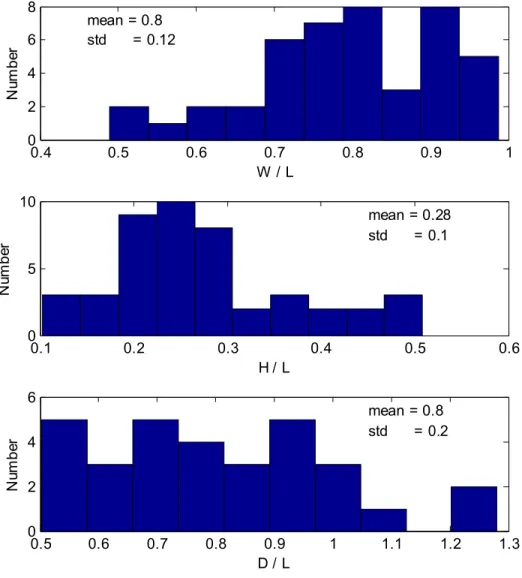
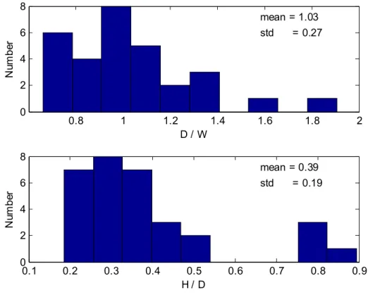
Histograms of the ratios of these dimensions based on measured data from the PERD database (Fleet Technology, 2004) have been plotted in Figure 3.1 and Figure 3.2. Data from 2002 have been excluded since many iceberg dimensions for this year were

incorrectly identified as measured. It is with some caution that these are plotted, since a few of the measurements are clearly inaccurate and some from other years are also estimated, rather than measured. The same histograms are also plotted in Figure 3.3 and Figure 3.4 for the data outlined in Chapter 2, from the Hibernia 1982/4, DIGS and Terra Nova 2003 programs. Data from 231 icebergs were considered in Figure 3.1 and Figure 3.2, while data from 45 icebergs were considered in Figure 3.3 and Figure 3.4. The mean ratios all compare fairly well, indicating that the data used the present report are

representative of the general population of measured icebergs.

Block Coefficients

The block coefficient is the ratio of above water volume to the product of length, width and height, i.e. fVLWH = Va / (LWH). Block coefficients have been derived theoretically for various characteristic shapes, such as wedge, pyramid, dome, tabular and drydock. Historically, these have been used to estimate iceberg mass. Block coefficients were calculated for the Hibernia 1982, DIGS and Terra Nova 2003 data. The calculated values, illustrated in Figure 3.5 and Figure 3.6, demonstrate that there is no difference between the block coefficient for icebergs identified as tabular and other ones, and there is little size influence. The mean block coefficient is 0.22.

The distribution of above water block coefficients is bimodal, as illustrated in Figure 3.5. As shown in Figure 3.6, block coefficients for drydock icebergs are distinctly different, with a mean of 0.16, to those for other icebergs (excluding the tabular one), which have a mean of 0.26.

An analogous block coefficient can be derived for the underwater portion of the iceberg. It can be expressed as the ratio of underwater volume to the product of length, width and draft, i.e. fVLWD = Vu / (LWD). The mean value for the Hibernia 1984, DIGS and Terra Nova 2003 data, based on Figure 3.5 and Figure 3.6, is 1.01, which does not depend on the above water shape designation, nor on waterline length.

3.3

3.4

Centre of Mass Relationships

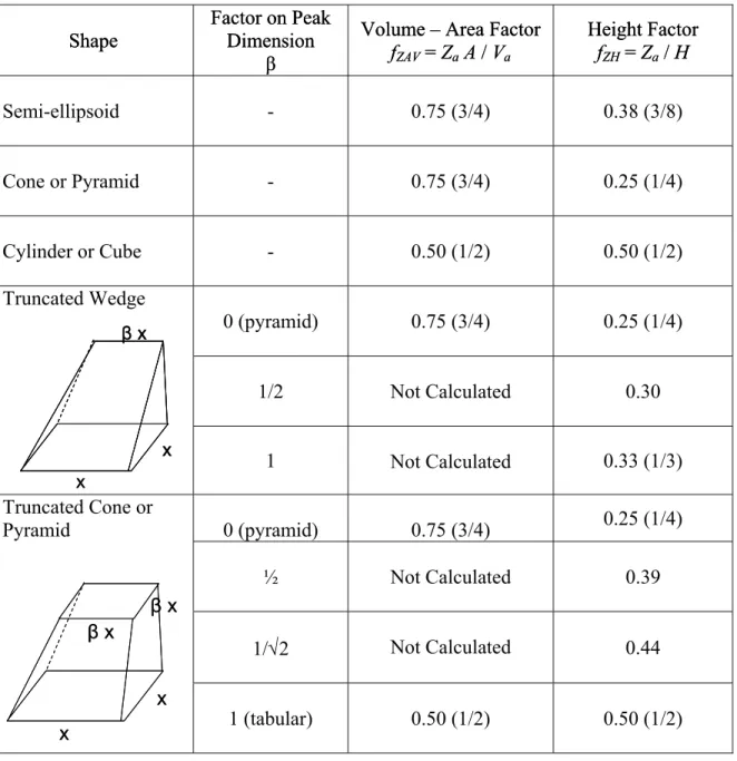
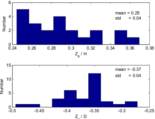
Intuitively, there should be a relationship between the maximum height of an iceberg and the above water centre of mass. The ratio between the centre of mass and maximum height, fZH = Za / H, is shown for a few geometrical shapes in Table 3.1. The distribution of fZH for actual shapes for the Hibernia 1982, DIGS and Terra Nova 2003 data is shown in Figure 3.7. The influence of waterline length on fZH is shown in Figure 3.8. While the relationship is not strong, there may be evidence of a slight increase in fZH with increase in L, which would indicate that larger icebergs are more tabular in shape.

An analogous relationship can also be made between the maximum draft and the

underwater centre of mass. The distribution of the ratio between the centre of mass and maximum draft, fZD = Zu / D, is shown for the Hibernia 1984, DIGS and Terra Nova 2003 data in Figure 3.7. Based on Figure 3.8, there is no influence of waterline length on fZD.

Centre of Mass for Hibernia 1984 Icebergs

For the Hibernia 1984 data set, contours are only available for the underwater portion of the iceberg (Dobrocky Seatech, 1984). When underwater contours only are available, the overall centre of mass can be calculated from

Z = (Za Va + Zu Vu) / V

where Za is the above water centre of mass, Va is above water volume, Zu is the underwater centre of mass, Vu is underwater volume and V is the overall volume. The overall volume is estimated from

V = (ρw / ρi) Vu

where ρw is the water density (1025 kg / m3) and ρi is the ice density (900 kg / m3), and the above water volume is estimated from

Va = (ρw / ρi – 1) Vu

The above water centre of mass is missing in the Hibernia 1984 data and needs to be estimated for use in Section 3.5. A couple of different approaches were investigated. The first was to consider the ratio of above water centre of mass to above water height, i.e.

fZH = Za / H

where H is the iceberg height. The second was to consider the ratio of above water centre of mass times waterline area to the above water volume,

where A is the waterline area.

Each of these indices has been calculated for some characteristic geometric shapes (Table 3.1), for fourteen icebergs from the Hibernia 1982 above water data set (Table 2.1), for six icebergs from the Terra Nova 2003 data set (Table 2.3) and for two icebergs from the DIGS dataset (Table 2.4). The average height ratio from the data is fZH = 0.29 (see Figure 3.7), which places the measured shapes very close to cones or pyramids, but not as

rounded as a semi-ellipsoid. The average measured ratio for fZAV is 0.61, which is somewhere between a cone and a cylinder. The variability in fZAV is about twice that for

fZH, so the height ratio was used to correct the centre of mass for the Hibernia 1984 underwater data.

The underwater contours in the Hibernia 1984 data set do not reach the water surface (see Table 2.2). When calculating underwater volume and centre of mass, the uppermost contour was projected up to the water surface to form a right cylinder with the same shape as the contour. For derivation of parameters associated with the radial

representation in Section 3.5, only data from the actual measured contours were used.

3.5 Radial Representation

3.5.1 General Approach

Each iceberg in Table 2.2, Table 2.3 and Table 2.4 was analyzed using the procedure outlined in Appendix A. Briefly the steps were as follows:

• the overall centre of mass for the Hibernia 1984 data was estimated by finding the centre of mass for the above water portion, then using the parameters derived in Section 3.4 to obtain the overall centre of mass – for the DIGS and Terra Nova 2003 data, the centre of mass was determined by finding the centre of area of each contour, then integrating through the iceberg depth;

• horizontal and vertical angles were calculated for points distributed on the surface of a unit sphere (see Appendix A);

• radii were extended from the iceberg centre of mass for the above angles to intersect the surface of the iceberg;

• spatial correlations, ρ, were calculated for the radii, r, for fifteen angular

separation bins, α, between 0 and π – correlations were calculated for the Hibernia 1984 (except for icebergs 16,18,28), DIGS (icebergs 1&2) and Terra Nova 2003 (NRC icebergs 1-6); and

• the mean radius, r0, and the standard deviation of the radius, σs, were evaluated. 3.5.2 Relationships for Radius

For each iceberg, the mean, r0, and standard deviation, σs, of the 362 radii to the surface points (McKenna, 2004) were calculated. There is a clear relationship between the mean radius and waterline length, i.e. r0 = 0.47 L, as illustrated in Figure 3.9, and deviations about the best fit have a standard deviation of 12 m. The coefficient of variation, σs / r0, has a mean of 0.19 and a standard deviation of 0.06 as shown in Figure 3.10.

The relationship between σs and σe, and the dependence of each of these on waterline length is shown in Figure 3.11. It appears that σe≥ σs in all cases. Were the correlation function a perfect fit, then the two would be equal. Neither σs nor σe depends on iceberg size.

3.5.3 Spatial Correlations

For later use in iceberg generation (Chapter 4), a relationship for spatial correlation as a function of separation angle, α, was developed. A variety of trigonometric and

exponential functions and combinations thereof were investigated, including the function used in McKenna (2004). After some trial and error, the best overall proved to be a quadratic spline between 0 and π/2, and a cubic spline between π/2 and π. These only depended on two parameters: q1, the minimum of the correlation function at α = π/2, and

q2, the value of the correlation function at α = π. The constraints on the splines were ρ(0) = 1, ρ(π/2) = q1, ρ(π) = q2, and dρ/dα(π/2) = dρ/dα(π) = 0. Applying these constraints yielded

ρ = 1 – (4/π) (1 – q1) α + (4/π2) (1 – q1) α 2 ; 0 ≤ α≤ π/2 and

ρ = q2 + 4 (q2 – q1) – (24/π) (q2 – q1) α

+ (36/π2) (q2 – q1) α 2 – (16/π3) (q2 – q1) α 3 ; π/2 < α≤ π

These expressions were fit using a least squares approach simultaneously over the two ranges 0 ≤ α≤ π/2 and π/2 < α≤ π, with the additional constraint q2 > q1, yielding estimates of the parameters q1 and q2.

The individual distributions of the correlation function parameters are given in Figure 3.12. The relationship between q1 and q2 for the different icebergs and their dependence on waterline length is shown in Figure 3.13.

3.5.4 Example Results

To illustrate the procedure, data from a few icebergs have been plotted.

The radial representation for Hibernia 1984 iceberg 35 is shown in Figure 3.14, the distribution of radii is given in Figure 3.15 and Figure 3.16, and the binned correlations and function fit are illustrated in Figure 3.17.

The radial representation for DIGS iceberg 1 is shown in Figure 3.18, the distribution of radii is given in Figure 3.19 and Figure 3.20, and the binned correlations and function fit are illustrated in Figure 3.21.

The radial representation for Terra Nova iceberg 6 is shown in Figure 3.22, the

distribution of radii is given in Figure 3.23 and Figure 3.24, and the binned correlations and function fit are illustrated in Figure 3.25.

For the majority of icebergs, a correlation function that falls off steeply for small separation angles is appropriate. Physically, this means that adjacent points on the iceberg are not correlated exactly and the iceberg surface is rough. Certain icebergs do have portions that are smooth, and the correlation function does not fall off as sharply as the assumed form. A cubic spline with zero slope at α = 0 and cosine forms have been investigated for such cases. Further investigation into the form of the correlation function is recommended.

Table 3.1 Above water shape parameters for characteristic forms Table 3.1 Above water shape parameters for characteristic forms

Shape Shape Factor on Peak Dimension Factor on Peak Dimension β β

Volume – Area Factor Volume – Area Factor

fZAV = Za A / Va Height Factor Height Factor fZH = Za / H f fZAV = Za A / Va ZH = Za / H Semi-ellipsoid - 0.75 (3/4) 0.38 (3/8) Cone or Pyramid - 0.75 (3/4) 0.25 (1/4) Cylinder or Cube - 0.50 (1/2) 0.50 (1/2) 0 (pyramid) 0.75 (3/4) 0.25 (1/4) 1/2 Not Calculated 0.30 Truncated Wedge 1 Not Calculated 0.33 (1/3) 0 (pyramid) 0.75 (3/4) 0.25 (1/4) ½ Not Calculated 0.39 1/√2 Not Calculated 0.44 Truncated Cone or Pyramid 1 (tabular) 0.50 (1/2) 0.50 (1/2) x x β x x x β x x β x x β x β x x x β x β x x

0 0.2 0.4 0.6 0.8 1 0 20 40 60 W / L Nu m b e r mean = 0.72 std = 0.19 0 0.1 0.2 0.3 0.4 0.5 0.6 0.7 0.8 0.9 0 50 100 H / L Nu m b e r mean = 0.23 std = 0.11 0 0.5 1 1.5 2 2.5 3 3.5 4 4.5 0 50 100 150 D / L Nu m b e r mean = 0.79 std = 0.36

Figure 3.1 Histograms for ratio of width, height and draft to waterline length – data from PERD database

0 1 2 3 4 5 6 0 50 100 150 D / W Nu m b e r mean = 1.15 std = 0.65 0 0.2 0.4 0.6 0.8 1 1.2 1.4 0 20 40 60 80 H / D Nu m b e r mean = 0.31 std = 0.14

Figure 3.2 Histograms for ratios of draft to width, and height to draft – data from PERD database

0.4 0.5 0.6 0.7 0.8 0.9 1 0 2 4 6 8 W / L Nu m b e r mean = 0.8 std = 0.12 0.1 0.2 0.3 0.4 0.5 0.6 0 5 10 H / L Nu m b e r mean = 0.28 std = 0.1 0.5 0.6 0.7 0.8 0.9 1 1.1 1.2 1.3 0 2 4 6 D / L Nu m b e r mean = 0.8 std = 0.2

Figure 3.3 Histograms for ratio of width, height and draft to waterline length – Hibernia 1982, Hibernia 1984, DIGS and Terra Nova 2003 data

0.8 1 1.2 1.4 1.6 1.8 2 0 2 4 6 8 D / W Nu m b e r mean = 1.03 std = 0.27 0.1 0.2 0.3 0.4 0.5 0.6 0.7 0.8 0.9 0 2 4 6 8 H / D Nu m b e r mean = 0.39 std = 0.19

Figure 3.4 Histograms for ratios of draft to width, and height to draft –Hibernia 1984, DIGS and Terra Nova 2003 data

0.1 0.15 0.2 0.25 0.3 0.35 0 2 4 6 V_a / L W H Nu m b e r mean = 0.22 std = 0.06 0 0.5 1 1.5 2 2.5 3 0 5 10 15 V_u / L W D Nu m b e r mean = 1.01 std = 0.68

Figure 3.5 Histograms of block coefficients – Hibernia 1982, Hibernia 1984, DIGS and Terra Nova 2003 data

0 50 100 150 200 250 300 0.1 0.15 0.2 0.25 0.3 0.35 V a / L W H tabular drydock (mean=0.16) other (mean=0.26) 0 50 100 150 200 250 300 0 1 2 3 V u / L W D L [m] tabular non-tabular

Figure 3.6 Relationship between block coefficient and waterline length – Hibernia 1982, Hibernia 1984, DIGS and Terra Nova 2003 data

0.240 0.26 0.28 0.3 0.32 0.34 0.36 0.38 2 4 6 Z_a / H Nu m b e r mean = 0.29_{std = 0.04} -0.50 -0.45 -0.4 -0.35 -0.3 -0.25 5 10 15 Z_u / D Nu m b e r mean = -0.37 std = 0.04

Figure 3.7 Histograms for ratio of above and below water centres of mass to height and draft – Hibernia 1982, Hibernia 1984, DIGS and Terra Nova 2003 data

0 50 100 150 200 250 300 0.2 0.25 0.3 0.35 0.4 Z a / H tabular non-tabular 0 50 100 150 200 250 300 -0.5 -0.45 -0.4 -0.35 -0.3 -0.25 L [m] Z u / D

0 20 40 60 80 100 120 140 0 20 40 60 80 L [m] r 0 [m ] tabular non-tabular r₀ = 0.47 L -20 -15 -10 -5 0 5 10 15 20 25 0 2 4 6 8 mean = 2.05 std = 11.84 r₀ - 0.47 L Nu m b e r

Figure 3.9 Relationship between mean radius and waterline length – Hibernia 1984, DIGS and Terra Nova 2003 data

0.1 0.15 0.2 0.25 0.3 0.35 0 2 4 6 8 mean = 0.19 std = 0.06 σ_s / r ₀ Nu m b e r 0 0.2 0.4 0.6 0.8 1 1.2 1.4 0 5 10 15 20 mean = 0.25 std = 0.21 σ_e / r ₀ Nu m b e r

Figure 3.10 Histograms of coefficients of variation for deviations from mean radius and residual from radial fit – Hibernia 1984, DIGS and Terra Nova 2003 data

0 50 100 150 200 250 300 0 10 20 30 σ s tabular non-tabular 0 50 100 150 200 250 300 0 20 40 60 σ e L [m] 0 5 10 15 20 25 0 20 40 60 σ _s σ e

Figure 3.11 Scatter plots for average values of deviations from mean radius and residual from radial fit – Hibernia 1984, DIGS and Terra Nova 2003 data

-0.40 -0.35 -0.3 -0.25 -0.2 -0.15 2 4 6 8 mean = -0.23 std = 0.08 q₁ Nu m b e r -0.20 0 0.2 0.4 0.6 0.8 2 4 6 mean = 0.26 std = 0.26 q₂ Nu m b e r

Figure 3.12 Distributions of correlation parameters – Hibernia 1984, DIGS and Terra Nova 2003 data

0 50 100 150 200 250 300 -0.5 0 0.5 1 L [m] C o rre la ti o n P a ra m e te r q₁ tabular q₁ non-tabular q₂ tabular q₂ non-tabular -0.2 0 0.2 0.4 0.6 0.8 -0.4 -0.3 -0.2 -0.1 0 q₂ q 1 tabular non-tabular q₁ = - 0.18 - 0.21 q ₂ -0.10 -0.05 0 0.05 0.1 0.15 2 4 6 mean = 0 std = 0.05 Residual = q₂ + 0.18 + 0.21 q ₁ Nu m b e r

Figure 3.13 Correlation parameter relationships – Hibernia 1984, DIGS and Terra Nova 2003 data

-20 0 20 -20 0 20 -60 -50 -40 -30 -20 -10 Hibernia 1984 Iceberg 35

Figure 3.14 Radial representation for Hibernia 1984 iceberg 35

15 20 25 30 35 40 45 0 20 40 60 80

Radius to Iceberg Surface [m]

Nu m b e r Hibernia 1984 Iceberg 35 -10 -5 0 5 10 15 0 20 40 60 80

Deviation from Mean Radius [m]

Nu

m

b

e

r

Figure 3.15 Distribution of radius and deviations from mean radius for Hibernia 1984 iceberg 35

-40 -30 -20 -10 0 10 20 30 0 50 100 150 Nu m b e r -30 -20 -10 0 10 20 0.001 0.003 0.01 0.02 0.05 0.10 0.25 0.50 0.75 Residual [m] P ro bab il it y Data Normal Distribution

Figure 3.16 Distribution of residual from radial representation for Hibernia 1984 iceberg 35 0 20 40 60 80 100 120 140 160 180 -0.2 0 0.2 0.4 0.6 0.8 1 1.2 Angular Separation [o] Co rr e la ti o n C o e ffi ci e n t Hibernia 1984 Iceberg 35

-50 0 50 -50 0 50 -100 -80 -60 -40 -20 0 20 DIGS Iceberg 1

Figure 3.18 Radial representation for DIGS iceberg 1

40 50 60 70 80 90 100 110 0 20 40 60 80

Radius to Iceberg Surface [m]

Nu m b e r DIGS Iceberg 1 -30 -20 -10 0 10 20 30 40 0 20 40 60 80

Deviation from Mean Radius [m]

Nu

m

b

e

r

Figure 3.19 Distribution of radius and deviations from mean radius for DIGS iceberg 1

-40 -30 -20 -10 0 10 20 30 40 0 50 100 150 Nu m b e r DIGS Iceberg 1 -40 -30 -20 -10 0 10 20 30 40 0.001 0.003 0.01 0.02 0.05 0.10 0.25 0.50 0.75 Residual [m] P robab il it y Data Normal Distribution

Figure 3.20 Distribution of residual from radial representation for DIGS iceberg 1

0 20 40 60 80 100 120 140 160 180 -0.4 -0.2 0 0.2 0.4 0.6 0.8 1 Angular Separation [o] C o rr e la ti o n C o e ffi ci e n t DIGS Iceberg 1

-20 0 20 -40 -20 0 20 40 -60 -40 -20 0 20

Terra Nova 2003 Iceberg 6

Figure 3.22 Radial representation for Terra Nova 2003 iceberg 6

20 25 30 35 40 45 50 55 60 0 20 40 60 80

Radius to Iceberg Surface [m]

Nu

m

b

e

r

Terra Nova 2003 Iceberg 6

-20 -15 -10 -5 0 5 10 15 20 0 20 40 60 80

Deviation from Mean Radius [m]

Nu

m

b

e

r

Figure 3.23 Distribution of radius and deviations from mean radius for Terra Nova 2003 iceberg 6

-30 -20 -10 0 10 20 30 0 50 100 150 Nu m b e r

Terra Nova 2003 Iceberg 6

-20 -15 -10 -5 0 5 10 15 20 0.001 0.003 0.01 0.02 0.05 0.10 0.25 0.50 0.75 Residual [m] P robab il it y Data Normal Distribution

Figure 3.24 Distribution of residual from radial representation for Terra Nova 2003 iceberg 6 0 20 40 60 80 100 120 140 160 180 -0.2 0 0.2 0.4 0.6 0.8 1 Angular Separation [o] C o rr el at ion C o ef fi ci ent

Terra Nova 2003 Iceberg 6

4 ICEBERG GENERATION

4.1 Iceberg Generation

The statistical model developed in CHC/PERD Report 20-73 was used to generate a number of representative iceberg shapes. A full description, with minor changes, is included in Appendix A. Initially, it was anticipated that a more exact procedure would be used to determine equilibrium positions for the generated iceberg shapes. This approach has not yet been integrated and the approximate procedure developed in CHC/PERD Report 20-73 (also outlined in Appendix A) was used instead. The iceberg generation procedure is as follows:

• a unit radius, r0, was selected;

• the random deviations were sampled from a normal distribution with σe = r0 N(0.19,0.04), based on the distribution of s in Figure 3.10;

• the correlation parameter q2 was sampled from the uniform distribution U(-0.2,0.8), based on Figure 3.13;

• the correlation parameter q1 was sampled from -0.18 - 0.21q2 + N(0,0.05), from Figure 3.13;

• the correlation matrix, R, was generated from q1 and q2, and the angles to points on the unit sphere;

• the B matrix was obtained as the matrix square root of R (using the MATLAB sqrtm function);

• the iceberg shape was generated from the radii r = r0 + B e;

• icebergs were rejected unless the centre of mass was within a prescribed tolerance according to the procedure described in Appendix A; and

• the iceberg orientation and depth were calculated using the algorithm outlined in Appendix A.

The above procedure produces icebergs with unit mean radius that can be scaled geometrically. If actual iceberg sizes are required, it is recommended that waterline length, L, be sampled from an appropriate distribution for the region under consideration. The mean iceberg radius can then be sampled from r0 = L [0.47 + N(0,12)], according to Figure 3.9.

All of the above sampling relationships were derived from the Hibernia 1984, DIGS and Terra Nova 2003 data, as outlined in Chapter 3.

A few icebergs generated using the above procedure are shown in Figure 4.1 through Figure 4.4. While these icebergs are realistic, they are generally quite angular and may not capture some of the smoother forms in the observed icebergs. The iceberg shape is largely driven by the form of the correlation function and the present characterization may be somewhat restrictive. Aside from the present one, there exist numerous other ways of generating random surfaces. In future, it is recommended that these be investigated.

Symmetric positive definite forms of the matrix R result from some simple geometries and parameters q1 and q2, in which case Cholesky factorization can be used to calculate B. In this case, B is always real and the solution is straightforward. For the large majority of cases, R is symmetric but not positive definite. In such cases, for certain values of the correlation function parameters q1 and q2, the matrix B is complex, implying there is no real matrix for the square root of R. When this occurred, the magnitude of the complex vector s = B e was used to generate the iceberg radii. In future, the investigation of other forms for the correlation function is recommended, since these may potentially lead to better forms for the correlation matrix, R.

4.2 Validation of Index Dimensions and Measured Relationships

Index dimensions, consisting of waterline length, L, waterline width, W, maximum height, H, and maximum draft, D, were calculated for each of 500 generated icebergs. The total volume, and the portions above and below water were also calculated. Ratios between the index dimensions and the block coefficients for the generated icebergs are shown in Figure 4.5, Figure 4.6 and Figure 4.7.

These can be compared to those from the icebergs used to develop the radial shape relationships (previously shown in Figure 3.3, Figure 3.4 and Figure 3.5) and for other icebergs in PERD databases (previously shown in Figure 3.1 and Figure 3.2). A comparison of means and standard deviations for the ratios is shown in Table 4.1. Overall, the ratios of index dimensions for the generated icebergs compare favourably with those from the data. The average width to length ratio is consistent with the data, the height to length ratio is slightly lower, while the draft to length ratio is higher. The height to draft ratio is lower, while the draft to width ratio is consistent with the data. An ice density of 890 kg/m3 and a water density of 1025 kg/m3 were assumed for

determining the waterline of the generated icebergs. A lower value for the assumed ice density could potentially bring the average generated ratio in line with measured values. The standard deviations of the ratios for the generated icebergs are consistently lower than for the data, indicating that the variability in shape is not captured entirely by the statistical representation. The parametrization of the correlation function is probably the cause.

The average above water block coefficient, Va / (LWH), for generated icebergs is consistent with the measured value and its variability is similar. For the underwater block coefficient, Vu / (LWD), the generated value is significantly less than for the data. The data are dominated by icebergs from the Hibernia 1984 program, in which the underwater volumes were estimated by projecting the highest contour to the water surface. This most probably led to an overestimation in the underwater volume, thereby explaining some of the discrepancy.

Table 4.1 Comparison of characteristic ratios from the PERD database, from Hibernia 1982, Hibernia 1984, DIGS and Terra Nova 2003 data, and from generated icebergs

Based on PERD Database

Based on Data Used for Shape Characterization

Generated Characteristic

Ratio

Mean Std. Dev. Mean Std. Dev. Mean Std. Dev.

W / L 0.79 0.19 0.80 0.12 0.81 0.11 H / L 0.23 0.11 0.28 0.10 0.21 0.05 D / L 0.79 0.36 0.80 0.20 0.84 0.09 D / W 1.15 0.65 1.03 0.27 1.05 0.l3 H / D 0.31 0.14 0.39 0.19 0.24 0.05 Va / (LWH) - - 0.22 0.06 0.20 0.10 Vu / (LWD) - - 1.01 0.68 0.68 0.15

Figure 4.1 Radial representation for generated iceberg A

Figure 4.3 Radial representation for generated iceberg C

0.4 0.5 0.6 0.7 0.8 0.9 1 0 50 100 150 W / L mean = 0.81 std = 0.11 0.050 0.1 0.15 0.2 0.25 0.3 0.35 0.4 0.45 100 200 H / L mean = 0.21 std = 0.05 0.5 0.6 0.7 0.8 0.9 1 1.1 1.2 0 50 100 150 D / L mean = 0.84 std = 0.09

Figure 4.5 Histograms of ratio of width, height and draft to waterline length for generated icebergs

0.8 1 1.2 1.4 1.6 1.8 2 0 50 100 150 D / W mean = 1.05 std = 0.13 0.1 0.15 0.2 0.25 0.3 0.35 0.4 0.45 0.5 0 50 100 150 H / D mean = 0.24 std = 0.05

Figure 4.6 Histograms of ratios of draft to width, and height to draft for generated icebergs 0.050 0.1 0.15 0.2 0.25 0.3 0.35 0.4 0.45 0.5 50 100 150 V_a / (L W H) mean = 0.2 std = 0.1 0.2 0.4 0.6 0.8 1 1.2 1.4 1.6 0 50 100 150 200 V_u / (L W D) mean = 0.68 std = 0.14

5 CONCLUSIONS AND RECOMMENDATIONS 5.1

5.2

Conclusions

Tabular icebergs, and particularly those from certain glaciers, are clearly different in shape than the general iceberg population. Unfortunately, these were not well

represented in the Hibernia 1982, Hibernia 1984, DIGS and Terra Nova 2003 data under consideration. Based on the present analysis, there is little reason to differentiate data from tabular and other iceberg shapes.

Block coefficients for the drydock icebergs analyzed, with a mean of 0.16, are clearly less than those with other shape designations, which have a mean of 0.26. There were insufficient tabular icebergs in the dataset to make any conclusions in this regard. These is little effect of iceberg size, as represented by waterline length, on any of the indices of iceberg shape considered in this report. Based on data from the Hibernia 1982, Hibernia 1984, DIGS and Terra Nova 2003 programs, there is justification for the

consideration of geometrically similar iceberg shapes that can be scaled by the waterline length. Clearly, there exist size effects on iceberg shape, particularly when dealing with very large or tabular icebergs, but these are not in evidence from the data considered. The icebergs generated using the procedure developed in McKenna (2004) and refined in this report provide a good representation of global iceberg shape, as demonstrated

through a comparison with measured ratios of index dimensions and block coefficients. For above water geometry, the multiple scaled digital photos of the skyline profile used in the Terra Nova 2003 program appear to yield accurate data.

Recommendations

The present iceberg shape characterization is based on 28 icebergs from the Hibernia 1984, DIGS and Terra Nova 2003 programs. Many other data exist that could potentially be included, such as the third iceberg from the DIGS program, approximately 50 icebergs from Terra Nova and White Rose sponsored programs in 2002, 2003 and 2004, and from upwards of 600 above water geometries acquired during the Hibernia development process. There also exist many 2D underwater and above water profiles that could be used with suitable estimation of the location for centre of mass.

The present radial shape characterization does not distinguish between the various iceberg shapes. When additional data are considered, it may be possible to differentiate the shape parameters based on the standard shape designations – tabular, dome, drydock, pinnacle and wedge.

Aside from the present one, which is conceptually fairly simple, there exist numerous other approaches for generating random surfaces. In future, it is recommended that some of these be investigated.

Correlations between surface points distributed about the iceberg have been represented using a two parameter function. This may be restrictive and further investigation into the form of the function is recommended.

Focus in this report has been on global iceberg shape. Much of the present approach can also be applied to local shape, which is key for establishing the relationship between nominal contact area and penetration used in iceberg load analysis. Above water data from the 1982, 1983 and 1984 Hibernia programs, from the 2002 and 2003 Terra Nova programs and from the 2004 White Rose program could be used for this purpose if deemed to be representative of underwater shape. For the underwater measurements, 3D geometry from the 1984 Hibernia program appears to be the best. If 2D profile data can be used, a number of other programs may be appropriate.

Underwater iceberg geometry is difficult to measure accurately. Experience with the interpretation of data from each of the programs considered in this report has

demonstrated some inadequacies. For example, there are creases in the Terra Nova 2003 contours at the base of the keel, which is likely caused by differential drift of the sonar head with respect to the vessel. To ensure accuracy in the measurement of keel

geometry, redundant strategies could potentially be used in future. The Hibernia 1984 contours do not reach the water surface, nor do they always reach the deepest part of the keel.

In the PERD shape database (Canatec et al., 1999), iceberg contour data are included without discrimination of multiple contour segments at each level. Many potential uses of the data require this information. When multiple contour segments are present at a given elevation, the segments need to be associated with the ones immediately above and below. Efficient formatting requires a hierarchical reference system for the different contour segments and the identification of whether a contour represents a trough or a peak. If future initiatives are made on the shape database, a proper reference system is recommended.

Some of the iceberg geometries analyzed do not appear to be stable hydrostatically. This is not unexpected, since icebergs are in a state of decay and may only be marginally stable. Even relatively small errors in the measurement of a portion of the keel could contribute to apparent instability. A thorough investigation of the stability of the icebergs documented in this report is recommended. For the Hibernia 1984 data, where only the underwater portion has been profiled, stability limits could help to specify more accurate above water centre of mass.

Focus in this report has been on only a few key shape relationships. There exist numerous others, including stability, depth associated with maximum width, and projected areas that should also be considered.

The ultimate objective of a statistical representation for iceberg shape is to generate large numbers of representative icebergs that can be used for risk and impact load calculations

for offshore installations. At present, there are less than 100 full measured iceberg profiles in existence. Many are inaccurate, are missing significant portions and are not stable hydrostatically. Generated icebergs would have a smooth transition through the waterline, which cannot be measured using present techniques, and would not suffer from degradation in accuracy at the base of the keel. The present approach is close to

achieving this goal, but requires a more robust formulation and consideration of all measured iceberg data where the centre of mass is known or can be inferred.

6 REFERENCES

Atlantic Survey (1982) Iceberg aerial reconnaissance, Atlantic Survey report for Mobil Hibernia Development Studies.

Bercha (1983) Iceberg aerial reconnaissance 1983, F.G. Bercha and Associates report for Mobil Hibernia Development Studies.

Bercha (1984) Iceberg aerial reconnaissance 1984, F.G. Bercha and Associates report for Mobil Hibernia Development Studies.

Canatec et al. (1999) Compilation of iceberg shape and geometry data for the Grand Banks region, PERD/CHC Report 20-43 by CANATEC Consultants Ltd., ICL Isometrics Ltd., CORETEC Inc. and Westmar Consultants Ltd.

Dobrocky Seatech (1984) Iceberg field survey 1984. Mobil Hibernia Development Studies.

Fleet Technology (2004) PERD iceberg sighting database: 2004, Fleet Technology report to Canadian Hydraulics Centre, PERD/CHC Report 20-86.

Hodgson, G.J., Lever, J.H., Woodworth-Lynas, C.M., Lewis, C.F. (1988) The dynamics of iceberg grounding and scouring (DIGS) experiment and repetitive mapping of the eastern Canadian continental shelf, ESRF Report No.094.

Intera (1981) Iceberg dimensions by aerial photography. Intera Environmental Consultants Ltd., Report for Mobil Hibernia Development Studies.

McKenna, R.F. (2004) Iceberg shape characterization for risk to Grand Banks structures, PERD/CHC Report 20-73 by Richard McKenna.

McKenna, R.F. (2005) Iceberg shape characterization, in proceedings of POAC’05 Conference, Potsdam, New York.

Oceans Ltd. (2004) Determination of Iceberg Draft and Shape. PERD/CHC Report 20-75 by Oceans Ltd..

A STATISTICAL REPRESENTATION OF ICEBERG SHAPE

A.1 Basic Theory

An approach was developed in McKenna (2004) for the characterization of three dimensional iceberg shape in terms of the overall average shape and random deviations about the average. The present derivation follows this approach closely, with some minor cosmetic changes. The theory is based on the principles of spatial statistics, considering deviations from the average shape as shown in Figure A.1. These deviations are assumed to be randomly distributed about 0 and only depend on the distance between them, with the distribution dictated by measured iceberg shapes. For a spherical average shape, the distance between surface points can be represented in terms of angular

separations as shown in Figure A.1.

A.2 Spherical Geometry

The spherical mean shape with radius r0 is illustrated in Figure A.2. Two surface points with indices i, j are shown, along with corresponding horizontal angles θi, θj and vertical angles φi, φj. The angular separation between the two surface points is αij.

The coordinates of the surface point with radius ri are

xi = ri cosθi cosφj.= ri f(θi, φi) [Eq. A.1]

yi = ri sinθi cosφj.= ri g(θi, φi) [Eq. A.2] and

zi = ri sinφj.= ri h(θi, φi) [Eq. A.3] The surface of the sphere is represented by a large number of distinct points and each is associated with a surface area as shown in Figure A.3. In practice, the points are

distributed evenly around the surface of the sphere such that the incremental surface areas are approximately equal. The size of the incremental surface area is

ai = qi ri2 [Eq. A.4]

where qi is a constant that depends on the choice for the layout of the surface points. The elemental volume is approximately

vi = (1/3) qi ri3 [Eq.A.5]

and its centre of mass is located a distance of approximately