Paleoclimatic reconstructions in western Canada from boreholetemperature logs: surface air temperature forcing and groundwater flow

HAL Id: hal-00298039

https://hal.archives-ouvertes.fr/hal-00298039

Submitted on 14 Feb 2006

HAL is a multi-disciplinary open access

archive for the deposit and dissemination of

sci-entific research documents, whether they are

pub-lished or not. The documents may come from

teaching and research institutions in France or

abroad, or from public or private research centers.

L’archive ouverte pluridisciplinaire HAL, est

destinée au dépôt et à la diffusion de documents

scientifiques de niveau recherche, publiés ou non,

émanant des établissements d’enseignement et de

recherche français ou étrangers, des laboratoires

publics ou privés.

boreholetemperature logs: surface air temperature

forcing and groundwater flow

J. Majorowicz, S. E. Grasby, G. Ferguson, J. Safanda, W. Skinner

To cite this version:

J. Majorowicz, S. E. Grasby, G. Ferguson, J. Safanda, W. Skinner. Paleoclimatic reconstructions

in western Canada from boreholetemperature logs: surface air temperature forcing and groundwater

flow. Climate of the Past, European Geosciences Union (EGU), 2006, 2 (1), pp.1-10. �hal-00298039�

Climate of the Past, 2, 1–10, 2006 www.climate-of-the-past.net/cp/2/1/ SRef-ID: 1814-9332/cp/2006-2-1 European Geosciences Union

Climate

of the Past

Paleoclimatic reconstructions in western Canada from borehole

temperature logs: surface air temperature forcing and groundwater

flow

J. Majorowicz1,2, S. E. Grasby3, G. Ferguson4, J. Safanda5, and W. Skinner6

1_{Northern Geothermal, 105 Carlson Close, Edmonton, Alberta, T6R 2J8, Canada}

2_{University of North Dakota, Northern Plains Climate Research Centre, Grand Forks, USA} 3_{Geological Survey of Canada, Calgary, Canada}

4_{Department of Earth Sciences, St. Francis Xavier University, Antigonish, Nova Scotia, Canada} 5_{Geophysical Institute, Prague, Czech Republic}

6_{Environment Canada, Downsview, Ont., Canada}

Received: 15 June 2005 – Published in Climate of the Past Discussions: 9 August 2005 Revised: 2 November 2005 – Accepted: 11 January 2006 – Published: 14 February 2006

Abstract. Modelling of surface temperature change effect on temperature vs. depth and temperature-depth logs in West-ern Canada Sedimentary Basin show that SAT (surface air temperature) forcing is the main driving factor for the under-ground temperature changes diffusing with depth. It supports the validity of the basic hypothesis of borehole temperature paleoclimatology, namely that the ground surface tempera-ture is systematically coupled with the air temperatempera-ture in the longer term (decades, centuries). While the highest ground-water recharge rate used in the modelling suggests that for this extreme case some of the observed curvature in the pro-file, could be due to groundwater flow, it is more likely that the low recharge rates in this semi-arid region would have minimal impact. We conclude that surface temperature forc-ing is responsible for most of the observed anomalous tem-perature profile.

1 Introduction

The primary assumption of borehole paleoclimatology (Lachenbruch, 1994) is that heat transfer is by conduction only. This assumption is justified in areas with negligible vertical movement of subsurface water (Kane et al., 2001). Groundwater flow is often neglected in GST (ground surface temperature) reconstructions without adequate justification according to recent studies of Reiter (2005) and Ferguson and Woodbury (2005).

If the observed temperature logs can be explained assuming only conductive heat transport on the multi-decadal/century time scale, GST histories derived from well

Correspondence to: J. Majorowicz

(majorowicz@shaw.ca)

temperatures over the past several centuries may be much more believable. We can test the above assumption by com-paring measured transient temperature – depth profiles (T-z) with simulated profiles from the surface air temperature SAT data of nearby climate stations.

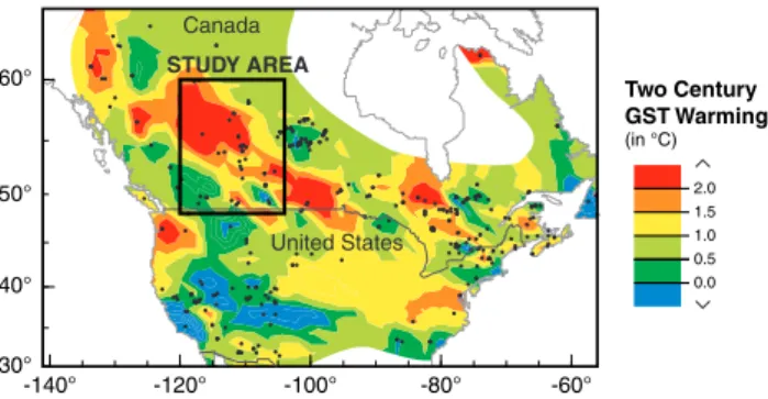
In this paper we report results of temperature (T) mea-surements with depth (z) for borehole sites located in the Western Canadian Sedimentary basin, with special focus on the Paskapoo Formation in western Alberta. The Mid-west of North America (northern Great Plains in the USA and Western Canadian Prairies) has been experiencing one of the highest mean annual surface air and ground warming in the Northern Hemisphere (Skinner and Majorowicz, 1999; Gos-nold et al., 1997), characterized by a GST warming magni-tude of +2.1◦C +/−1◦C over some two centuries (Fig. 1).

2 Theory

The past changes in the energy balance at the Earth’s surface propagate into the subsurface and appear as perturbations of the subsurface thermal regime. Due to the low thermal dif-fusivity of rocks, GST changes propagate downward slowly and are recorded as transient perturbations to the steady state temperature field. Temperature profiles measured in a bore-hole a few hundred metres deep may contain information about GST changes in the last millennium. This gives us an opportunity to reconstruct surface temperature history by in-version of the temperature T vs. depth z profile T(z). The re-sult is considered to be a climate record with a secular length proportional to depth of the borehole temperature measure-ment.

The reconstruction of the GST history is done for time in-terval [t0–t1] from the subsurface temperature profile T(z, t1)

60° 40° 30° 50° -140° -120° -100° -80° -60° Canada STUDY AREA United States Two Century GST Warming (in °C) 0.0 1.0 0.5 1.5 2.0

Fig. 1. The location of the study area (within Western

Cana-dian Sedimentary basin in Alberta and Saskatchewan) is shown against the map of latest warming/cooling amplitude within the last 200 years from well temperature data location of which is shown by black dots. This amplitude was determined using a priori “ramp” model described in Lachenbruch (1994). Study area is well within high warming area called here MWWA (mid-west warming anomaly). Contours are in degrees C.

measured between the surface and depth zbat time t1. It im-plicitly requires that the perturbations in T(z,t) caused by the GST variation before time t0 cannot be distinguished from the steady-state field within the depth interval [0, zb] at time t1. This requirement can be satisfied by considering t0 suffi-ciently far away from t1.

The GST change will produce a disturbance to an other-wise linear portion of the well temperature profile assuming constant conductivity K and diffusivity a. The linear portion of the well temperature profile represents steady flow of heat Q from the earth’s interior according to Fourier relation:

Q = −kGo (1)

Where k is thermal conductivity and Gois thermal gradient. Extrapolation of the linear portion of thermal profile con-trolled by deep heat flow Qand thermal conductivity k to the surface zo yields the intercept temperature T (zo). The deviation of the measured temperature profile T (z)from the extrapolated linear profile results in temperature anomaly

1T(z), which in the simplest interpretation represents the

response of the ground to recent rise of the mean annual surface temperature from a previous long-term value T (zo) (positive anomaly values) or recent cooling (in case of nega-tive anomaly). The combination of subsequent warming and cooling events complicates the disturbing signal with depth.

Heterogeneities in rock properties and three-dimensional effects limit resolution of the details of T (z, t), where t is time, however, a one dimensional model is capable of resolv-ing the general magnitude of recent temperature changes and timing of its onset. In the simple one-dimensional transient model of the effects of surface GST change upon temperature depth, the assumption of homogenous sub-surface media is a

simplification. Temperature change with depth and time can be written as:

T (z, t ) = T (zo) + Goz + 1T (z, t ) (2) where 1T(z, t) represents the response of the ground to re-cent mean annual warming or cooling of the surface from the previous long term value T (zo), and 1T (z,t) is governed by the differential equation

d21T (z, t )/dz2=1/κdT /dt (3) where κ=k/ ρ c is thermal diffusivity, ρ is density and c is heat capacity.

We can simulate the transient subsurface temperature changes caused by the ground surface temperature varia-tions by using the SAT series under the assumption that the mean difference between the ground and air tempera-tures is constant through time. We consider annual means

Tiof the SAT as a ground surface forcing function. POM (pre-observational mean) surface temperature needs to be as-sumed.

The forcing function consisted of a series of N jumps of amplitude 1Ti=Ti−Ti−1at times tibefore the borehole tem-perature measurement. The subsurface temtem-perature response

Tto this forcing at depth z was (Carslaw and Jaeger, 1959)

T (z) = X

i=1−N

1Ti×erf c(z/

√

4κti) (4)

Where, κ is thermal diffusivity and erfc is the complemen-tary error function. This calculation depends on one free pa-rameter, the mean long-term temperature Tobefore the first change at time t1. Parameter Tois the pre-observational mean (POM).

In general, mean annual ground surface temperature tracks the mean annual surface air temperatures taken at screen height (1.5 m above the surface of the ground), on the long scale (Baker and Ruschy, 1993; Putnam and Chapman, 1996, and Majorowicz and Skinner, 1997). However, this rela-tion between ground surface temperature (GST) warming re-constructed from borehole T-z profiles and surface air tem-perature (SAT) warming has been questioned by Mann and Schmidt (2003). Mann and Schmidt (2003) argue that the ground does not “see” much of the cold winter air cooling in the presence of snow cover because of insulation and re-flection of incoming radiation, resulting in potential loss of information of cold-season temperature variations in the re-constructed GST history. Annual means derived from GST are usually higher than the ones from SAT,as the snow cover reduces the heat loss (Lachenbruch, 1994; Schmidt et al., 2001; Stieglitz et al., 2003). The magnitude of the differ-ence between the mean annual ground surface and surface air temperatures depends on snow cover or the content of soil moisture at the beginning of the freezing season. As-suming that departures between ground and air temperatures change randomly from year to year and their mean values do

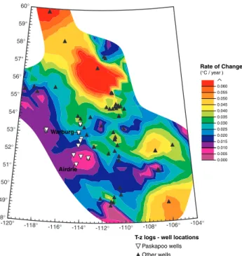
J. Majorowicz et al.: Paleoclimatic reconstructions in western Canada 3 0.005 0.000 0.015 0.010 0.020 0.025 0.030 0.035 0.040 0.045 0.050 0.055 0.060 Rate of Change (°C / year ) Airdrie Warburg

T-z logs - well locations

Paskapoo wells Other wells -120° _{-118° -116°} -114° -112° -110° -108° -106° -104° 60° 59° 58° 57° 56° 55° 54° 53° 52° 51° 50° 49° 48°

Fig. 2. Rate of temperature change for the 1920–1990 A.D. cal-culated from 51 temperature logs in Alberta and S. Saskatchewan using functional space inversion of Shen and Beck (1991).

not change on the time scale of the GST history reconstruc-tion, then the present interpretation of the GST history as a first order estimate of the air temperature history is correct (Putnam and Chapman, 1996; Cermak et al., 2003, Beltrami, 2001; Schmidt et al., 2001; Gonzalez-Rouco et al., 2003). Modelling done by Gonzalez-Rouco et al. (2003) shows that at long time scales terrestrial deep annual soil temperature changes are a good proxy for annual surface air temperature (SAT), and their variations are almost indistinguishable from each other.

Factors like deforestation or forest fires can also sig-nificantly change surface temperature and influence under-ground temperature regimes (Majorowicz and Skinner, 1997; Lewis and Skinner, 2003; Skinner and Majorowicz, 1999). Such changes of the land surface are sometimes not well known and their contribution to the warming/cooling of the surface are not easily separated from the irradiative forcing. In most cases the information about the location of the well and analysis of history of land use in the area can be used to eliminate unwanted logs. Similar to the influence of ground-water flow upon T-z, these effects are difficult to separate from the effects of surface warming on T-z curvature (Reiter, 2005; Ferguson and Woodbury, 2005). All of these (surface warming due to climatic change, changes related to land use, hydrodynamic effects etc.) can influence the behavior of sub-surface temperatures. Depth (m) 4 5 2 3 6 7 8 9 10 11 Temperature (°C) 0 50 100 150 200 1 - Sundre 2 - Airdrie (water filled) 3 - Olds 4 - Warburg 5 - Gull Lake 5 4 3 1 1' _2' 3' _4' 5' 6' 2 2004 Data 1' - Treecreek Basin #50)bs#4 2' - Treecreek Basin 7b 3' - Sylvan Lake 4' - Three Hills RCA144 5' - Hubbles Lake 1922E 6' - Crestomere lake N-Obs1

1992 Data

Fig. 3. Temperature logs in Paskapoo Fm area in Alberta. Logs

done in 1992 are marked by numbers with mark, such as 10;20. . . ;

2004 logs are marked by numbers only, such as 1,2,. . . .

3 Temperature-depth and surface air temperature (SAT) data

Temperature logs were taken in 51 wells through the prairies (Fig. 2) using portable logging equipment with a thermistor probe. The location of wells logged within the Paskapoo area is shown in Fig. 2. Paskapoo well logs are shown in Fig. 3. Locations of other wells with temperature logs are also shown in Fig. 2. Temperature measurements were made be-tween 1991–1995 and as recently as 2004 .The temperature-depth data were used to infer magnitude of recent ground surface temperature (GST) warming (1920–1990 A.D) using the approach described in Majorowicz et al. (2002).

Temperature measurements were made with a thermistor probe calibrated to 0.01◦_{C (relative change) and 0.03}◦_C (ab-solute value). The probe was attached to 500 m cable on a portable, manually operated winch. The measurements were taken at discrete intervals (2 m and 5 m for the oldest log) in observational wells with no disturbances for decades. These wells monitor piezometric water levels only and no other ac-tivities are known after well drilling ceased (before 1980). This ensures that thermal equilibrium exists between water in the well and the surrounding rock mass. Usually, logging of temperature started at depths below 20 m, depending on the static water level on the wells. In some cases, however, measurements were available at shallower depths (Fig. 3). Above 15–20 m, daily to seasonal temperature changes in-fluence soil temperatures in the immediate vicinity of the borehole. That upper part of the cased well above the wa-ter table is filled with air. The small diamewa-ter of the wells relative to their length disallowed any convection in the well bore significant enough to disturb the thermal regime (Jes-sop, 1990). Nevertheless, circulation in an air column likely exists. Our experience based on logging and data analysis shows that it can interact by changing the top few meters of a well’s water column and influence temperature in the very upper few meters of the log (due to induced circula-tion). Variations of static water level (piezometric surface

1900 1920 1940 1960 1980 2000 -2.0 -1.0 0.0 1.0 2.0 3.0 4.0 5.0 6.0 D eg re es C el si u s Graph 1 Annual average Line/Scatter Plot 28

Calmar (3011120) Annual Temperature

Fig. 4. Mean annual surface temperature time series in Calmar En-vironment Canada observational station. Decadal means are also given.

variations) are constantly occurring and can be several me-ters seasonally..These depend on several factors like strong correlation with precipitation, surface temperature changes (drying when hot), on-surface vegetation and changes in recharge.

Rock chip and well log derived net rock lithology and rock conductivities of the Western Canadian Sedimentary Basin (Beach et al., 1987; Jessop, 1990) were used in thermal con-ductivity estimate. Details of concon-ductivity variation with depth were shown in Majorowicz et al. (1999).

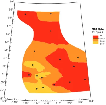
Meteorological data (SAT series) like the one illustrated in Fig. 4, from 22 Environment Canada SAT stations, were used in calculations of SAT warming rates for the 1920– 1990 AD (Fig. 5). These are much less variable than the GST rates calculated from well temperature logs (Fig. 2). However, a trend of lower warming rate towards the south-western Rocky Mountain Foothills is apparent in both maps (Figs. 2 and 5). SAT series are also useful in the calculation of the synthetic response below the ground surface that can be compared with temperature transients from temperature logs in wells.

Surface air temperature data come from the Canadian his-torical climate network database (Vincent and Gullett, 1999; Vincent, 1998; Zhang et al., 2000, and the recent Environ-ment Canada web based updates). Historical SAT data rep-resent measurements originally made at airports, agricultural stations and rural volunteer sites. Instrument compounds are located over grassed surfaces in order to maintain national observing consistency. The calculated mean annual SAT warming magnitudes for the period 1892 to 1992 varies be-tween 0.3◦and 1.8◦C across Canada (Environment Canada, 1995). Recent temperature increases have been neither spa-tially nor temporally uniform (Zhang et al., 2000).

0.005 0.000 0.010 SAT Rate (°C / year ) -120° _{-118° -116°} -114° -112° -110° -108° -106° -104° 60° 59° 58° 57° 56° 55° 54° 53° 52° 51° 50° 49° 48°

Fig. 5. Rate of temperature change for the 1920–1990 A.D. cal-culated from 22 SAT stations (Banff, Calgary, Campsite, Fort Chipewyan, Fort Mc Murray, Gleichen, High Level, Lethbridge, Medicine Hat, Pincher Creek, R. M. House, Indian Head, Prince Albert, Regina, Saskatoon, Swift Current, Waseca, Birtle, Brandon, Dauphin, Morden and Winnipeg).

4 Results of paleoclimatic model

In this paragraph we model temperature vs. depth (1-D) from SAT series and assumed POM level (POM=pre-observational mean annual temperature) assuming conduc-tive heat transfer. We compare with measured T(z) anomalies from the single and repeated temperature logs.

The 2004 transient component 1T(z) in the deepest Paskapoo Formation borehole, Warburg (Fig. 3), has been obtained as (i) a posteriori FSI transients from T-z logs (Functional Space Inversion; see Shen and Beck, 1991, for a description of this method) and (ii) synthetic transients based on SAT time series and assumed POM temperature level for the nearby Calmar meteorological station run by Environ-ment Canada (Fig. 4).

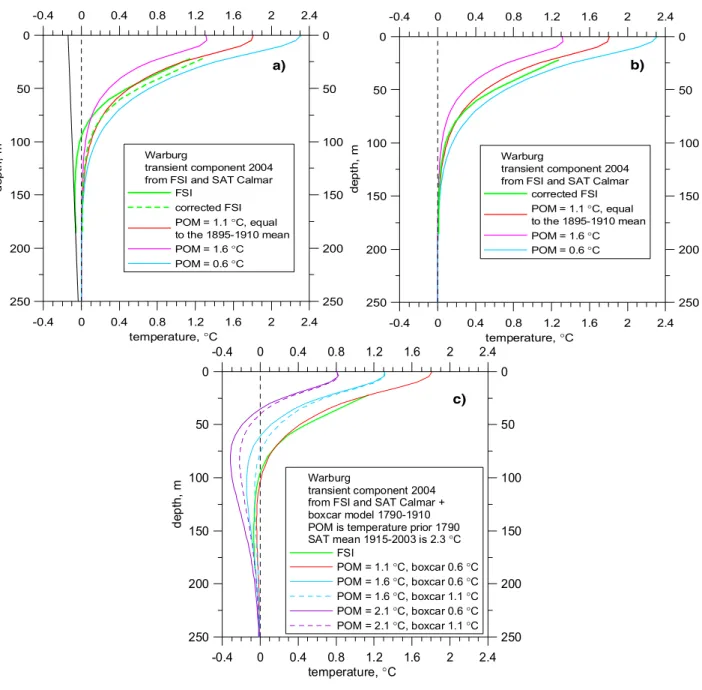
A comparison of the 2004 transient component of T-z in the borehole Warburg (Fig. 3) obtained as a posteriori FSI transients with the synthetic transients based on SAT series from Calmar (Fig. 4) which is representative of general SAT warming through the study area (Fig. 5) is shown in Fig. 6. The synthetic curves were calculated for several models:

1. POM equal to the 1895–1910 mean; 2. POM 0.5◦C higher than the above mean; 3. POM 0.5◦C lower than the mean; 4. SAT-boxcar low-POM

J. Majorowicz et al.: Paleoclimatic reconstructions in western Canada 5 -0.4 0 0.4 0.8 1.2 1.6 2 2.4 temperature, °C 250 200 150 100 50 0 d e p th , m 250 200 150 100 50 0 -0.4 0 0.4 0.8 1.2 1.6 2 2.4 Warburg transient component 2004 from FSI and SAT Calmar

FSI corrected FSI POM = 1.1 °C, equal to the 1895-1910 mean POM = 1.6 °C POM = 0.6 °C a) -0.4 0 0.4 0.8 1.2 1.6 2 2.4 temperature, °C 250 200 150 100 50 0 d e p th , m 250 200 150 100 50 0 -0.4 0 0.4 0.8 1.2 1.6 2 2.4 Warburg transient component 2004 from FSI and SAT Calmar

corrected FSI POM = 1.1 °C, equal to the 1895-1910 mean POM = 1.6 °C POM = 0.6 °C b) -0.4 0 0.4 0.8 1.2 1.6 2 2.4 temperature, °C 250 200 150 100 50 0 d ep th , m 250 200 150 100 50 0 -0.4 0 0.4 0.8 1.2 1.6 2 2.4 Warburg transient component 2004 from FSI and SAT Calmar + boxcar model 1790-1910 POM is temperature prior 1790 SAT mean 1915-2003 is 2.3 °C FSI POM = 1.1 °C, boxcar 0.6 °C POM = 1.6 °C, boxcar 0.6 °C POM = 1.6 °C, boxcar 1.1 °C POM = 2.1 °C, boxcar 0.6 °C POM = 2.1 °C, boxcar 1.1 °C c)

Fig. 6. Example of synthetic transient temperature-depth components for year 2004 AD based on Calmar surface temperature forcing and POM (pre-observational mean) assumed temperature. These are compared with FSI (functional space inversion) calculated transient for the 2004 log in well Warburg (Paskapoo Fm), (a) – upper left panel; “negative slope” corrected FSI calculated transient, (b) – upper right panel.

The best coincidence is exhibited by the model with POM=1.1◦C and the boxcar value 0.6◦C. It would suggest the long-term SAT mean

prior 1790 by about 0.5◦C lower than the SAT values shortly after the boxcar end in the period 1910–1930 (with the estimated mean 1.6◦C),

(c) – lower panel.

In model 4 the SAT data cover the period 1915–2003, their mean value is 2.3◦C. The mean of the first decade 1915– 1924 is 1.55◦C. The “boxcar” period is 1790–1910. The SAT value considered for the gap 1910–1915 is estimated in the same way as in previous calculations and amounts to 1.1◦C. There are two free parameters – a long-term mean prior 1790, which is referred to as POM, and the boxcar temperature between 1790 and 1910. The considered POM values are

centered ±0.5◦C around the mean of the first observational decade 1915–1924 and attain 1.1◦C, 1.6◦C and 2.1◦C. These values were combined with the boxcar temperatures 0.6◦C and 1.1◦C. In the case of POM=1.1◦C, only the boxcar value of 0.6◦C was considered. The results of modeling with use of a boxcar low event are shown in Fig. 6 (lower panel). The box-car – POM – SAT model described in the above point 4 we show in Fig. 7.

1750 1800 1850 1900 1950 2000 time, year -1 1 3 5 tem p er at ur e, ° C -1 1 3 5 1750 1800 1850 1900 1950 2000

Forcing surface temperature (POM before 1790, box-car event 1790 - 1910, the 1911-1914 estimate and the Calmar SAT 1915 -2004 series) < > > < POM range

box-car event range

Fig. 7. The surface temperature history used as a forcing function in simulating the subsurface temperature transient component shown in Fig. 6c. The lines’ colour and style before 1910 correspond to the transient curves shown in Fig. 6c.

Thermal diffusivity used in calculating the synthetic curves was the same as for the FSI, this means 0.7×10−6m2s−1in the case of Warburg.

We observe that the difference between synthetic and FSI curves is negative below circa 80 m in all cases (Fig. 5a). There could be several possible sources of the observed dis-agreement. One of them is a problem with short boreholes, where the FSI does not reproduce fully the recent warming. The FSI inversion scheme estimates the undisturbed basal heat flow, and therefore the transient component, by consid-ering a profile that extends to depths where recent climate changes have not affected the temperature profile (i.e. basal heat flow can be estimated accurately). In the case of shal-low boreholes it can result in a basal heat fshal-low estimate shal-lower than indicated by a gradient of the lowermost part of the log because of recent GST increases. One of the consequences underestimating basal heat flow would be a spurious mini-mum of the GST history, frequently observed in the recon-structions of wells shallower than 150 m (see simulations of the synthetic GST histories in Fig. 4 of Majorowicz et al., 2002) and an underestimate of warming amplitudes. We be-lieve that in the case of Warburg log modeled here, this is not the case due to its depth of 250 m, and other sources of the observed disagreement may be sought.

Tentatively, we tried to correct the above disagreement be-tween transients by fitting the lowermost part of a posteriori FSI transients in Fig. 6a to a line and by calculating new tran-sients as the difference of the old ones and the fitted lines. The resulting curve is shown by the dashed line and marked as “corrected FSI” (Fig. 6b). One can see that the degree of coincidence is appreciably better that in the case of the un-corrected one. The un-corrected FSI transients indicate that the

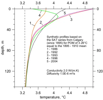
3.2 3.6 4 4.4 4.8 temperature, °C 120 80 40 0 de pt h, m 120 80 40 0 3.2 3.6 4 4.4 4.8

Synthetic profiles based on the SAT series from Calgary (since 1895) for POM of 3.26°C equal to the 1895 - 1910 mean 1 - 1986 2 - 1992 3 - 1993 4 - 1996 5 - 2004 Conductivity 2.0 W/(m.K) Diffusivity 1.0E-6 m2_/s 1 3 4 5 2

Fig. 8. Example of synthetic transient temperature-depth compo-nents for years 1992, 1993, 1996 and 2004 AD based on Calgary station surface temperature forcing and POM (pre-observational mean) assumed temperature level.

POM is 0 to −0.5◦C lower that the 1895–1910 means for the nearby Calmar SAT station.

Observed cooling at depth below ca. 100 m (Fig. 6a) may correspond to the cold period during the 1800s experienced in the prairies, but this is difficult to prove due to the lack of instrumental data before the 20th century. The transient component of the Warburg’s T-z log agrees with the GST low before recent warming showed in the upper ∼80 m of the T-z transient anomaly. Such temperature lows in the late 18th and all of the 19th century, preceding 20th century warm-ing, explains the negative slope of the T-z transient from measured logs well (Majorowicz et al., 1999, and this pa-per Fig. 6c). These lows are confirmed by recent tree ring reconstruction done in the Alberta Rocky Mountain (Luck-man et al., 1997; Luck(Luck-man and Wilson, 2005), at the western edge of the Western Canada Sedimentary basin.

One additional possible explanation of the disagreement between transient based on SAT-POM forcing models and measured transient below ca. 80 m is downward flow of groundwater. It will be discussed later in the paper.

Synthetic curves were also calculated for the Calgary SAT station for several years of the last decade (Fig. 8). A model of SAT-POM – equal to the 1895–1910 mean was used as forcing. The thermal diffusivity used in calcu-lating the synthetic curves was the same as for the FSI’s (i.e. 1.0×10−6m2s−1). We have used the thermal conductiv-ity model based on lithology description and literature (Jes-sop, 1990) assuming thermal conductivities and specific heat of 2 MJ/ (K m3).

J. Majorowicz et al.: Paleoclimatic reconstructions in western Canada 7

a)

b)

POM = 1910-1919 mean SAT

POM = -0.5 C (relative to 1910-1919 mean)

-0.5 0.0 0.5 1.0 1.5 2.0. 2.5 temperature, °C 300 200 100 0 d e p th , m 300 200 100 0 -0.5 0.0 0.5 1.0 1.5 2.0 2.5

Fig. 9. Comparison of transient temperature-depth components of temperature well logs analyzed by Majorowicz and Safanda (2001) for the Canadian Prairies (red curves) with synthetic transients (black curves; mean is marked by green curve) based on SAT-POM model for 22 SAT stations Banff, Calgary, Campsite, Fort Chipewyan, Fort Mc Murray, Gleichen, High Level, Lethbridge, Medicine Hat, Pincher Creek, R. M. House, Indian Head, Prince Albert, Regina, Saskatoon, Swift Current, Waseca, Birtle, Brandon, Dauphin, Morden and Winnipeg). POM level was assumed to be

equal to the 1910–1919 A.D. level (a) and POM=−0.5◦C (relative

to 1910–1919 mean).

The transients calculated independently of borehole mea-surements from the SAT-POM for all 22 SAT stations, (for locations see Fig. 5) when compared with transients calcu-lated from FSI’s of temperature logs in all 51 wells (loca-tions in Fig. 2) show significant difference below 70–80 m depth (Fig. 9) depending on the assumed POM illustrated in Fig. 10. Differences above the errors of measurement are in

1880 1900 1920 1940 1960 1980 2000 time, year -3 -2 -1 0 1 2 3 re d uc ed m e an a n nu al te m p er at ur e, oC -3 -2 -1 0 1 2 3 1880 1900 1920 1940 1960 1980 2000

Fig. 10. Surface temperatures from 22 Canadian stations and their POMs used as forcing functions in caclulating the synthetic tran-sients shown in Fig. 8a. Each curve was reduced by its 1961–1990

mean. The same curves, but with POMs shifted by −0.5◦C, were

used in calculating the transients shown in Fig. 8b.

the 70–200 m depth range. The simplification of the model used in the simulations is that POM is an assumed quantity.

The simulated T-z anomaly from SAT-POM model for Calgary (Fig. 8) can be compared with measurements of T-z in one location in Airdrie (Paskapoo Fm), Fig. 11. Deep regional geothermal gradient (25 mK/m) and regional steady state surface temperature 4◦C were used to extract the T-z anomaly. In this case it is apparent that T-z based on Cal-gary station SAT forcing is much higher than the observed T-z. Two explanations can be given: (1) SAT in Calgary is subject to an urban heat island effect; (2) changes in surface recharge and groundwater flow have disturbed the Airdrie T-z.

The above comparisons show that the observed changes in temperature-depth are only partly explained by the assumed SAT-POM forcing model.

5 Groundwater flow consideration

One of the well known possible causes of observed changes in the temperature-depth curve is vertical water flow (Brede-hoeft and Papadopulos, 1965; Reiter, 2005). Here, we an-alyze possible influence of such effect in the Paskapoo For-mation in the western part of Western Canada Sedimentary Basin.

5.1 Geological setting – Paskapoo Formation

The Paskapoo Formation is a mudstone dominated non-marine unit with a series of interbedded sand channels which can form isolated aquifer units. Channel sandstone beds range up to 15 m, but are typically 5–10 m thick. Sand

observed temperature anomalies climatic warming forcing anomaly

Depth (m) 0 0.2 0.4 0.6 0.8 1.0 0 20 60 80 40 Anomaly (°C)

Fig. 11. Comparison of T-z anomaly (transient) based on modelled SAT-POM for Calgary SAT station with one based on T-z logs in near by Airdrie well (Paskapoo Fm).

channels are lenticular and can pinch out laterally over short distances (100–150 m or more). However basal sand units can intercalate to form more extensive sheet sands. Sand units have a dominant intergranular porosity with a range from 5 to 30%, and averaging 19% over the formation. Sandstone permeability’s are typically very low (average 10−14_m2_{)with the exception of basal coarse-grained sand} units (∼10−12_m2_{). Limited paleocurrent data suggests a} general northeastward trend to channel sands suggesting that aquifer units within the Paskapoo have greater continuity on average along that orientation.

The fluvial sandstones of the Paskapoo are interbedded with light grey to greenish or brownish, sandy siltstone and. These fine grained facies form intervals several to several tens of metres thick between the major sandstone horizons and likely act as affective aquitards except where connected through fracture systems.

5.2 Modelling of groundwater flow and SAT forcing upon temperature – depth

The typical profile associated with downward flowing groundwater creates a lower downward curvature (Brede-hoeft and Papadopulos, 1965, and Reiter, 2005). This tends to show up as recent warming in the upper part of the profile and cooling at depth when ’corrected’ from a linear geother-mal gradient, assuming that the temperature profile can be described by Eq. (2). This equation neglects advective heat flow. The type of perturbation that would be associated with downward flow of groundwater depends on recharge rates, depth and time.

Stallman (1963) provided differential equation that de-scribes the flow of heat and ground water in one dimension for a homogeneous and isotropic porous medium:

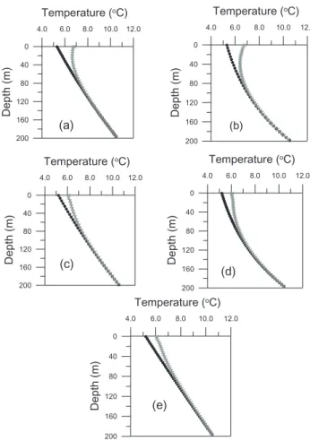
κe ∂2T ∂z2 −cfρf ∂ (vzT ) ∂z =csatρsat ∂T ∂t (5) 4.0 6.0 8.0 10.0 12.0 Temperature (o_C) 200 160 120 80 40 0 D epth (m) (d) 4.0 6.0 8.0 10.0 12.0 Temperature (o_C) 200 160 120 80 40 0 De pth (m) (c) 4.0 6.0 8.0 10.0 12.0 Temperature (o_C) 200 160 120 80 40 0 D epth (m) (a) 4.0 6.0 8.0 10.0 12.0 Temperature (o_C) 200 160 120 80 40 0 De pth (m) (b) 4.0 6.0 8.0 10.0 12.0 Temperature (o_C) 200 160 120 80 40 0 De pth (m) (e)

Fig. 12. Comparison of T-z logs calculated using SAT forcing based on Calmar (a, b) and Calgary (c, d) stations and assumed ground water recharge rates of 25 mm/year (a, c) and 100 mm/ year (b, d). The model results with a 5 mm/yr model for the Calgary SAT (e) show the temperature profile is pretty straight for a recharge rate this low.

where keis thermal effective conductivity, T is temperature,

cf is the specific heat of water, ρf is the density of water, vz is specific discharge, csatis the specific heat capacity of the saturated porous medium and ρsatis the density of the satu-rated porous medium. This assumes steady-state fluid flow, which likely is not the case. However, it appears that dras-tic hydrological changes would have to occur before this be-comes an important issue. In the current study, this equation is solved numerically using MULTIFLO (Painter and Seth, 2003), which utilizes an integrated finite difference formula-tion

The results of the advective-conductive models assuming groundwater recharge rates of 25 and 100 mm/yr were calcu-lated in this paper for Calgary and Calmar stations assuming SAT records as forcing (Fig. 12). The method described in detail by Ferguson and Woodbury (2005) was used. We have estimated the approximate surface temperature to which the SAT anomalies are added or subtracted from by extrapolat-ing the Airdrie and Calmar profiles to the surface, (5.2 and

J. Majorowicz et al.: Paleoclimatic reconstructions in western Canada 9 5.3◦_{C, respectively). We have used a fixed temperature at}

the bottom of the aquifer and fixed pressure boundary con-dition. In both cases we have used a temperature of 10.6◦_C at the base of the model at 200 m, based on an extrapolation of the Warburg log. These models are by no means perfect because we know little about the seepage velocities of water over the broader area, and there is most likely horizontal flow of groundwater that should be considered as well. Recent es-timates for long term recharge rates into the Paskapoo For-mation in the Spyhill area north of Calgary suggest minimal recharge rates (∼5 mm/yr, T. Van Dijk, personal communi-cation, 2005). For this very low value, 5 mm/year, model T-z shows no curvature.

While the high end recharge rate used here suggests that for the extreme case some of the observed curvature in the profiles, especially the Warburg profile, could be due to groundwater flow, it is more likely that the low recharge rates in this semi-arid region would have minimal impact.

6 Discussion and conclusions

Modelling and observations presented above show that dif-ferences higher than the error of measurement are observed between the model based on surface forcing (observed SAT plus assumed POM) and observation. It is mainly due to our poor knowledge of the climatic history before the ob-servational period and poor knowledge of other factors like groundwater flow, snow cover trends etc. These factors are difficult to distinguish from each other without additional in-dependent information about the climate preceding the ob-servational SAT record.

The transients shown here for all of Alberta and S. Saskatchewan (51 wells) and transients modeled here for 22 SAT stations (Fig. 9) agree well with the example an-alyzed for the Paskapoo Fm well in Warburg (Fig. 6) de-spite the fact that the majority of wells are outside the area of Paskapoo. There are only 11 Paskapoo logs available (Fig. 3). Significant disagreement exists between modelled transients of T-z SAT-POM models and transients based on measured T-z profiles. The disagreement is most significant in the 70–200 m depth interval.

A “Box-car” model approximating lower temperature in 1800’s preceding 20th century warming used by Majorow-icz et al. (1999) and this paper (Figs. 6c, 7) can explain the observed discrepancy and model the observed negative slope of temperature transients below 80 m depth. While the ob-served cooling at this depth may correspond to the cold pe-riod during the 1800’s experienced in the prairies, it is diffi-cult to prove due to the lack of instrumental data. There is support of the above explanations in proxy record from tree rings in the Alberta Rocky Mountain’s Colombia glacier re-gion (Luckman et al., 1997; Luckman and Wilson, 2005). A temperature low of the late 1700s through 1800’s is apparent from the tree ring based temperature history reconstruction

of Luckman et al. (1997). These data however, unlike well temperature based reconstructions are based on growing sea-son only and do not contain the same information.

Groundwater flow was examined as another possible ex-planation. Downward groundwater flow creates T-z curva-ture and this tends to show up as recent warming in the upper part of the profile and cooling at depth when reduced. How-ever, proxy SAT reconstructions indicate that 1800s cooling was present and this would be enough to explain T-z obser-vations. If this is the case, it would be consistent with recent work suggesting long term recharge rates are significantly lower than the modeled 100 mm/year. Even models using recharge rates (25 mm/yr) at five times the estimated average values do provide evidence that groundwater flow could sig-nificantly affect temperature profile. Thus the temperature-depth curve in this region can be explained to a large extend by surface cooling/warming models alone, without assump-tion of significant advective heat transport.

While most of the observed transients can be explained by surface temperature change, the deviation of the sients from well temperature logs from the synthetic tran-sients based on SAT-POM model exists. Assuming lower POM’s will make that difference even larger. However, the assumed POM constant level of temperature before the start of observations in the early 20th century may not be valid and the local 19th century surface temperature low related to Little Ice Age could explain observed temperature’s transient (Majorowicz et al., 1999).

The results show that in the data set presented here, SAT forcing is the main driving factor for the underground tem-perature changes diffusing with depth. It supports validity of borehole temperature paleoclimatology hypothesis that the ground surface temperature is systematically coupled with the air temperature over time periods of decades). The anal-ysis of the transient temperatures with depth presented here also supports the validity of the assumption that the changes in ground surface temperature diffuses mainly by conduction into the subsurface and impose a transient “climate” signal on the steady-state geothermal gradient. These are limited to the sites in which no hydrogeological disturbance or land surface changes were observed.

Acknowledgements. We would like to thank Environment Alberta and Saskatoon Research Council for giving us access to the well sites. Ed. J. Jaworski (S.R.C) and Metro Magas (Environment Al-berta emeritus) assisted with guidance and removal of the piezome-ters for the time of logging of temperature.

Comments of anonymous referee and V. Rath were very helpful in constructing a final version of this paper.

This material is partially based upon work supported by the GSC Calgary , EC Downsview and the NSF under Grant No. 0318384. Edited by: V. Rath

References

Baker, D. G. and Ruschy, D. L.: The recent warming in eastern Minnesota shown by ground temperatures, Geophys. Res. Lett., 20, 371–374, 1993.

Beach, R. D. W., Jones, F. W., and Majorowicz, J. A.: Heat flow and heat generation for the Churchill of Western Canadian Sedi-mentary basin, Geothermics, 16, 1–16, 1987.

Bredehoeft, J. D. and Papadopulos, I. S.: Rates of vertical ground-water movement estimated from the Earth’s thermal profile, Wa-ter Resour. Res., 1, 325–328, 1965.

Beltrami, H.: On the relationship between ground temperature his-tories and meteorological records: a report on the Pomquet sta-tion, Global Planet. Change, 29, 327–348, 2001.

Cermak, V.: Underground temperature and inferred climatic tem-perature of the past millennium, Paleography, Paleoecclimatol-ogy, PaleoecolPaleoecclimatol-ogy, 10, 1–19, 1971.

Cermak, V., Bodri, L., Gosnold, W. D., and Jessop, A. M.: Most recent climate history stored in the sub-surface, inversion of tem-perature logs re-measured after 30 years, Geophys. Res. Abstr., 5, 02117 EGS-AGU-UEG Nice, France, 2003.

Carslaw, H. S. and Jaeger, J. C.: Conduction of Heat in Solids Ox-ford Univ. Press, New York, 386 pp., 1959.

Environment Canada: The state of Canada’s climate: Monitoring variability and change, SOE A State of Environment Report, 95, 52 p., 1995.

Ferguson, G. and Woodbury, A. D.: The Effect of Climatic Vari-ability on Estimates of Recharge derived from Temperature Data, Ground Water, 43(6), 937–842, 2005.

Gonzalez-Rouco, F., von Stroch, H., and Zorita, E.: Deep soil tem-perature as proxy for surface air-temtem-perature in a coupled model simulation of the last thousand years, Geophys. Res. Lett., 30, 21, doi:10.1029/2003GL018264, 2003.

Gosnold, W. D., Todhunter, P. E., and Schmidt, W.: The borehole temperature record of climate warming in the mid-continent of north America, Global and Planetary Change, 15, 33–45, 1997. Huang, S., Pollack, H. N., and Shen, P.-Y.: Temperature trends over

the past five centuries reconstructed from borehole temperatures, Nature, 403, 756–758, 2000.

Jessop, A. M.: Thermal Geophysics, Developments in Solid Earth, Geophysics, 17, Elsevier, 306 p., 1990.

Jones, P. D. and Mann, M. E.: Climate over past millennia, Rev. Geophys., 42, 1–42, Elsevier, 2004.

Kane, D. L., Hinkel, K. M., Goering, D. J., Hinzman, L. D., and Outcalt, S. I.: Non-conductive heat transfer associated with frozen soils, Global Planet.Change, 29, 275–292, 2001. Lewis, T. and Skinner, W.: Inferring climate change from

under-ground temperatures: Apparent climatic stability and apparent climatic warming, Earth Interactions, 7, paper No. 9, 1–9, 2003. Lachenbruch, A. H.: Permafrost, the active layer and changing cli-mate, U.S. Geol. Surv., open-file report, 94–694, Menlo Park, CA, 1994, 43 pp., 1994.

Luckman, B. H. and Wilson, R. J. S.: Summer temperatures in the canadian rockies during the last millennium: a revised record, Climate Dynamics, 24, 131–144, 2005.

Luckman, B. H., Briffa, K. R., Jones, P. D., and Schwaingruber, F. H.: Tree ring based reconstruction of summer temperatures at the Columbia Icefield, Alberta, Canada, AD 1073–1983, The Holocene, 7, 375–389, 1997.

Majorowicz, J. A. and Skinner, W. R.: Potential causes of dif-ferences between ground and surface air temperature warming across different ecozones in Alberta, Canada, Global and Plane-tary Change, 15, 79–91, 1997.

Majorowicz, J. A. and Safanda, J.: Composite surface temperature history from simultaneous inversion of borehole temperatures in Western Canadian plains, Global Planet. Change, 29, 231–239, 2001.

Majorowicz, J. A., Safanda, J., Harris, R., and Skinner, W. R.: Large ground surface temperature changes of the last three cen-turies inferred from borehole temperatures in the southern Cana-dian prairies-Saskatchewan, Global Planet. Change, 20, 227– 241, 1999.

Majorowicz, J. A., Safanda, J., and Skinner, W.: East to west retar-dation in the onset of the recent warming across Canada inferred from inversions of temperature logs, J. Geophys. Res., 107(B10), 2227–2002, 2002.

Mann, M. E. and Schmidt, G. A.: Ground vs. Surface Air

Temperature Trends: Implications for Borehole Surface Tem-perature Reconstructions, Geophys. Res. Lett., 30(12), 1607, doi:10.1029/2003GL017170 2003.

Painter, S. and Seth, M. S.: MULTIFLO User’s Manual; MULTI-FLO Version 2.0., Southwest Research Institute, San Antonio, Texas, 2003.

Putnam, S. N. and Chapman, D. S.: A geothermal climate change observatory: first year results from Emigrant Pass in Northwest Utah, J. Geophys. Res., 101, 21 877–21 890, 1996.

Pollack, H. N., Shauopeng, H., and Shen, P.-Y.: Climate change record in subsurface temperatures: a global perspective, Science, 282, 279–281, 2000.

Reiter, M.: Possible ambiguities in subsurface temperature logs: consideration of ground-water flow and ground surface tempera-ture change, Pure and Applied Geophys., 162, 343–355, 2005. Shen, P.-Y. and Beck, A. E.: Least squares inversion of borehole

temperature measurements in functional space, J. Geophys. Res, 96, 19 965–19 979, 1991.

Schmidt, W. L. Gosnold, W. D., and Enz, J. W.: A decade of air-ground temperature exchange from Fargo North Dakota, Global Planet. Change, 29, 311–325, 2001.

Skinner, W. R. and Majorowicz, J. A.: Regional climatic warming and associated twentieth century land-cover changes in north-western North America, Climate Research, 12, 39–52, 1999. Stallman, R. W.: Computation of ground-water velocity from

tem-perature data, in: Method of Collecting and Interpreting Ground-Water Data, edited by: Bentall, R., Ground-Water Supply Paper 1544-H, Washington, D.C., USGS, 36–46, 1963.

Stieglitz, M., Romanovsky, V. E., and Osterkamp, T. E.: The role of snow cover in the warming of arctic permafrost, Geophys. Res. Lett., 30, 1721, doi:10,1029/2003GL017337, 2003.

Vincent, L.: A technique for the identification of inhomogeneities in Canadian temperature series, J. Climate, 11, 1094–1104, 1998. Vincent, L. and Gullett, D. W.: Canadian historical and

homoge-neous temperature datasets for climate change analyses, Int. J. Clim., 19, 1375–1388, 1999.

Zhang, X., Vincent, L. A., Hogg, D. W., and Niitsoo, A.: Temper-ature and precipitation trends in Canada during the 20th century, Atmosphere-Ocean, 38, 395–429, 2000.