Do firms want to borrow more? : testing credit constraints using a directed lending program

Digitized

by

the

Internet

Archive

in

2011

with

funding

from

Boston

Library

Consortium

Member

Libraries

HB31

.M415

dewsy

Massachusetts

Institute

of

Technology

Department

of

Economics

Working

Paper

Series

DO

FIRMS

WANT

TO

BORROW

MORE?

TESTING CREDIT

CONSTRAINTS USING

A

DIRECTED

LENDING

PROGRAM*

Abhijit

Banerjee

Esther

Duflo

Working

Paper

02-25

May

2002

Room

E52-251

50

Memorial

Drive

Cambridge,

MA

02142

This

paper

can be downloaded

without

charge from

the

Social

Science

Research Network Paper

Collection

at

http://papers. ssrn,com/paper.taf?abstract id=316587

MASSACHOSEtlTiwSTFfirTr

^FTECHNOLOGY

AUG

_{1 2}

2002

Massachusetts

Institute

of

Technology

Department

of

Economics

Working

Paper

Series

DO

FIRMS

WANT

TO

BORROW

MORE?

TESTING

CREDIT

CONSTRAINTS USING

A

DIRECTED

LENDING

PROGRAM*

Abhijit

Banerjee

Esther

Duflo

Working

Paper

02-25

May

2002

Room

E52-251

50

Memorial

Drive

Cambridge,

MA

02142

This

paper can be

downloaded

without

charge

from

the

Social

Science

Research Network Paper

Collection

at

Do

Firms

Want

to

Borrow

More?

Testing Credit Constraints

Using a

Directed

Lending

Program

1

*

Abhijit

V.

BanerjeeWd

Esther

Duflo*

May

2002

Abstract

We

begin the paper by laying out a simple methodology that allows us to determine

whether firms are credit constrained, based on

how

they react to changes in directed

lend-ing programs.

The

basic idea is that while both constrained and unconstrained firms

may

be willing to absorb all the directed credit that they can get (because it

may

be cheaper

than other sources of credit), constrained firmswill use it to expand production, while un-constrained firms will primarily use it as a substitute for other borrowing.

We

the apply

this methodology to firms in India that

became

eligible for directed credit as a result of a

policy changein 1998. Using firmsthat werealready getting this kindofcreditbefore 1998

to control for time trends,

we

show that there is no evidence that directed credit is being

used as a substitute for other forms ofcredit. Instead the credit was used to financemore

production-there was significant acceleration in the rate ofgrowth of sales and profits for

thesefirms.

We

conclude that

many

ofthe firmsmust havebeenseverely creditconstrained.

Keywords: Banking, Credit constraints, India JEL: 016,

G2

*We

thank Tata Consulting Services for their help in understanding the Indian banking Industry,

Sankarnaranayan for his work collecting the data, Dean Yang and Niki Klonaris for excellent research

assis-tance, and Robert Barro, Sugato Battacharya, Gary Becker, Ehanan Helpman, Sendhil Mullainathan, Kevin

Murphy, Raghuram Rajan and Christopher Udryfor veryuseful comments.

We

are particularly grateful to the

administrationandthe employeesofthebankwestudyfortheirgiving us access tothedataweuseinthispaper,

department ofEconomics, MIT.

1

Introduction

That

there are limits to access to credit is widely accepted today as

an

important part of

an

economist's description of the world. Credit constraints

now

figure prominently in

economic

analyzes ofshort-termfluctuations

and

long-term growth.1

Yet

one

is hard-pressed tofind tight

evidenceofthe existence ofcreditconstraints

on

firms, especiallyina developing countrysetting.

This is in

some

ways

what

is to

be

expected: a firm is credit constrained

when

it cannot

borrow

as

much

asit

would

liketoatthegoing

market

rateor, inotherwords,

when

themarginal

productofcapital inthe firmisgreater

than

the

market

interest rate. It is

however

notclear

how

one should go about estimating the marginal product ofcapital.

The

most

obvious approach,

which

relies

on

usingshockstothe

market

supply curveofcapitaltoestimatethe

demand

curve,

is onlyvalid under the

assumption

that thesupply is always equal to

demand,

i.e., ifthe firm is

never credit constrained.

The

literature has therefore taken a less direct route:

The

idea is to study the effects of

access to

what

are taken to

be

close substitutes for credit

—

current cash flow, parental wealth,

community

wealth

—

on

investment. Ifthere are

no

credit constraints, greater access to a

substi-tutefor credit

would

beirrelevant for theinvestment decision.

While

thisliteraturehastypically

found

that thesecredit substitutes

do

affect investment,2 suggesting that firms areindeed credit

constrained, the interpretation of this evidence is not uncontroversial.

The

problem

is that

ac-cess to these other resources is unlikely to be entirely uncorrelated with other characteristics

ofthe firm (such as productivity) that

may

influence

how much

it

wants

to invest.

To

take

an

obvious example, a shock to cash-flow potentially contains information about the firm's future

performance.

Of

course, ifone has

enough

information

about

the shock, one can isolate shocks

that are clearly uninformative.

Lamont's

(1997) use of oil-price shocks to look at non-oil

in-vestment of oil

companies

is

an example

ofthis strategy.

However

it is not an accident that

'SeeBernanke andGertler (1989)andKiyotakiandMoore(1997)ontheories of business cyclesbased oncredit

constraints,andBanerjeeand

Newman

(1993) andGalorandZeira (1993)ontheoriesofgrowthanddevelopment based on limitedcredit access.

Theliterature onthe effectsofcash-flowon investment isenormous. Fazzari, Hubbard and Petersen (1998) provide ausefulintroduction to this literature. Theeffectsof familywealthoninvestment have alsobeen

exten-sivelystudied (seeBlanchflowerandOswald (1998),foraninterestingexample). Thereisalsoa growingliterature

the

companies

for

which

Lamont

is able to have precise

enough

information about thenature of

shocks tend to be very large

companies

and, as

emphasized by

Lamont

and

others, 3 cash-flow

shocks canhave very different effects

on

big cash-rich firms

than

on

small cash-poorfirms.4

Here

we

take a different

approach

to this question.

We

make

use of a policy change that

affected the flow of directed credit to

an

identifiable subset of firms.

Such

policy changes are

common

in

many

developing

and

developed countries

—

even the U.S. has the

Community

Rein-vestment Act,

which

obliges

banks

to lend

more

to specific communities.5

The

advantageofour

approach

isthat it givesus aspecific exogenous shocktothesupply of

credit to specific firms (as

compared

to a shift in the overallsupply ofcredit). Its disadvantage

isthat directed credit need not

be

priced at its true

market

price,

and

therefore a shock to the

supply ofdirected credit mightlead to

more

investmentevenifthe firmisnotcredit constrained.

In this paper

we

develop a simple

methodology

based

on

ideas

from

elementaryprice theory

that allows to deal with this problem.

The

methodology

is based

on two

observations: first, if

a firm is not credit constrained then an increase in the supply ofsubsidized directed credit to

the firm

must

lead it to substitute directed credit for credit

from

the market. Second, while

investment

and

thereforetotal production

may

go

up

even ifthe firm is not credit constrained,

itwill onlygo

up

ifthe firm has already fully substituted

market

credit with directed credit.

We

test these implications using firm-level datathat

we

collected

from

a

sample

of small to

medium

size firmsin India.

We

make

use of achange in theso-called priority sector regulation,

under

which

firms smaller than a certain limit are given priority access to

bank

lending.6

The

experiment

we

exploit is a 1998 reform

which

increased the

maximum

size below

which

a firm

is eligible to receive priority sector lending.

Our

basic empirical strategy is a difference-in-difference-in-difference approach: that is,

we

focus

on

the changes in the rate of change in

3

Kaplan and Zingales (2000) make thesamepoint.

4

The estimation of the effects of credit constraints on farmers is significantly more straightforward since variations in theweather providea powerfulsource ofexogeneous short-term variation in cashflow. Rosenzweig

and Wolpin (1993) use this strategy to study theeffect ofcredit constraints on investment in bullocks in rural

India.

5_Zinman

(2002) evaluates theeffect ofcredit on small businesses using exogenous variations induced by the

CommunityReinvestmentAct.

6

Banks arepenalized for failingtolend acertain fraction ofthe portfolio to firms that classifiedto bein the

various firm

outcomes

before

and

after the reform for firms that got included in the priority

sector as aresult ofthe

new

limit, using the corresponding changes for firms that were already

in theprioritysector as acontrol.

We

find that

bank

lending

and

firmrevenues

went

up

for the

newly

targeted firmsinthe year of the reform.

We

find

no

evidencethatthis

was accompanied by

substitution of

bank

credit for borrowing

from

the

market

and no

evidencethat revenue

growth

was

confined to firms that

had

fully substituted

bank

credit for

market

borrowing.

As

already

argued, the last

two

observations are inconsistent with the firms being unconstrained in their

market

borrowing.

We

alsousethis datatoestimate parametersoftheproductionfunction.

We

find

no

evidence ofdiminishing returns to additional investment,

which

reinforces the idea that

the firms arenotatthe point

where

themarginalproduct is

about

tofall

below

theinterest rate.

Finally,

we

try to estimate the effect ofthe

program-induced

additional investment

on

profits.

While

the interpretation ofthis result relies

on

some

additional assumptions, it suggests a very

large

gap between

the marginalproduct

and

the

market

interest rate (the point estimateisthat

Rs. 1

more

in loans increased profits net ofinterest

payment by

Rs. 1.36,

which

is

much

too

large to

be

explained as just the effect ofgetting a subsidized loan).

The

rest of the paper is organized as follows: the next section describes the institutional

environment

and

our

data

sources, provides

some

descriptive evidence

and

informally argues

that firms

may

be

expected to

be

credit constrained in this environment.

The

next section

develops our empirical strategy, starting with the theory

and

ending with the equation

we

estimate.

The

penultimate section reports the results.

We

conclude with

some

admittedly

speculative discussion of

what

our results imply forcredit policy in India.

2

Institutions,

Data and

Some

Descriptive

Evidence

2.1

The

Banking

Sector

in

India

Despitethe

emergence

ofa

number

of

dynamic

private sector

banks

and

entry

by

a large

number

offoreignbanks, the biggest

banks

inIndia areallin the publicsector, i.e., they are corporatized

banks

with the

government

as the controlling share-holder.

The

27 public sector

banks

collect

over

77%

ofdeposits

and

comprise over

90%

ofall branches.

requirements not to revealthe

name

ofthebank,

we

note it

was

rated

among

the topfive public

sector banks in 1999

and

2000

by

Business Today, a

major

business magazine.

While banks

inIndia occasionally providelonger-termloans,financingfixedcapitalis

primar-ilytheresponsibility of specializedlong-term lendinginstitutions such asthe IndustrialFinance

Corporation ofIndia.

Banks

typically provide short-term working capitaltofirms.

These

loans

are given as acredit linewith apre-specified limit

and an

interestratethat issetafew

percent-agepoints aboveprime.

The

gap

betweenthe interestrate

and

theprimerateisfixed in advance

based on the firm's creditrating

and

other characteristics, butcannot be

more

than

4%.

Credit

lines in India charge interest only

on

the part that is used and, given that the interest rate is pre-specified,

many

borrowers

want

as large acredit line as theycan get.

2.2

Priority

Sector

Regulation

All

banks

are required to lend at least

40%

of their net credit to the "priority sector",

which

includes agriculture, agricultural processing, transport industry,

and

smallscaleindustry (SSI).

If banks

do

not satisfy the priority sector target, they are required to lend

money

to specific

government

agenciesat very low rates of interest.

In

January

1998, there

was

a change in the definition of the small scale industry sector.

Before thisdate only firms with total investment inplant

and

machinery below Rs. 6.5 million

were included in the priority sector.

The

reform extended the definition of priority sector to

include firms with investment in plants

and machinery

up

to Rs. 30 million.

The

"priority sector" targets

seem

to be binding for the

bank

we

study (as well as for

most

banks): every year, the bank's sharelent tothe priority sector isvery closeto

40%

(it

was

42%

in 2000-2001). It is plausible that the

bank had

to go

some

distance

down

the client quality

ladder to achieve this target. Moreover, there is the issue ofthe physical cost of lending. In a

previousstudy ofthis

and

threeother

banks

(Banerjee

and

Duflo, 2000),

we

calculated that the

labor

and

administrative costs associated to lending to the SSI sector

was

about 1.5 paisa per

Rupee

higher than that oflendingin theunreserved sector. This isconsistent with the

common

view that lending to smaller clients is

more

costly.

Two

things

changed

when

the priority sector limit

was

raised: first, the

bank

could

draw

from

a larger pool

and

therefore could be

more

exactingin its standards for clients. Second, it

could save

on

the cost oflending

by

focusing

on

slightly larger clients. For

both

these reasons the

bank would

like to switch its lending towards the

newly

inducted

members

ofthe priority sector. Ifthese firms were constrained in their

demand

for credit before the policychange, one

would

expect tosee

an

expansion of lendingto these firms relative to firms that were already in

the priority sector.7

2.3

Data

Collection

The

data for this study were obtained

from one

ofthe better-performing Indian public sector

banks. This bank, like other public sectorbanks, routinely collects balancesheet

and

profit

and

loss account data

from

all firms that

borrow from

it

and

compiles the data in the firm's loan

folder.

Every

year the firm also

must

apply for renewal/extension of its credit line,

and

the

paper-work for this is also stored in the folder, along with the firm's initial application.

The

folderis typically stored in the

branch

until it is completely full.

With

the help of employees

from

this bank, as well as a former

bank

officer,

we

extracted

data

from

the loan folders in the spring of 2000.

We

collected general information about the

client (product description, investment in plant

and

machinery, date of incorporation ofunits,

length orthe relationshipwiththebank, currentlimits for

term

loans,

working

capital,

and

letter

ofcredit).

We

also recorded a

summary

ofthe balance sheet

and

profit

and

loss information

collected

by

thebank, as well as information

about

thebank's decisionregarding the

amount

of

credit to extend tothe firm,

and

the interest rate charged.

As

we

discuss in

more

detail below, part ofour empirical strategy called for a

comparison

between

accounts that have always

been

a part of thepriority sector,

and

accountsthat

became

part of the priority sector in 1998.

We

first selected all the branches that handle business

accounts in the 6

major

regions of the bank's operation (including

New

Delhi

and Mumbai).

In

each ofthese branches,

we

collected information

on

all the accounts belonging to the priority

sector.

We

collected data

on

atotal of 253 firms, including 93 firms with investment in plants Theincrease in lending to larger firms

may

come entirely atthe expenseofsmaller firms (without affecting

total lending to the priority sector), or the reform could cause an increase in the amount lent to the priority sector.

We

will focus on the comparison between firms that were newly labelled aspriority sector and smaller

and machinery between

6.5

and

30 million rupees.

We

aimed

tocollect datafor the years

1996-1999, but

when

a folder is full, older information is not always kept in the branch.

We

have

1996data

on

lending for 120 accounts (ofthe 166 firmsthat

had

started their relationshipwith

the

banks by

1996), 1997 data for 175 accounts (of 191 possible accounts), 1998 data for 226

accounts (of 238),

and

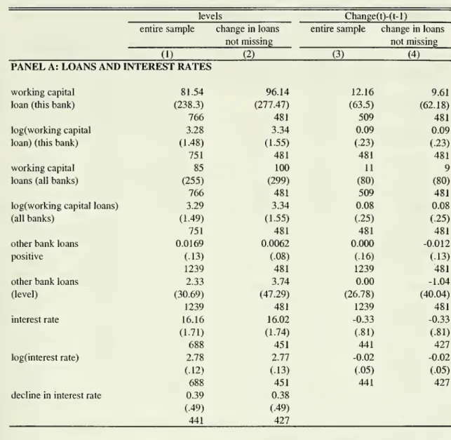
1999 data for 240 accounts. Table 1 presents the

summary

statistics for

all data that will be used in the analysis of credit constraint

and

credit rationing (in the full

sample,

and

in the sample for

which

we

have information

on

the change in lending

between

the

previous period

and

that period,

which

will be the

sample

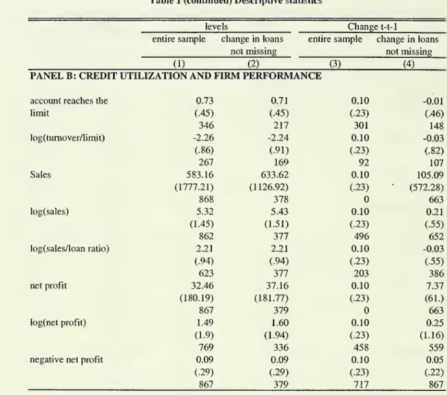
ofinterest for the analysis).

2.4

Descriptive

Evidence

on Lending

Decisions

Inthissubsection,

we

provide

some

description oflending decisionsinthe

banking

sector.

We

use

thisevidence to argue that this is

an

environment

where

credit constraints arisequite naturally.

Tables 2

and

3

show

descriptive statistics regarding the loans in the sample.

The

first

row

oftable 2

shows

that, in a majority ofcases, the loan limit does not change

from

year to year:

in 1999, the limit

was

not

updated

even in

nominal

terms for

65%

of the loans. This is not

because thelimit is set so high that it is essentially non-binding:

row

2

shows

that in the three

years in the sample,

69%

to

80%

ofthe accounts reached or exceeded the credit limit at least

once in theyear.

Thislack of

growth

in thecredit limit granted

by

the

bank

isparticularly striking giventhat

theIndian

economy

registered

nominal

growth

rates of over

12%

per year. This

would

suggest

that the

demand

for

bank

credit should haveincreased

from

year to year over the period, unless

the firms have increasing access to another source of finance.

There

is

no

evidence that they

wereusing

any

other formalsource ofcredit for

working

capital.

On

average

98%

oftheworking

capitalloans providedto firms inour

sample

come

from

this one

bank and

in

any

case, the

same

kind ofinertia

shows

up

in the data

on

total

bank

loans to. the firm.

That

the

demand

forformalsectorcredit increased

from

year toyear, issuggested

by

rows4

and

5 in table 2.

The

bank'sofficial guidelines for lending explicitlystate that the

bank

should

try to

meet

the legitimate needs ofthe borrower. For this reason, the

maximum

lending limits

that can be authorized

by

the

bank

are explicitly linked to the projected sales of the borrower.

lendinglimit

on

the basis of the turnover.8

Row

3

shows

that actual sales have increased

from

year to year for

most

firms.

Rows

4

and

5

show

that

both

projected sales

and

the

maximum

authorizedlendingalsoincreased

from

year to yearin a largemajorityofcases. Yet there

was no

correspondingchange inlending

from

thebank.

The

changein the credit limitthat

was

actually

sanctioned thus fell systematically short of

what

the

bank

determined to be the firm's needs

as determined

by

the bank. In 1999,

80%

of the actual limits granted were below

20%

ofthe

predicted sales,

and

60%

were

below

the

maximum

limit calculated

by

the banker.

On

average,

thegranted limit

was

89%

ofthe

maximum

authorizedlimit,

and

67%

of

what

followingtherule

based

on

20%

ofpredicted sales

would

give. Itis possible that

some

oftheshortfall

was

covered

by

informalcredit, includingtradecredit: accordingto thebalancesheet, totalcurrentliabilities

excluding

bank

credit increased

by

3.8%

every year

on

average.9

However,

some

expenses (such

aswages) aretypically not covered

by

tradecredit and, moreover, trade credit could berationed

as well.

The

question that is at the heart of this paper is

whether

suchsubstitution operates to

the point

where

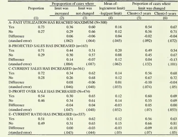
a firm isnot credit constrained.

In table 3,

we

examine

in

more

detail

whether

this tendency could

be

explained

by

other

factors that

might

have affected a firm's need for credit.

Column

(3)

shows

that

no

variable

we

observe

seems

to explain

why

afirm's credit limit

was

changed: firms arenot

more

likely to get

an

increase in limit ifthey reached the

maximum

limit in the previous year, iftheir projected

sales (according to the bank itself)

have

increased, if their current sales have increased, if the

ratio ofprofitstosaleshas increased, orifthe currentratio (the ratioofcurrentassetstocurrent

liabilities, a traditional indicator of

how

secure a

working

capital loan is, in India as well as in

the U.S.) has increased.

Turning

to thedirection or the

magnitude

ofchanges, only

an

increase

in projected sales or current sales predicts

an

increase in granted limit,

and

only an increase in

projected salespredict thelevelofincrease. This couldwell be

due

to reversecausality, however:

The

bank

officer could

be

more

likely to predict a larger increase in sales

when

he is willing to give a larger credit extension to the firm.

One

reasonthegranted limit

may

not change isthat the previous year's limit already

incor-8

Theexact ruleisthat the limitonturnover basis shouldbe the

minimum

of20% ofthe projectedsales and 25% oftheprojectedsalesminusthe finances available to the firmfrom other sources. In practice, the

maximum

limitcalculated by thebank officeris not alwaysequal to thiscalculated number.

porated all information relevant to the lending decision: the limit is not responsive to

what

is

currently going

on

in the firm, because these are just short-run fluctuations

which

tell us little

about the future of the firm. Ifthis were the case,

we

should observe that granted limits are

much

more

responsive to these factors for

young

firms than for old firms.

Columns

5

and

6 in

table 3 repeat the analysis, breaking the

sample

into recent

and

older clients.

Changes

in limits

are

more

frequent foryounger clients, but they

do

not

seem

to

be

more

sensitive toeither past

utilization, increases in projected sales, or profits.

The

fact that the probability of a limit's change is entirely

uncorrected

with observable

firm characteristics is striking.

One

plausible theory relates this to the fact, noted above, that

changes in the limit are surprisingly rare. If

bank

officials are reluctant to change the limit,

a large fraction of the observed changes

may

reflect effective lobbying or something purely

procedural ("it has been fiveyears since the limit

was

raised") ratherthan

economic

rationality.

What

explains the reluctance of loan officers to

do

what

is, palpably, their job?

A

recent

report

on

banking policies

commissioned by

the Reserve

Bank

of India suggests one potential

explanation:

"The

[working group] observed that it has received representations

from

the

man-agement and

the unions ofthe

bank

complaining about the diffidence in taking credit decisions with

which

the

banks

are beset at present. This is

due

to investigations

by

outside agencies

on

the accountability ofstaffin respect to

Non

Performing Assets."

(Tannan

(2001)). In other

words, the

problem

is that changing the limit (in either direction) involves sticking one's neck

out-ifone cuts the limit the firm

may

complain,

and

ifone raises it, there is a possibility one

would

be held responsible ifthe loan goes bad: the Central Vigilance

Commission

(a

govern-ment body

entrusted with monitoring the probity of publicofficials) is formallynotified ofevery

instance of a

bad

loan in a public sector bank,

and

investigates a fraction of them.10

Simply

renewing the loan without changing the

amount

is one easy

way

to avoid such responsibility,

especially if the original decision

was someone

else's (loan officers are frequently transferred).

The

problem

is likely exacerbated

by

thefact thatthe link

between

theprofitabilityofthe

bank

and

the prospects of

an

individual loan officer, is, at best, ratherweak.

Whatever

the explanation, thefactthatthe

bank

doesnot

seem

to be respondingtochanges

10_There

were 1380 investigations ofbank officers in 2000 for credit related frauds, 55% of which resulted in

inthefirm's creditneeds,suggests that

some

firms

would

have

an

unmet

demand

for

bank

credit.

Of

course the firm could

borrow from

the

market

(e.g., use trade credit, or moneylenders) to

supplement

what

it gets

from

the

banking

system. Nevertheless, it does

make

it

more

plausible

that the firmswill

be

credit constrained.

3

Establishing

Credit Constraints

3.1

Theory

Consider a firm with the following fairly standard production technology: the firm

must pay

a fixed cost

C

before starting production (say the cost of setting

up

the factory

and

installing

the machinery).

The

firm then invests in labor

and

other variable inputs, k rupees of

working

capital invested in variable inputs, yield

R

=

F(k)

rupees of revenue after a suitable period.

F(k)

has the usual

shape

—

it is increasing

and

concave.

Denote

the

market

rate of interest in this

economy

by

r

_m

and

the interest rate

on

bank

lending

by

r^. Sincetheinterest ratethat public sector

banks

wereallowed to charge

on

priority

sector lending

was capped

above, thereisreasonto believe that the

bank

lending rate

was

below

the market rate: r\>

<

r

_m

.

We

will say that a firm is credit rationed ifat either ofthe interest

rates it faces, it

would

like to

borrow

more.

We

will say it is credit constrained ifit

wants

to

borrow

more

at the

market

interest rate. It is clear that being credit constrained implies being

credit rationed, but not the other

way

around.

The

policy change

we

analyze involved the firms in question being offered additional

bank

credit.

We

will

show

in thenext section that there

was

no

corresponding changeinthe interest rate.

To

the extent that firmsaccepted the additionalcredit being offeredtothem, this is direct

evidence ofcredit rationing.

However

this initselfdoes not

imply

that they

would

have

borrowed

more

at the

market

interest rate.

A

possiblescenario is depicted in figure 1.

The

horizontal axis in the figure measures k whilethevertical axis represents output.

The downward

slopingcurve

in thefigure represents themarginal productofcapital, F'(k).

The

step function represents the

supply of capital. In the case represented in the figure,

we

assume

that the firm has access to

fcfco unitsof capital at the

bank

rater;, but

was

freeto

borrow

as

much

as it

wanted

at the higher

where

the marginal product ofcapital is equal to r

_m

. Its total outlay in this equilibrium is

fco-Now

consider

what happens

ifthe firm is

now

allowed to

borrow

a greater

amount, k^,

at the

bank

rate. Clearly since at kbi the marginal product of capital is higher

than

r^, the firm will

borrow

the entire additional

amount

offered to it.

Moreover

it will continue to

borrow

at the

market

interest rate,

though

the

amount

is

now

reduced.

The

totaloutlay

however

is

unchanged

at ko- Thiswillremain the caseaslong as kbi

<

ko:

The

effect ofthe policywill

be

tosubstitute

market

borrowing by

bank

loans.

The

firmsprofits will go

up

becauseofthe additional subsidies but its total outlay

and

output will

remain

unchanged.

The

expansion of

bank

credit will have output effects in this setting if _kbi

>

_^o- In this

case the firm will stop borrowing

from

the

market

and

the marginal cost of credit it faces will

rb. It will

borrow

as

much

it can get from the

bank

but

no

more

than

fc(,₂, the point

where

the

marginal product of capital is equal to r&.

We

summarize

these

arguments

in:

Result

1: If the firm is not credit constrained (i.e., it can

borrow

as

much

as it

wants

at

the

market

rate), but is rationed for

bank

loans,

an

expansion ofthe availabilityof

bank

credit

should always lead to a fall in its borrowing

from

the

market

as long as r;,

<

r

m

. Profits will

alsogo

up

as longas

market

borrowingfalls.

However

thefirm's totaloutlay

and

output willgo

up

only ifthe priority sector credit fully substitutes for its

market

borrowing. Ifr_b

=

r

_m

, the

expansion ofthe availability of

bank

credit will have

no

effect

on

outlay, output or profits.

We

contrast this with the scenario in figure 2,

where

the assumption is that the firm is

rationed in

both

markets

and

is therefore credit constrained. In the initial situation the firm

borrowsthe

maximum

possible

amount

from

the

banks

(fcfco)

and

supplementsit with borrowing

the

maximum

possible

amount

from

the market, for a total investment of ko- Available credit

from

the

bank

thengoes

up

tokbi This has

no

effect

on market

borrowing(sincethetotaloutlay

is still less than

what

the firm

would

like at the rate r

_m

)

and

therefore total outlay

expands

to

fci.

There

is a corresponding expansion ofoutput

and

profits.11

Result

2: Ifthe firm is credit constrained,

an

expansion ofthe availability of

bank

credit

will lead to an increase in its total outlay, output

and

profits, without

any

change in

market

borrowing.

11

Ofcourse, iffc

pi wereso large that F'(k_p\)

<

r

m

, then there wouldbe substitution ofmarket borrowing in

this caseas well.

We

have

assumed

aparticularly simple

form

ofthe credit constraint. If instead of thestrict

rationing

we

have

assumed

here, there is

an

upward

supply curve for credit market, there will

be

a decrease in

market

borrowing as a result ofthe increase in formal lending.

The

important

point, however, is that the increase in sales

and

profit will take place even ifthe increase in

bank

borrowing does notfullysubstitutefor theentire

market

borrowing.

The

results alsogoes

through if the

market

supply curve of credit is itself a function of

bank

credit (for

example

because

bank

credit serves as collateral for

market

credit). In this case, there

might be an

increase in

market

borrowing as the result ofthe reform.

The

instrumental variable estimate

we

will present below will then be

an

estimate ofthe total effect ofthe increase in

bank

credit,

inclusive ofthe induced effect

on market

credit.

3.2

Empirical

Strategy:

Reduced

Form

Estimates

The

empirical

work

follows directly

from

the previous subsection,

and

seeks to establish the

factsthat will allow us todetermine

whether

firms arecredit rationed,

and

to distinguishcredit

rationing

from

credit constraint.

Our

empirical strategy takes advantage of the extension ofthe priority sector definition in

1998.

As we

described above, the reform extended the definition ofthe prioritysector to firms

with investmentinplants

and machinery between

Rs. 6.5

and

30million.

As

we

noted, sincethe

priority sector target

(40%

of the lending portfolio)

was

binding for our

bank

before

and

after

this reform, there is

good

reason to believe that the reform reduced the

shadow

cost of lending

for the bigger firms

newly

includedinthepriority sector,

and

thusresultedin

an

increase in their

credit.

The

reform did not

seem

tohavelarge effects

on

thecompositionofclientsofthe banks:

In the sample,

25%

ofthe small firm,

and

28%

ofthe big firms, have entered their relationship

with the

bank

in 1998 or 1999. Thus, our

sample

is not obviously biased

by

the reform.

Since thegranted limit, as well as all the

outcomes

we

will consider, arevery strongly

auto-correlated,

we

focus

on

the proportional

change

in this limit, i.e., log(limit granted inyear t)

—

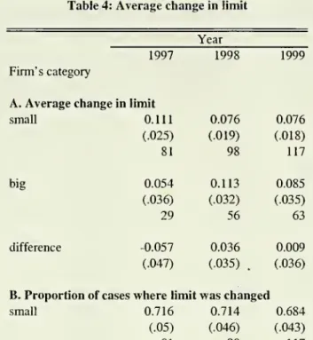
log(limit granted in year t-1). Table 4

shows

the average changein thecredit limit faced

by

the firm

between

period t

—

1

and

period t for 1997, 1998,

and

1999.

The

average

enhancement

was 5.7%

larger for small firms than for bigfirms

between

in 1997, whereas in 1998 it

was 3.6%

larger for big firms. In fact the size ofthe average

enhancement grew

for big firms

and

shrunk

for the small ones. In 1999, the size ofthe average

enhancement

was

almost exactly the

same

for small

and

large firms. This suggests that

banks

adjusted to the

change

in credit policy

by

raising the credit limit ofthe large firms once,

and

then placed

both

large

and

small firms

on

the

same

trajectory

Panel

B

intable4

shows

that theaverage increasein

enhancement

was

not

due

to

an

increase

in the probability that the working capital limit

was changed

: big firms did not

become

more

likely to experience achange in 1998 or 1999 thanin 1997. This

may

appear surprising, but it is entirely consistent with the previous evidence

showing

that it is not possible to explain

why

certain firms experienced a change in their credit limit. It is plausible that the

same

kind of

bureaucratic inertiais at

work

here as well.

While

loan officers

do

need to respond to pressure

from

the

bank

to

expand

lending to the

newly

eligiblebigfirms, they

seem

toprefergivinglarger

increases to those

which

would

havereceived

an

increase in anycase (for

one

reasonoranother)

,

rather than increasing the

number

of firms that receive enhancements.

InPanel C,

we

show

the average increaseinlimit, conditional

on

thelimit changing.

The

av-eragepercentage

enhancement was

23%

higher forsmall firms (andthisdifference issignificant)

.

It

was

3%

higher forthe large firms in 1998.

Our

strategy will be to use this change in policy as a source of shock to the availability of

bank

credit to these firms, using firms outside this category to control for possible trends.

The

first step

however

is to formally establish that there

was

indeed such a shock.

To

do

this

we

estimate an equation ofthe form:

logkut

-

logkbit-i

=

a

kb

BIGi

+

f3kb

POST

+

lkb

BIGi

*

POST

t

+

ekbiu (1)

where

kbit is a

measure

of

bank

credit to firm i in year t,

BIG

is a

dummy

indicating whether

the firm has investment in plant

and machinery between

Us. 6.5 millions

and

Rs. 30 millions,

and

POST

is a

dummy

equal to one in the years 1998

and

1999.

We

use a

number

ofdifferent

measuresof

banks

loans: working capitalloans

from

thisbank, total

working

capital loans

from

the

banking

sector,

and

total

term

loans. For

working

capital loans,

we

expect a positive 75.

We

do

notexpect achange in

term

loansin the years immediately following the reform, sinceit

takes

some

time for a fixed capitalinvestment project to be planned

and

processed.

As

pointed out in the previous subsection, the impact of the shock

on

the firm

depends

crucially

on whether

the firm

was

credit constrained, credit rationed or entirely unconstrained.

Inorder to distinguish

between

these cases

we

need tolook at a

number

ofothercredit variables

for the firm.

We

thereforerun a

number

ofother regressions that exactly parallel equation 1:

yu

-

Va-i

=

a

y

BIGi

+

(3

y

POST

t

+

ly

BIG

% *

POST

t

+

eyit, (2)

where yu

is a credit variable for firm i in year t. 12

• Credit rationing

Our

Result 1 above suggests that to establish credit rationing,

we

need

two

more

pieces of

evidence.

First, sincethe working capital loans take the

form

ofa line ofcredit (and firms are charged only for

what

they use),

we

need

to

examine

what

happened

to the rate at

which

firms

draw

upon

theirgranted limit.

We

thus use as our

measure

ofcredit utilization, the logarithm ofthe

ratioof turnover on accounts (the

sum

ofall debts overthe past year) to the credit limit.

Second, this

would

not

be

evidence ofcredit rationing ifthe interest rate charged

on

this

loan decreased at the

same

time. Priority sectors loans are not

supposed

to have lower interest

rates (the interest rate charged

on

a loan is the prime lending rate plus a

premium

depending

on

thecredit rating of thefirm-without regard forits status), sothere is

no prima

facie reason

the rate should fall. However,

we

directly check

whether

there is evidence ofthis using three

specifications: using

_y

it

—

r^in

equation (1) , forr^t equaltothe interestrate in logarithm

and

in level,

and

replacing

_yu

—

_yu-\ in equation (2)

by

a

dummy

indicating

whether

the interest

rate fell.

• Credit constraints

Credit rationing does not necessarily imply credit constraint.

To

investigate

whether

the

firms were credit constrained,

we

look at a

number

ofother pieces of evidence.

First, ifa firmwerecredit constrained, our theorytells usthat salesrevenue

would

definitely

go

up, while if it were not, sales should only go

up

forfirms that have already fully substituted

bank

credit for their

market

borrowing.

To

look at the effect ofcredit expansion

on

sales,

we

posit asimple parametric relation

between

credit

and

salesrevenue:

Ru

=

Aitk

u

.

Note

thatthis

Standarderrorsare correctedfor heteroskedasticity andclustering atthefirm andsector level.

isaspecific parametrizationofthe production functionintroducedinthe previous sub-section.13

log

Rn

=

log

A

it

+

log

ht

(3)

Differencingthis equation gives:

log Rit

-

\ogRit-i

=

log

A

it

-

log Ait-i

+

0[log

ku

-

logfcjt-i]. (4)

We

have already posited that the

growth

of

bank

credit is given by:

logfc_wt

-

logfcw,-!

=

a

kb

BIGi

+

(3_kb

POST

t

+

^

_kb

BIGi

*

POST

t

+

e kbit,

In theabsence ofcomplete substitution

between

bank

credit

and market

credit, this implies

a relationship of the

same

shape for capitalstock:

logku

-

log_ht-i

=

a

k

BIGi

+

(3_k

POST

t

+

7

_kb

BIG

t *

POST

t

+

ekit,

which

when

substituted in equation ₍₄₎ yields

log

Ru

-

logRit-!

=

log Ait

-

log

An^

+

0[ak

BIGi

+

P

k

POST

t

+

i

k

BIGi

*

POST

t

+

ekit]. ₍₅₎

Since

we

do

not observe log^4it

—

log^t-i

directly,

we

end

up

estimating an equation that

exactly

mimics

equation 2 above:

log^t

-

logife-!

=

a R

BIGi

+

f3

R

POST

t

+

lR BIGi

*

POST

t

+

v

kit]. (6)

Our

identificationhypothesis is that

log

A

it

~

log

Aa-!

=

a

A

BIG

l

+

(3

_A

POST

t

+

w«

, (7)

where

omegau

is uncorrelated with

BIG

*

POST.

This

amounts

to

assuming

that the rate of

change of

A

(whichis ashift parameter intheproduction function) did not changedifferentially

for big

and

small firms in the year of the policy reform.

Under

this assumption

_7^

gives the

reduced

form

effect ofthe

program on

sales revenue.

13

This is bestthought of asa reduced form, derived from a moreprimitive technology which makesoutput a

Cobb-Douglasfunction of theamountofn inputsx\,x?....xn. Aslong as theinputshave topurchased usingthe

working capitalandall inputs are purchasedin competitive markets, it can be shownthat the resulting indirect production function has theformgiven above.

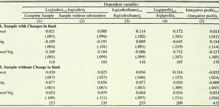
Iffirms arecredit constrained

7#

should

be

positive, while if

no

firms arecredit constrained

jR

will only

be

positive for those firms that havefully substituted

market

credit.

We

therefore

also estimateaversion ofequation 6 inthe

sample

offirms

whose

total current liabilities exceed

their

bank

credit. Ifthe firms

were

not creditconstrained, thevalue of

_7^

in this

sample

should

be

zero.

A

second strategy is to lookat substitution directly. Unfortunately

we

do

not have reliable

data

on market

borrowing.

We

therefore adopt the following strategy: equation (4)

above

can

be

rewritten in the form:

log Rit/kbit

-

log Rit-i/kbit-i

=

log

An ~

logAit-i

+9{\og ku

~

logfcft-i]

-

[logkbit

-

logkbit-i]. (8)

Differencing one

more

time gives us

[logRit/kbit -logRit-i/kbit-i]

-

[logRit-i/kbit-i

-log Ra-2/hu-2]

=

[log

An -

log Ait-i]

-

[logAit-i

-

log

An-2]

+0([log

ku/

kbit

-

logkit-i/kbit-i]

~

[logkit-i/kbit-i

-

logkit_2/kbit-2})

-(1

-

9)([logk^t

-

logkbit-i]

-

[logkbit-i

-

logkbit-2])- (9)

We

now

take the difference ofthis expression for big firms

and

that for small firms.

Denoting

by

the operator

A

theoperation ofdifferenceacross firm categories

and

using ₍₇₎

we

get

A{

[log

Rt/ht

-

logRt-i/ht-i]

-

[logRt-i/ht-i

-

logRt-

2

/k

bt-2]}

=

OA{([logkt/kbt

-

logkt-i/ht-i]

~

[logkt-i/kbt-i

-

logfct_2 /fcfct

_

2])}

-(1

-

9)A{[logk

bt

-

logkbt-!]

-

[loght-i

-

loght-2}}. (10)

We

have suggested,

and

will

show

formally

below

that A{[log

k

bt

—

logkbt-i]

—

[logkbt-i

—

logA;bt_2]} is positive

when we

compare

pre-reform

and

post-reform periods. If a firm is not

credit constrained it should substitute

bank

loans for

market

loans,

which

implies that

bank

capital should

grow

faster

than

total capital stockfor the big firms after the reform, relative to

the smallfirms. A{([log kt/kbt

-

logfct-iA&t-i]

-

[logfct-i/fcw-i

-

log

^-2/^-2])}

istherefore

negative.

As

long as 9

<

1, these

two

observations together imply that the expression

on

the right should

be

negative. If 9

>

1, this need not

be

necessarily be case, but with increasing

return to scale there cannot

be

an

equilibrium in

which

thefirms are not credit constrained.

We

implement

this

by

estimatingequation 2withy,t

=

^ Ifthe firmiscredit constrained,

7wk

hshould be negative. Ifnot,

we

presume

that there is

no

substitution.

A

final pieceofevidence

comes from

looking at profits.

Assuming

that the firm

buys

all its

inputs using its

working

capital,

we

can write

riit

=

Auikbit

+

k

_m

it)

9

-(1

+

rbi^kfct

-

(1

+

rmit)kmit

-

C.

It follows that

d\ogTijt

_{_}

A

it(kbit

+

kmit)

e

d\og

A

it 9Ait{kbit

+

kTnit)

e~1

kbi

t-{l

+

rbit)kbitd\ogkbit

dt

n

dt

n

dt

6

_Ag

(kbit

+

k

m

it) ~ k

m

jt

—

(1

+

T

m

ii)k

m

j t

dlogk

m

n

'Tmitkm.it

d\ogr

m

it

n

dt

n

dt '

ignoring the effect of changes in the

bank

interest rate, which, given evidence to

be

shown

later, does not

seem

tobe

much

of an issue. Ifthe firm

was

not credit constrained, kmit

would

be chosen optimally

and

therefore

we

can

drop

the third

term

in this expression.

Taking

time

derivatives again

and

droppingall termsthat involveaproductof

two

ratesofchange (assuming that rates of change are always small

and

therefore their products are going to be negligible),

we

get

rf2logII;t

_

Aujkbit

+

kmit)

e

d

2log

A

it

9A

u

{kbit

+

kmit) e~l

kbit

-

{\

+

rbit)kbit

d

2

\ogk

bi t dt2

n

dt2

n

dt2 rmitkmitdtlogrmit

n

dt2 '

Comparing

big

and

small firms,

and

invoking the

A

operator again,

we

have:

d

2

logn

t

A

t(kbt

+

k

m

t)°d

2 log

A

t

A

t(kbt

+

k

m

t) 9

d

2log

A

t , 1 dt2 ]

~

{

n

] dt2

+

_n

{ _dt2 _*

A

rr

m

tkmt~. d 2 logrmt

_

rmtfc_mt ri2logr_mt ^ 1

n

i dt2

n

{ dt2 j

9A

t{kbt

+

kmt) 9-l kbt

-

(1

+

rbt)kbt d 2 logkbt {

_n

dt2 } 16

Now

—

"^a""" should be the

same

for

both

large

and

small firms, since it is the

market

interest rate. Therefore

A{

d2'°^rmt

}

=

0.

By

equation 7 above,

A{

d2]°$At_}

=

0. Thisleaves us with:

d

2logIIt

_

A

t(kbt

+

kmt) e

d

2log

A

t { dt2 * x

n

* _dt2

[n)

A

,r

m

tkmt

d

2 logr_mt

9A

t{kbt

+

km

t) e-l kbt

-

(1

+

rbt)kbt d 2 logkbt {

n

] dt2

+

{

n

dt2 j '

The

last

term

here is the effect of the reform.

To

separate it

from

other time varying effects,

thefirst

two

terms

must be

small

enough

to

be

ignored.

The

second term,

A{

Tr

^^

nt }

d

'"^Z"""

can safely be

assumed

to be small. It has

been

shown

that, in India, the average interest rate

on

the internal

market

is linked to the

bank

rate.

—

_^/

mt is thus closely linked to

—

°^rt"

,

which

is given

by

the

POST

dummy

when

we

estimate equation (2) withrbt as the

dependent

variable. Below,

we

estimate this coefficient to

be

-0.16 percentage point (the average interest

rate is 14%).

One

scenario

where

/\{At{kbt

_^

krnt)<>}

d2l°

t%

At

is small is if

^$

At is small.

That would be

trueifeither there

was

not

much

changein At or ifthere

was

a directional trend but not

much

variation

around

the trend.

Assuming

that

A{

rmt

_£

mt}

d l

°$2mt is indeed small, this hypothesis

can

be

directly tested

by

looking at the coefficient of the

POST

dummy

when we

estimate

equation (2) withprofits asthe

dependent

variable: thecoefficient ofthe

POST

dummy

will

be

equal to

_^{

^k

ht+kmt)'

y

<P\^A

t

for the

smaU

firms gince

A

_^

A

t{kbt+kmt

)^

ig nQt equaJ tQ zer

_^

iftheproduct is zero,

—

°

ff

'

_{must be}

_zero.

Note

thatthe effectofthereformon profit is

due

to the

gap between

themarginalproduct of

capital

and

the bank interest rate: inother words, it combines the subsidy effect

and

thecredit

constraint effect: even iffirms were notcredit constrained, their profit

would

still increase after

thereformif

more

subsidized credit is

made

availabletothem, because they substitutecheaper

capital for expansive capital.

3.3

Empirical

Strategy:

Testing

the

Identification

assumptions

The

interpretation ofthe centralresult

on

sales

growth

crucially

depends

on

the

assumption

made

inequation (7). Likewise, the interpretation of the otherresults

depends on

the

assumption

that

theerror

term

isnot correlatedwith theregressors,

most

notably

BIG*POST.

However, there

are

many

reasons

why

this assumption

may

not hold. For example, big

and

small firms

may

be

differentlyaffected by other measuresof

economic

policy (theycould tendtobelong to different sectors, with different policies during these years). Moreover, being labeled as a priority sector

firm

may

have consequences for big firms over

and

above its effects

on

credit access.

There

are three other

ways

in which being included in the priority sector

may

affect firms. First, SSI

firms are

exempt from

some

types of excise taxation. Second, SSI firms

may

have better access

to

term

loans. Third, the right to manufacture certain products is reserved for the SSI sector.

We

will address the first concern

by

using profit beforetax,

and

the second

by showing

that in

the time span covered by our dataset, reform did not significantly affect

term

borrowing.

The

third concern could be a problem:

among

the small firms,

44%

manufacture a product that is

reserved for SSI.

Among

the big firms,

24%

do.

One

control strategy

would

be to leave out all

firms that manufacture products that are reserved for SSI. Unfortunately,

we

only

know

what

products the firm

manufactured

in 1998. It remains possible that

some

ofthe big firms

moved

into reserved products after 1998

and

this increased their profits.

As

a

way

totest ouridentificationassumption

and

to

improve

the precision of the estimates,

we

will estimate equation (2) for thedifferent

outcomes

variables separately using

two

samples:

the

sample

where

there

was no

change in the granted limit

from

oneyear to the next,

and

the

sample

where

there

was

a change (either an increase or decrease). In doing so,

we

make

use ofthe fact, noted above,

and

shown

more

formally below, that the probability ofa change in

the limit appears to be unaffected

by

the policy change (the variable

BIG

*

POST).

Given

this fact,

and

a simple monotonicity assumption, estimatingan equation ofthe

form

ofequation

(2) separately in the sample

where

there

was

a change in limit

and

in the

sample

where

there

was no

change in limit will lead to consistent estimates of the parameter of interest

₇

in

both

subsamples

(Heckman

(1979),

Heckman

and

Robb

(1986)).

Specifically, denote

q

a variable equal to 1 ifthere is a change in limit

and

otherwise, Zi

the interaction

BIG

*

POST,

and

Xi

the vector

(Bid,

POST).

Define en as the potential

selection status

when

Zi

=

1

and qo

as the potential selection status

when

Zi

=

0.14

Assume

that (i) (€i,{cn,Cio)) are jointly independent of Zi conditional

on Xi

(ii) one of the following

is true: conditional

on

Xi, en

>=

chq for all i or Cn

>=

chq for all i.

The

first assumption

guarantees the validity of Zi as a regressor in the complete sample (but not in the selected

For eachobservation, wewillobserve only eitherc,i or Cio

sample),

and

that the marginal distribution of

_qo

and

Qi (but not the joint distribution) are

identified in a

sample

with data

on

Zi

and

c*.

The

second

assumption

restricts the relationship

between

the instrument

and

selection to be monotonic: for all firms, the instrument

makes

it

either

more

likelyor less likely to experience a

change

inlimit.15

Given

these

two

assumptions, P(ci

=

\\Zi

=

1)

=

P(cj

=

l\Zi

=

0) implies that (ci,€i) is jointlyindependentof Zi conditional

on

Xi

(fora proofusingthis notation, seeAngrist _(1995)).

Therefore, E[ei\a

=

l,Zi

=

l,Xi]

=

E[ei\*

=

1,Z,

=

0,Xi],

and

E[ei\*

=

0,Zi

=

1,X

Z]

=

E[€i\ci

=

0,Zi

=

0,Xi\: the

OLS

assumptions are satisfied in

both

subsamples.

This implies that the independence

assumption

(which is equivalent to the assumption in

equation(7)can

be

tested as longasP(ct

=

l\Zi

=

1)

=

P(ci

=

l\Zi

=

0). Thislaterassumption

can inturn

be

shown

tohold

by

regressingthe probability ofa

change

in limit

on

the interaction

BIG

*

POST

(andfinding a coefficient ofzero

on

thisvariable).

The

test oftheidentification

assumption

is torun regressions ofthe

form

(2) in the

sample

with

no

increase in credit limit: since the coefficient ofthe variable

BIG

*

POST

iszero inthe

credit equation, it should also

be

zero in the regression of the other outcomes.

Of

particular

interest, obviously, arethe coefficients intheequation ofsales

and

profit. Ifthe firms are credit

constrained,

we

expect the coefficientsof

BIG

*

POST

to

be

positive inthe

sample

with credit

limit changes,

and

equal to zero in the

sample

with

no

changes in loans.

3.4

Empirical

Strategy: Structural

Estimates

The

fact that the firms are credit constrained tells us that the marginal product of capital is

higher

than

the

market

interest rate.

The

question is,

by

how

much?

We

begin

by

observing that

an

alternative to estimating equation (4) is to estimate the

structural relationship (4) using

BIGi

*

POST

t as

an

instrument.

16

This

would

allow us to

10

The latentindex formulation with alinearmodel Unkingthe latent variable to theinstrument satisfiesthese

two assumptions. However, the assumptions are not necessarilytrue: in particular,one could imagine thatthe limitfroma big firm ismorelikelytobeleft atzerothantobedecreased, butmorelikelytobeincreased thanto

be left at 0. Thiswould violate the monotonicity assumption.

We

will presentevidence belowthat this did not

seemtohave happened.

1

Following the discussion in the previoussubsection, we will run this IV regression in the samplewherewe

observean increasein loans.

estimate 6, the elasticity of revenue with respect to

working

capital investment. It is

worth

observing that for

an

equilibrium without credit rationing to exist it

must be

the case that

9

<

1 in theneighborhood ofthe equilibrium: otherwise the marginal product ofcapital is not

declining at the equilibrium,

which

rules out it being an

optimum

for

an

unconstrained firm.

Conversely, finding that 6

>

1,

makes

it likely that there arecredit constraints inequilibrium.

In practice, as

we

have already mentioned,

we

do

not have a

measure

of kit, but only a

measure

ofkbit- Rewriting structural equation (4),

we

obtain:

log Rtt

=

log

A

it

+

6logkbit

~

01og

_^|.

(12)

Differencingover time:

log

Ru

-logR.t-i

=

log

A

it

-

logAit-i

+

6(log

^

-logkbit-i)

-9[log~

~

]og

kti-l

^'

^

The

term

0[log

-^ —

logTjjrff],

which

is omitted in the regression, is positively affected

by

the

reform inthe presence of

any

substitution of

bank

credit for

market

credit. Thus,

when

we

use

Bid

*

POST

_t as

an

instrument for logfc^(,

we

obtain alower

bound

for 0.

The

expression

we

derivedfortheprofitrate

was

directlyexpressedasafunction of

difference-in-difference in the rate of changes of

bank

credit. Thus, to see

what

happens

to profit,

we

estimate the equation

log Rit

-

log

Rit^

=

aPOST

+

(3BIG

+

A[log kMt

-

log kba-i], (14)

using the interaction

POST*

BIG

as

an

instrument for [logkbit

—

logfe^t-i]-

Under

the

assump-tions in the previous subsection, A

=

e

M

k»t+ k

^)

e_-^k

bt-{i

+

rht)kbt _

Furthermore,

we

canuse the

assumption

that the probabilitythat the granted limit changes

is uncorrelated withthe interaction

BIG

*

POST

toconstruct

an

additional instrument,

which

will

make

use of the entire sample of firms to check for the robustness of our estimate: under

this assumption, the interactions

BIG

*

POST

and

BIG

*

POST

*

C

(where

C

is a

dummy

variable equal tooneifthere is

any

changein the limit) can

be

usedtogether as instrumentsfor

thechangesin limit inthe

outcomes

equations (aftercontrolling for

C

aswell asthe interactions

POST *C

and

BIG*

C).

4

Results

4.1

Credit

Expansion

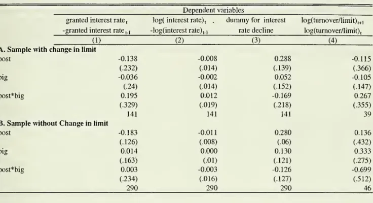
Table 5 presents the results of estimating equation (1) for several credit variables.17

We

start

with a variable indicating

whether

there is

any

was any change

in the granted limit (columns

(1)

and

(2)),

and two

dummies

indicating

whether

there

was an

increase or a decrease in the

granted limit. Consistent withthe evidence

we

discussed above, there

seem

to

be

absolutely

no

correlation

between

the probability to get

any

change at all,

any

increase or

any

decrease,

and

the interaction

BIG*POST.

Moreover, eventhe

main

effectsof

BIG

and

POST

areverysmall:

none

ofthe variables in this regression

seem

to affect

whether

the file

was

granted a change in limit or not. This is true

both

in the complete

sample

and

in the sample for

which

we

have

data

on

the next year's sale (which is smaller since

we

do

not use the last year of loan data).

In the following columns,

we

look at loans received

from

this

bank

(columns (5), (6)

and

(7)),

and

all working capital loans received

by

the

banking

sector (columns (8)).

As

the descriptive

evidencein table4 suggested, relativetosmall firms, loans

from

this

bank

to big firms increased

significantly faster after 1998

than

before: the coefficient of the interaction

POST

*

BIG

is 0.08, in the complete sample,

and

0.24 in the

sample

for

which

there is

any

change in limit.

Both

numbers

are significant. In

column

(6),

we

restrict the

sample

to observations that have a

changein credit limit.

There was

asignificantdecline intheaverage

enhancement

for small firms

(the

dummy

for

POST

is negative

and

significant). Before the expansionofthepriority sector,

small firmswere granted larger proportional

enhancement

than big firms (the coefficient ofthe

variable

BIG

in

column

(6) is -0.22, with a standarderror of0.079).

The

gap

completelyclosed

after the reform (the coefficient of the interaction is actually slightly larger in absolute value than the coefficient ofthe variable

BIG).

In

column

(7),

we

restrictthe

sample

to observations

where

we

have data

on

the next year's sales : the coefficient is almostthe

same

(0.23),

and

still

significant. In

column

(8),

we

look at the

sum

ofall credit received

from

the

banking

sector:

The

coefficient is alittle larger (0.295).

In

columns

(9)

and

(10),

we

lookin

more

detail atloans given

by

otherbanks: theprobability

1

Thestandarderrorsin all regressions are adjustedforheteroskedaticityandclustering atthe firmandsector

levels.