HAL Id: hal-02963289
https://hal.archives-ouvertes.fr/hal-02963289
Submitted on 10 Oct 2020
HAL is a multi-disciplinary open access
archive for the deposit and dissemination of
sci-entific research documents, whether they are
pub-lished or not. The documents may come from
teaching and research institutions in France or
abroad, or from public or private research centers.
L’archive ouverte pluridisciplinaire HAL, est
destinée au dépôt et à la diffusion de documents
scientifiques de niveau recherche, publiés ou non,
émanant des établissements d’enseignement et de
recherche français ou étrangers, des laboratoires
publics ou privés.
Distributed under a Creative Commons Attribution| 4.0 International License
Luc Dessart, Sung-Chul Yoon, David R. Aguilera-Dena, Norbert Langer
To cite this version:
Luc Dessart, Sung-Chul Yoon, David R. Aguilera-Dena, Norbert Langer. Supernovae Ib and Ic from
the explosion of helium stars. Astronomy and Astrophysics - A&A, EDP Sciences, 2020, 642, pp.A106.
�10.1051/0004-6361/202038763�. �hal-02963289�
Astronomy
&
Astrophysics
https://doi.org/10.1051/0004-6361/202038763
© L. Dessart et al. 2020
Supernovae Ib and Ic from the explosion of helium stars
Luc Dessart
1, Sung-Chul Yoon
2, David R. Aguilera-Dena
3,4, and Norbert Langer
3,41Institut d’Astrophysique de Paris, CNRS-Sorbonne Université, 98bis boulevard Arago, 75014 Paris, France
e-mail: [email protected]
2Department of Physics and Astronomy, Seoul National University, Gwanak-ro 1, Gwanak-gu, Seoul 151-742 Republic of Korea
3Argelander-Institut für Astronomie, Universität Bonn, Auf dem Hügel 71, 53121 Bonn, Germany
4Max Planck Institut für Radioastronomie, Auf dem Hügel 69, 53121 Bonn, Germany
Received 26 June 2020 / Accepted 14 August 2020
ABSTRACT
Much difficulty has so far prevented the emergence of a consistent scenario for the origin of Type Ib and Ic supernovae (SNe). Either the SN rates or the ejecta masses and composition were in tension with inferred properties from observations. Here, we follow a heuristic
approach by examining the fate of helium stars in the mass range from 4 to 12 M , which presumably form in interacting binaries. The
helium stars were evolved using stellar wind mass loss rates that agree with observations and which reproduce the observed luminosity
range of galactic Wolf-Rayet stars, leading to stellar masses at core collapse in the range from 3 to 5.5 M . We then exploded these
models adopting an explosion energy proportional to the ejecta mass, which is roughly consistent with theoretical predictions. We
imposed a fixed56Ni mass and strong mixing. The SN radiation from 3 to 100 d was computed self-consistently, starting from the input
stellar models using the time-dependent nonlocal thermodynamic equilibrium radiative-transfer code CMFGEN. By design, our fiducial
models yield very similar light curves, with a rise time of about 20 d and a peak luminosity of ∼1042.2erg s−1, which is in line with
representative SNe Ibc. The less massive progenitors retain a He-rich envelope and reproduce the color, line widths, and line strengths of a representative sample of SNe Ib, while stellar winds remove most of the helium in the more massive progenitors, whose spectra match typical SNe Ic in detail. The transition between the predicted Ib-like and Ic-like spectra is continuous, but it is sharp, such that
the resulting models essentially form a dichotomy. Further models computed with varying explosion energy,56Ni mass, and long-term
power injection from the remnant show that a moderate variation of these parameters can reproduce much of the diversity of SNe Ibc. We conclude that massive stars stripped by a binary companion can account for the vast majority of ordinary Type Ib and Ic SNe and that stellar wind mass loss is the key to removing the helium envelope in the progenitors of SNe Ic.
Key words. supernovae: general – radiative transfer
1. Introduction
Binary-star evolution has been recognized as an essential ingre-dient for the production of Type I core-collapse supernovae (SNe) since the 1980s (Wheeler & Levreault 1985; Wheeler et al. 1987;Ensman & Woosley 1988;Podsiadlowski et al. 1992;
Woosley et al. 1995;Vanbeveren et al. 1998;Wellstein & Langer 1999;Dessart et al. 2011;Smith et al. 2011;Langer 2012). This result was required to explain the frequencies of SNe Ibc (as well as SNe IIb), their short rise times to maximum light of about 20 d, and the narrow light-curve widths around bolometric max-imum (see for example the analyses of large samples byDrout et al. 2011,Taddia et al. 2015;Lyman et al. 2016, orPrentice et al. 2016,2019). This type of features are best explained by invoking low-mass ejecta, stemming from a low or moderate mass He star. An obvious progenitor of this scenario is therefore a 10−25 M
star in a binary system, which lost its H-rich envelope through an interaction with a companion (Eldridge et al. 2008;Yoon et al. 2010).
The He-star mass correlates with its luminosity, which con-trols the strength of the radiatively-driven wind at the origin of the subsequent wind mass loss (Langer 1989; Gräfener et al. 2011). For low He-core masses, the wind mass loss rate is weak and may not cause much mass loss at all. Being of low-mass and rich in He, the progenitor star may explode as a SN Ib or as a SN IIb if some residual H is present at the surface. Depending
on the mass loss rate, the winds of higher mass He-stars may or may not peel off the He-rich outer layers and produce a SN Ic, assuming that He deficiency is a prerequisite for a Type Ic classification (Liu et al. 2016).
For example, the mass loss rates used in the study ofYoon et al.(2010), which explored the stripped component of detailed binary evolution models, were too weak to produce the He-poor progenitors required for a Type Ic classification; these mass loss rate calibrations were taken fromHamann et al.(1982,1995), but scaled down by a factor 5 or 10. Indeed, out of 45 simulations, only two of their models are likely to make a Type Ic SN. Their lowest mass model produces a star at death of only 1.6 M , which
would produce an ultra-stripped SN Ic (Tauris et al. 2013). Their other models, for 12−25 M binary stars, which are favored by
the initial mass function and also suitable to produce low-mass He stars, would produce SNe Ib (or SNe IIb).
In the study of Yoon et al. (2010), not all binary parame-ters were explored. For example, the so called Case BB mass transfer after core He exhaustion is an efficient means to peel off the He-rich layers of a He star (Dewi et al. 2002;Dewi & Pols 2003). This type of mass transfer has been invoked to explain the Type Ic SN 1994I and its progenitor (Nomoto et al. 1994). This binary configuration is probably too rare to produce the majority of SNe Ic.
Recently,Yoon(2017) studied the evolution of He stars with mass loss. These He stars are expected to arise primarily from
A106, page 1 of16
interacting binaries. Yoon (2017) argued that the Wolf-Rayet (WR) mass loss rates that influence the subsequent evolution may have been underestimated. Indeed, higher WC mass loss rates appear essential to explain the sizable population of rela-tively faint WC stars (Sander et al. 2012). The mass-luminosity relation during He-core burning (Woosley 2019) implies that these fainter WC stars must be of a lower mass than previously predicted. A reduction in the final mass of WC stars (at least for a subset of these stars) could help resolve the mass discrepancy that currently holds between the high WC star masses at death (see discussion and references inYoon 2017) and the relatively low SNe Ic ejecta masses inferred from observations.
Much debate has taken place over the last decades on the pos-sibility of hiding He, and in particular below what threshold He mass HeIlines would be invisible (Swartz et al. 1993;Dessart et al. 2012;Hachinger et al. 2012). Unfortunately, the detection of HeI lines in SN spectra is often hard to secure, and this is not limited to SNe Ibc since the problem also affects Type II SNe. Typical SN II-P show at best a weak HeI5876 Å line at
early times, but as soon as the recombination phase starts, HeI
lines are absent in the optical, even though He makes about 35% of the H-rich envelope mass. Evidently, several solar masses of He go un-noticed in garden-variety SNe II-P. In these SNe II-P, it is the presence of H (essentially at a level set by Big-Bang nucleosynthesis) that implies indirectly the presence of He.
In stripped-envelope core-collapse SNe, the situation is dif-ferent. In rare instances, SNe IIb or Ib show a similar blue optical color at early times to what is observed in SNe II-P (e.g., SNe 1993J or 2008D; Matheson et al. 2000; Soderberg et al. 2008;Modjaz et al. 2009), indicative of a large gas temperature suitable for the production of HeIlines through photoionization
and recombination. Unfortunately, these blue optical spectra are also quasi-featureless so that HeIlines are not evidently present.
Instead, HeI lines are seen at the recombination epoch, when
the SN radiation peaks in the optical and the SN photospheric temperature is around 7000 K. Under such conditions, the pro-duction of HeIlines requires nonthermal excitation (Lucy 1991; Swartz 1991). This process is controlled by the amount of56Ni
and the mixing of 56Ni in velocity space (Dessart et al. 2012).
The mass fraction of He is also a fundamental quantity since the decay power (and the associated nonthermal rates) scales with the species’ abundance. So, if a given mixture contains 10% of He, only 10% of the decay power will go to He atoms. Hence, not only the low abundance of He disfavors the production of strong HeI lines, but the sharing of the decay power between species
also means that nonthermal rates affecting He will also be low. In contrast, if the He mass fraction is 90% or more, not only the large He abundance fosters the production of strong lines, but He also absorbs nearly the entire decay power, favoring the nonthermal excitation of HeIlines (Dessart et al. 2012).
Observations present further biases and challenges. Line overlap (for example of NaID with HeI5876 Å) implies that
most observed features are blends of multiple lines. Weak lines are also hard to detect unless the signal-to-noise ratio is high. Fast expansion and the associated Doppler broadening yields weaker lines more likely affected by overlap with lines from other atoms or ions. Despite all these difficulties, numerous SNe exhibit strong HeIlines. Notorious HeIlines in the optical are
at 5876, 6678, and 7065 Å (for example in the CfA sample, SNe 2004gq, 2004gv, or 2005hg;Modjaz et al. 2014), but other HeI lines in the blue part of the optical are also predicted and
observed (seeDessart et al. 2011and below). When an ambiguity on He detection arises, it concerns objects in which the HeIlines
are weak, and sometimes vanishingly so. Hence, there is a clear dichotomy amongst Type I SNe from massive star explosions, with events showing strong HeIlines and all the rest.
Massive star evolution predicts the presence of He even in the most evolved WR stars (see, for example, Meynet et al. 1994), and the observations of these stars confirms this (see, for example,Kingsburgh et al. 1995;Crowther et al. 2000). But the separation of observed WR stars between WN stars (atmospheric composition inferred to be rich in He and N, with a He mass fraction of 90% or more;Crowther et al. 1995a,b) and the WC stars (atmospheric composition inferred to be rich in C and O, with a He mass fraction at the 10% level;Koesterke & Hamann 1995;Grafener et al. 1998;Hillier & Miller 1999;Crowther et al. 2002;Sander et al. 2012) offers a possible explanation for a strict dichotomy between SNe Ib and Ic. The surface composition of observed WC stars also suggest that the absence of He is not expected, and perhaps not required (to produce a SN Ic), in any massive star at core collapse.
In this work, we focus on “standard” SNe Ibc, or what pro-genitors and explosions produce the majority of SNe Ibc. We present radiative transfer simulations of He-star explosions that, for the first time, match the properties of the majority of SNe Ibc, reproducing simultaneously their light curves out to ∼100 d and their spectra around maximum light. Rather than fitting one specific event, we aim to produce models that overlap with the parameter space occupied by such standard SNe Ibc and that reproduce the observed dichotomy between the SN classification as Type Ib or Ic. These SN simulations are based on a physi-cally consistent set of stellar-evolution calculations for He stars, made to approximately mimic the evolution of previously H-rich stars that most likely lost their H-rich envelope by binary mass exchange. Unlike all previous studies, we address the suitability of the models both against the photometric properties and the spectroscopic properties using nonlocal thermodynamic equi-librium (nonLTE) time-dependent radiative transfer calculations that encompass the ejecta evolution from 3 to 50–100 d after explosion.Woosley(2019) andErtl et al.(2020) performed sim-ilar simulations for the evolution and explosion of He stars (with a number of differences in the approach) but these were limited to the computation of SN bolometric light curves and a coarser comparison to observations than presented here.
In the next section, we present the numerical approach for computing our stellar evolution models, the explosion mod-els, and how we follow the evolution of the SN radiation with nonLTE time-dependent radiative transfer. We then describe the light curve (Sect.3) and the spectral (Sect.4) properties of our ejecta models. In Sect. 5, we confront our model results to a selection of observed SNe Ib and Ic. In Sect.6we discuss the ori-gin of some degeneracies in the modeling of SNe Ibc. In Sect.7, we present our conclusions and discuss the implications of our results on the understanding of SNe Ib and Ic.
2. Numerical approach
2.1. Stellar evolution until core collapse with MESA
Our calculations started with pure He-star models with initial masses in the range 4 to 12 M , which were evolved in time using
the MESA code (Paxton et al. 2011, 2013, 2015, 2018, version 11 554). We implicitly assume that these stars stem from 14– 32 M main sequence stars, and that their hydrogen envelopes
have been completely removed by a binary companion once core He burning begins. Detailed binary evolution models show that mass transfer due to Roche-lobe overflow does remove most but
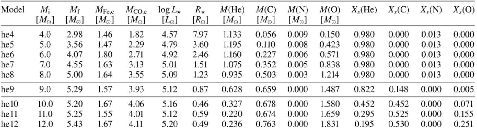
Table 1. Properties of our set of progenitor models.
Model Mi Mf MFe,c MCO,c log L? R? M(He) M(C) M(N) M(O) Xs(He) Xs(C) Xs(N) Xs(O)
[M ] [M ] [M ] [M ] [L ] [R ] [M ] [M ] [M ] [M ] he4 4.0 2.98 1.46 1.82 4.57 7.97 1.133 0.056 0.009 0.150 0.980 0.000 0.013 0.000 he5 5.0 3.56 1.47 2.29 4.79 3.60 1.195 0.110 0.008 0.423 0.980 0.000 0.013 0.000 he6 6.0 4.07 1.80 2.71 4.92 2.46 1.160 0.227 0.006 0.571 0.980 0.000 0.013 0.000 he7 7.0 4.55 1.63 3.13 5.01 1.51 1.075 0.352 0.005 0.838 0.980 0.000 0.013 0.000 he8 8.0 5.00 1.64 3.55 5.09 1.23 0.935 0.503 0.003 1.214 0.980 0.000 0.013 0.000 he9 9.0 5.29 1.57 3.93 5.12 0.87 0.628 0.659 0.000 1.487 0.822 0.148 0.000 0.005 he10 10.0 5.20 1.67 4.06 5.16 0.46 0.327 0.678 0.000 1.580 0.452 0.452 0.000 0.071 he11 11.0 5.25 1.55 4.01 5.12 0.59 0.220 0.674 0.000 1.659 0.295 0.525 0.000 0.155 he12 12.0 5.43 1.67 4.11 5.20 0.49 0.236 0.763 0.000 1.831 0.195 0.530 0.000 0.251
Notes. Models he4-he8 (he10-he12) correspond to SNe Ib (Ic) progenitors. Model he9 is an intermediate case. For each progenitor model, the
table gives the initial mass Mi, the final mass Mf, the Fe-core mass (where the electron fraction first rises to 0.499 from the center), the CO-core
mass (outermost location where the He mass fraction is lower than 0.01), the final surface luminosity log L?, the final surface radius R?, followed
by the total mass of He, C, N, O, as well as the surface mass fraction of He, C, N, and O.
not all of the hydrogen envelope (Gilkis et al. 2019). However, for the metallicity and mass range considered here, the assump-tion that the ensuing strong stellar wind blows off any remaining hydrogen within a short time remains a good approximation (Laplace et al. 2020). Notably, we did not consider the lowest mass helium stars that could still produce SNe despite their low mass, and that may (Yoon et al. 2010) or may not (Antoniadis et al. 2020) retain their hydrogen.
Whereas for the lower mass He stars considered here, a sin-gle star origin appears unlikely, it cannot be excluded that sinsin-gle stars with initial masses near 30 M may lose their envelope
quickly after core hydrogen exhaustion (Smith & Owocki 2006;
Petrov et al. 2016). Corresponding single stars would produce the same SNe as we predict from our He star models, and merely augment their number. Possibly, some single stars in the upper part of the mass range considered here evolve into red super-giants, where stellar wind mass loss may remove most of the H-rich envelope during core helium burning. The winds during the ensuing WR stage may or may not remove the remaining hydrogen and helium layers. This would lead to larger final masses (Woosley 2019), some of which may form black holes (Langer et al. 2020) or Type IIb SNe (Claeys et al. 2011). While these objects may contribute to the diversity of stripped enve-lope SNe, in view of the prevalence of binarity for massive stars (Sana et al. 2012) we consider binary evolution to be the favored scenario for the formation of our initial He star models.
The initial chemical composition of our models was set to mimic the He-core composition at the end of the main sequence of a 25 M star: X(4He) = 0.98, X(12C) = 3.40 × 10⁻⁴,
X(14N) = 1.30 × 10⁻², X(16O) = 3.4 × 10⁻⁴. Elements that are not
affected by H burning have the standard values ofGrevesse & Sauval (1998) at a metallicity Z = 0.02. The CNO equilibrium abundances would somewhat differ for different temperatures and hence for different He-star masses, but this detail is not important for our purpose. We adopted the Schwartzschild crite-rion for convection with a mixing-length parameter of two. We assumed no overshooting. Nuclear burning was treated with the network approx21.net. All simulations were evolved until the maximum infall velocity of the iron core reaches 1000 km s−1.
For the mass loss rate of such He stars, we followed the pre-scription by Yoon(2017), which distinguishes mass loss rates from WN and WC/WO type stars, and has a simple interpolation between the two. The adopted WN mass loss rate is based on the
study of LMC WN stars byHainich et al.(2014) and includes a scaling by Z0.5
. The WC and WO mass loss rates are based on the
study ofTramper et al.(2016). This mass loss rate is significantly higher than the WN mass loss rate for a given luminosity, which tends to exacerbate the composition contrast between WN and WC stars at the pre-SN stage. The stellar wind parameter fwwas
set to 1.6, which corresponds to a wind clumping factor of four ( fw=1.0 corresponds to a wind clumping factor of 10). We find
that fw=1.6 can reproduce the luminosity distribution of WN
and WC stars in our Galaxy and the LMC (Yoon 2017).
Our simulations were performed for He stars with an initial mass covering from 4 to 12 M in 1 M increments. The model
nomenclature is such that heM refers to the He star model with an initial mass of M M . Table 1 gives a summary of
prop-erties for each of these models at the onset of core collapse. Figure1 illustrates the density stratification, and the composi-tion profile for He and O versus Lagrangian mass. In this model sequence, the surface helium abundance and the He-rich shell mass decrease in favor of a growing surface C/O abundance and CO core mass. The final star mass grows from 2.98 (he4 model) up to 5.43 M (he12 model), thus producing lower final masses
than previously obtained with alternate mass-loss prescriptions. As discussed byYoon(2017), these models also produce faint WC stars at death, with log L? in the range 4.6−5.2. The final
mass and luminosity of these models appear similar to those ofErtl et al.(2020) for their “1.5 × ˙M” prescription (see their Table1).
Our models were evolved at solar metallicity. Metallicity might play a role, though probably secondary, in the evolution of binaries, and thus in the formation of stripped-envelope stars (Gilkis et al. 2019;Laplace et al. 2020;Shenar et al. 2020). How-ever, metallicity will probably influence primarily the WR mass loss rate so that higher metallicities will favor the production of SNe Ic relative to Ib (Georgy et al. 2009). Although there is no strong metallicity dependence affecting the number ratio of SNe Ibc versus SNe II, SNe Ic seem to be more prevalent than SNe Ib at higher metallicity (Modjaz et al. 2011;Anderson et al. 2015). 2.2. Radiation-hydrodynamics simulations of the explosion
with V1D
The progenitor models described in the previous section were used as initial conditions in the radiation hydrodynamics code
Table 2. Properties of ejecta models produced from the set of progenitor
models presented in Sect.2.1and Table1.
Model Mej Ekin Vm 56Ni0 Epm [M ] [1051erg] [km s−1] [M ] [1049erg] he4 1.49 0.75 7117 0.08 · · · he5 2.01 1.02 7134 0.08 · · · he6 2.37 1.21 7152 0.08 · · · he7 2.85 1.46 7187 0.08 · · · he8 3.31 1.67 7135 0.08 · · · he9 3.59 1.81 7119 0.08 · · · he10 3.39 1.77 7239 0.08 · · · he11 3.56 1.77 7068 0.08 · · · he12 3.67 2.11 7608 0.08 · · · he4 1.49 0.75 7117 0.08 · · · he4epl 1.49 1.63 10 504 0.08 · · · he4ep 1.49 1.64 10 509 0.16 · · · he4pml 1.49 0.75 7118 0.08 1.0 he4pmu 1.49 0.75 7124 0.08 2.0 he9 3.59 1.81 7119 0.08 · · · he9pml 3.59 1.81 7121 0.08 1.0 he9pmu 3.59 1.81 7123 0.08 2.0 he12 3.67 2.11 7608 0.08 · · · he12epl 3.68 4.77 11 414 0.08 · · · he12ep 3.69 4.76 11 396 0.16 · · · he12pml 3.67 2.11 7604 0.08 1.0 he12pmu 3.67 2.11 7605 0.08 2.0 he12eppml 3.68 4.76 11 409 0.16 1.0
Notes. For models with a suffix pml and pmu, the magnetar field is
1015G.
V1D (Livne 1993; Dessart et al. 2010b,a). Unlike Ertl et al. (2020), we did not follow self-consistently the neutrino-driven explosion so that our explosion energies (as well as power ver-sus time or mass cut) were prescribed rather than obtained from first principles (the explosion is still designed at some level in the 1D simulations ofErtl et al. 2020). Immediately above the outer edge of the iron core (which increases from about 1.5 to 1.8 M
from model he4 to model he12), we initiated a thermal bomb by depositing energy in the innermost 0.05 M for a duration
of 0.2 s. The total energy deposited that we prescribed corre-sponds to the envelope binding energy plus an energy per unit ejecta mass of 5 × 1050erg M−1
. With this scaling, we aimed
to produce ejecta for models he4 to he12 that had the same Ekin/Mej. Our values of Ekinare representative of those obtained
in the more realistic simulations ofErtl et al.(2020) and typical of what may obtain in core collapse SNe like 1987A (Arnett et al. 1989).
Explosive nucleosynthesis is very sensitive to the position of the mass cut, the core density structure, the power and the total energy of the explosion so the56Ni mass differs between our V1D
simulations. Since our explosion setup is artificial, we took the freedom to reset the56Ni mass to be 0.08 M
in all models at
10 s after the explosion trigger. Having a fixed56Ni mass in this
he4–he12 sequence facilitates the comparison between models. It was motivated also by the desire to reproduce the properties of garden-variety SNe Ibc, whose light curves are often undis-tinguishable (Drout et al. 2011). For simplicity, we kept the same
0.0 0.5 1.0 1.5 2.0 2.5 3.0 3.5 4.0 4.5 5.0 5.5 m [M ] −12 −−10 8 −6 −4 −2 0 2 4 6 8 10 log ( ρ / g cm − 3) he4 he5 he6 he7 he8 he9 he10 he11 he12 0.0 0.5 1.0 1.5 2.0 2.5 3.0 3.5 4.0 4.5 5.0 5.5 m [M ] 0.0 0.2 0.4 0.6 0.8 1.0 X ( 4He ) he4 he5 he6 he7 he8 he9 he10 he11 he12 0.0 0.5 1.0 1.5 2.0 2.5 3.0 3.5 4.0 4.5 5.0 5.5 m [M ] 0.0 0.2 0.4 0.6 0.8 1.0 X ( 16O ) he4 he5 he6 he7 he8 he9 he10 he11 he12
Fig. 1.Properties of our set of He-star progenitor models he4 − he12 at the onset of core collapse. Top panel: density structure, followed by the He and O mass fraction, all shown versus Lagrangian mass.
nomenclature for these nine ejecta models as for the nine pro-genitor models, that is to say we sticked to he4 to he12 (variants of this reference set of explosion models will be given the same root name with an additional suffix).
The ejecta mass Mej(which is just Mf− MFe core; our models
experience no fallback) increases monotonically in our he4–he12 model sequence from 1.5 to 3.6 M . Since the same power per
unit mass was used in our approach, the ejecta kinetic energy increases from 0.75 to 2.1 × 1051erg in the he4–he12 model
set (variations occur because of the nuclear energy released by explosive burning, which is greater in higher mass progenitors). The mean ejecta velocity Vm=p2Ekin/Mejis about 7200 km s−1
for all models. Our ansatz is that higher mass progenitors explode with a higher energy and yield a higher ejecta kinetic energy at infinity (despite the growing binding energy of their core). This correlation is supported by the simulations ofErtl et al.(2020) but only up to He core masses of about 6 M . We assume that it
holds all the way to our most massive progenitor model he12. In all simulations, some56Ni mixing was enforced by using a
boxcar with a width set to Mej/3. Since the model sequence he4–
he12 is also characterized by the same Ekin/Mej, models he4 to
he12 have the same 56Ni profile in velocity space, modulo an
offset in magnitude due to the difference in Mej. In other words,
X(56Ni) × M
ejis the same for models he4 to he12. This mixing
is therefore strong in all our models, bringing56Ni all the way to
the outermost ejecta layers. The short rise times and large peak luminosities of SNe Ibc suggest that weak mixing is unlikely in SNe Ibc. Simulations for varying levels of mixing have been presented earlier (Dessart et al. 2012,2015; see alsoYoon et al. 2019).
As discussed in a number of recent papers, explaining the SNe Ibc brightness during the photospheric phase or early neb-ular phase exclusively by56Ni decay power requires a56Ni mass
that is on average larger than for SNe II (Drout et al. 2011;Lyman et al. 2016;Prentice et al. 2016,2019;Meza & Anderson 2020;
Sharon & Kushnir 2020). In the simulations ofErtl et al.(2020), the56Ni mass is typically below 0.1 M
and thus in tension with
the value inferred for about half of SN Ibc observations. Part of this tension arises from a few outliers with erroneous estimates of the56Ni mass, for example because of an overestimate of the
reddening (e.g., SN 2005hg claimed byLyman et al. 2016to have 0.66 M of 56Ni but this estimate relies on an adopted
redden-ing E(B−V) of 0.685 mag, when in fact the reddenredden-ing is low and probably about 0.1 mag – see below). However, even with-out these with-outliers, an offset remains in the distribution of 56Ni
masses between SNe Ibc and SNe II-P (Anderson 2019;Meza & Anderson 2020).
Although the main focus of the paper was on reproducing the properties of the majority of SNe Ibc at the lower end of the peak-luminosity distribution, we also investigated possible causes for more luminous SNe Ibc. Indeed, the neutrino mecha-nism of core-collapse explosion of He stars yields SN ejecta that asymptote to a peak luminosity of about 1042.2erg s−1(Ertl et al. 2020), while standard SNe Ibc are observed with inferred peak luminosities up to about 1042.6erg s−1. For these more luminous
SNe Ibc, we tried various options including increasing the ejecta kinetic energy only, increasing both the ejecta kinetic energy and the56Ni mass, and finally injecting power from the compact
rem-nant. This power may originate from fallback accretion (see for example Dexter & Kasen 2013) or from dipole-radiation by a magnetized and rotating neutron star (see for exampleKasen & Bildsten 2010) – see also discussion inErtl et al.(2020). Both processes have a similar time dependence, in particular at late times of weeks to months (as 1/t5/3 for fallback compared to
1/t2for dipole radiation from a magnetar). For the same energy
input, both processes may thus yield a similar impact on the SN ejecta and its radiation. For practical reasons (magnetar power is implemented in CMFGEN;Dessart 2018), we parametrized some simulations with a power from a slowly rotating magnetar.
For these variants, we thus considered the following addi-tional models. In models he4ep (he12ep), the total energy deposited and the enforced56Ni mass are twice that in model he4
(he12). In models he4epl (he12epl), the total energy deposited is twice that in model he4 (he12), but the56Ni is left at 0.08 M
.
For models he4, he9, he12, two additional variants were done for
each by including magnetar power with Bpm=1015G and either Epm=1049erg (model with suffix pml) or Epm=2 × 1049erg
(model with suffix pmu). The magnetar with the characteris-tics “pml” given above was also included in model he12eppml, which is otherwise the same as model he12ep.
2.3. Time dependent nonlocal thermodynamic equilibrium radiative transfer with CMFGEN
Using the set of ejecta models produced with V1D and described in the previous section, we solved the nonLTE radiative trans-fer problem with CMFGEN (Hillier & Miller 1998; Dessart & Hillier 2005;Hillier & Dessart 2012). We started the CMFGEN simulations at about 3.5 d after explosion since we wished to focus on the epochs around maximum. Most simulations were stopped at 70 d after explosion, while a few were continued until 100−150 d to track the late-time brightness evolution indicative of the magnitude of γ-ray escape. Metals not treated in the net-work approx21.net during the pre-SN evolution were given an abundance at the solar metallicity value.
We treated nonthermal processes as per normal (Dessart et al. 2012;Li et al. 2012). We limited the radioactive decay to the56Ni chain. For simplicity, we computed the nonlocal energy
deposition by solving the radiative transfer equation with a gray absorption-only opacity to γ-rays set to 0.06 Yecm2g−1, where
Yeis the electron fraction.
The model atom includes HeI (40,51), HeII (13,30), CI
(14,26), CII(14,26), NI(44,104), NII(23,41), OI(19,51), OII (30,111), NeI(70,139), NeII(22,91), NaI(22,71), MgI(39,122), MgII (22,65), AlII (26,44), AlIII (17,45), ScI (26,72), ScII (38,85), ScIII(25,45), SiI(100,187), SiII(31,59), SiIII(33,61), SI (106,322), SII (56,324), SIII (48,98), ArI (56,110), ArII (134,415), KI(25,44), CaI(76,98), CaII(21,77), TiII(37,152), TiIII(33,206), CrII(28,196), CrIII(30,145), CrIV(29,234), FeI (44,136), FeII(275, 827), FeIII (83, 698), FeIV(51,294), FeV (47,191), CoII (44,162), CoIII (33,220), CoIV (37,314), CoV (32,387), NiII(27,177), NiIII(20,107), NiIV(36,200), and NiV
(46,183). The numbers in parenthesis correspond to the num-ber of super levels and full levels employed (for details on the treatment of super levels, seeHillier & Miller 1998).
When comparing to observations, we consider the quasi-bolometric light curves out to 50−100 d after explosion but we analyze the spectral properties at one epoch, early after bolo-metric maximum. Spectra at that time are usually available in SNe Ibc (see for exampleModjaz et al. 2014). Starting at or early after maximum light, the influence of the progenitor structure, and in particular whether the progenitor is compact or extended, has abated so the spectral properties are primarily sensitive to composition (56Ni and other elements). The mixing of 56Ni is
also less important since the γ-ray mean free path is longer, even for weak mixing (Dessart et al. 2015). The full ejecta is turning optically-thin in the continuum so that the spectrum forms over the full ejecta, allowing a probe of most of the ejecta mass (the outermost fast expanding layers of the ejecta are optically thin at this time but they contain very little mass and thus bear less sig-nificance for understanding the progenitor star composition and mass).
2.4. Differences with previous simulations of SNe Ibc with CMFGEN
Simulations of SNe Ibc have been performed in the past with CMFGEN (Dessart et al. 2011, 2012, 2015, 2016, 2017) and so
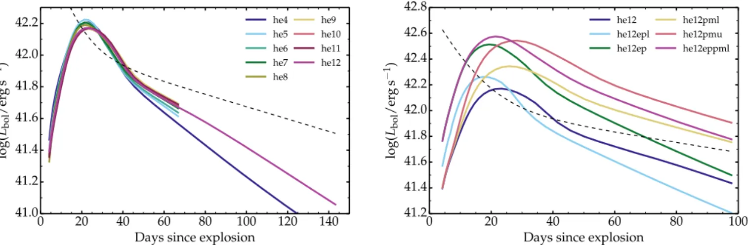
0 20 40 60 80 100 120 140 Days since explosion
41.0 41.2 41.4 41.6 41.8 42.0 42.2 log( Lbol /er g s − 1) he4 he5 he6 he7 he8 he9 he10 he11 he12 0 20 40 60 80 100
Days since explosion 41.2 41.4 41.6 41.8 42.0 42.2 42.4 42.6 42.8 log( Lbol /er g s − 1) he12 he12epl he12ep he12pml he12pmu he12eppml
Fig. 2.Left: bolometric light curves computed with CMFGEN for the explosion models based on He-star models he4 to he12. All nine models have
the same56Ni mass of 0.08 M
and the same ejecta kinetic energy per unit mass of 5 × 1050erg M−1 . Right: bolometric light curves for model he12
and variants that include power from the compact remnant (he12pml and he12pmu), a higher kinetic energy (he12epl), a higher kinetic energy and
higher56Ni mass (he12ep), and both combined (he12eppml). Details on these ejecta model parameters are given in Table2. In both panels, the
dashed line gives the instantaneous decay power emitted by an initial56Ni mass of 0.08 M
.
it might be useful to clarify what distinguishes these various studies. In the first four studies, we used a selection of binary progenitor models from Yoon et al. (2010). In Dessart et al.
(2011), the selection was augmented to include single-star mod-els. InDessart et al.(2017), only single star models were included (all based on a 40 M progenitor star, often with allowance for
rotation), and the study was more focused on highly energetic explosions leading to SNe Ic-BL and GRB/SNe Ic. In the present work, we start with He star models, which most likely arise from binary evolution. In contrast, the models fromYoon et al.(2010) were evolved consistently from the ZAMS in a binary system. Our progenitor models were computed with MESA while those of Yoon et al. (2010) were computed with the code BEC and KEPLER. Finally, the mass loss prescriptions differ significantly for the WR stage. InYoon et al.(2010), the mass loss rate cali-brations were taken fromHamann et al.(1982,1995), but scaled down by a factor 5 or 10, which tended to produce massive WC stars at core collapse. In the present study, the WR mass loss rates are greater (see Sect. 2.1 andYoon 2017). Furthermore, in the models of Yoon et al. (2010), WR mass loss rate were a function of luminosity (and hydrogen mass fraction, which is irrelevant for the present He-star models) and did not consider the difference between WN and WC/WO stars. Therefore the amount of He at the pre-SN stage was a smooth function of the progenitor mass, in contrast with the progenitor models produced in this work.
The treatment of the explosion in these studies is compara-ble, irrespective whether the code used was KEPLER or V1D. A small or moderate-size nuclear network was employed (account-ing for 21 up to 71 isotopes). The explosions were generated artificially, either with a piston or a thermal bomb. Given the focus of our present and past studies, only the total explosion energy and56Ni mass matter.
An important difference between these studies is the treat-ment of nonthermal processes in CMFGEN. These were ignored in
Dessart et al. (2011), so that model spectra were only accurate as long as 56Ni decay did not influence the spectrum
forma-tion region. This prevented the discussion of the model spectra after about a week past explosion. From 2012 onward, non-thermal processes were treated so that the nonLTE physics was accurately handled (for example with respect to the presence or
absence of HeI lines). The treatment of radioactive decay was
flexible from the start. We have been using local (when the γ-ray mean free path is very small) or nonlocal energy deposition. For the latter, a Monte-Carlo technique was used until 2016 to transport γ-rays. Since then, we have been solving the gray pure-absorption radiative-transfer equation for the γ-rays. The Monte Carlo method is a little more accurate but the second method is more convenient and faster (see discussion inWilk et al. 2019).
Based on our experience, the decisive difference between this work and previous studies of SNe Ibc with CMFGEN is the use of a new set of progenitor models. Specifically, it is the revision of WR mass loss rates affecting our He star models, most likely produced from binary evolution, that brings the possibility of explaining the properties of standard SNe Ibc. This is the central motivation for the present work.
3. Results: light curve properties
Figure2 shows the bolometric light curve for a subset of our models. Not all models are shown since there is a lot of degen-eracy, but the main light curve characteristics are given in Table3. In this table, we provide the rise time to maximum, the UVOIR luminosity or V-band magnitude at maximum, and the brightness decline between the time of maximum and 15 days later.
The left panel of Fig. 2 shows that the choice of a fixed value of 5 × 1050erg M−1
for the ejecta models he4–he12 yields
essentially the same light curve properties up to about 40 d after explosion. This emphasizes again the degeneracy of SN Ibc light curves and the difficulty of constraining the ejecta mass or kinetic energy. The rise time to bolometric maximum ranges between 18.2 and 24.4 d. The rise time to V-band maximum occurs a little earlier and is between 17.8 and 22.4 d. The bolo-metric luminosity peaks between 1.46 and 1.68 × 1042erg s−1
(corresponding to the range 42.16 to 42.2 in the log). Lighter models tend to peak earlier, at a larger luminosity, and decline faster both early after maximum as well as at all times in the nebular phase. These differences are however small.
Drout et al.(2011) found that their sample of SNe Ib and Ic had light curve properties that were statistically undistinguish-able from each other. The left panel of Fig.2shows that realistic
Table 3. Properties of the UVOIR and V-band light curves for the full model set, including the rise time to maximum, the peak luminosity or magnitude, and the decline in brightness between the time of maximum and 15 days later.
Model LUVOIR V Tph Vph ∆MV>Vph X(He)ph X(O)ph
trise Max ∆M15 trise Max ∆M15
[d] [1042erg s−1] [mag] [d] [mag] [mag] [K] [km s−1] [M ] he4 23.0 1.60 0.68 22.4 −17.12 0.82 6448 8394 0.36 0.94 0.00 he5 22.2 1.68 0.69 21.4 −17.17 0.84 6355 8896 0.39 0.93 0.00 he6 22.4 1.61 0.63 21.7 −17.15 0.82 6287 8819 0.48 0.85 0.02 he7 22.2 1.60 0.59 21.1 −17.15 0.70 6335 8637 0.60 0.70 0.06 he8 22.5 1.55 0.50 21.1 −17.10 0.59 6220 8617 0.65 0.57 0.07 he9 23.7 1.46 0.42 21.7 −17.06 0.50 6035 8297 0.80 0.33 0.17 he10 23.5 1.49 0.50 21.6 −17.12 0.59 6022 8427 0.76 0.18 0.28 he11 24.4 1.48 0.50 22.2 −17.09 0.59 6000 8344 0.76 0.11 0.39 he12 23.5 1.48 0.50 21.5 −17.12 0.58 5920 8758 0.86 0.11 0.37 he4 23.0 1.60 0.68 22.4 −17.12 0.82 6448 8394 0.36 0.94 0.00 he4epl 18.2 1.76 0.87 17.8 −17.20 1.02 6581 12 351 0.36 0.94 0.00 he4ep 20.3 3.07 0.69 20.3 −17.80 0.82 7240 12 805 0.32 0.93 0.00 he4 23.0 1.60 0.68 22.4 −17.12 0.82 6448 8394 0.36 0.94 0.00 he4pml 25.8 2.19 0.44 25.4 −17.44 0.55 6717 8208 0.38 0.94 0.00 he4pmu 27.9 3.38 0.40 27.6 −17.83 0.42 7556 8297 0.37 0.94 0.00 he9 23.7 1.46 0.42 21.7 −17.06 0.50 6035 8297 0.80 0.33 0.17 he9pml 26.5 2.15 0.33 24.5 −17.50 0.41 6420 8108 0.86 0.33 0.18 he9pmu 27.7 3.48 0.36 27.1 −18.01 0.42 7373 8471 0.76 0.34 0.17 he12 23.5 1.48 0.50 21.5 −17.12 0.58 5920 8758 0.86 0.11 0.37 he12epl 18.2 1.78 0.76 16.5 −17.33 0.87 5877 12 617 0.95 0.09 0.32 he12ep 19.8 3.26 0.62 18.1 −18.04 0.72 6489 12 876 0.90 0.09 0.33 he12 23.5 1.48 0.50 21.5 −17.12 0.58 5920 8758 0.86 0.11 0.37 he12pml 26.5 2.16 0.36 24.4 −17.55 0.44 6235 8583 0.91 0.10 0.37 he12pmu 28.4 3.43 0.36 26.9 −18.07 0.44 6908 8573 0.92 0.10 0.37 he12eppml 21.9 3.75 0.49 20.2 −18.19 0.57 6573 12 373 1.00 0.09 0.31
Notes. The last five columns give the temperature, velocity, overlying mass as well as the He and O mass fractions at the photosphere (defined on a Rosseland-mean optical depth scale) at the time of bolometric maximum.
stellar evolution and stellar explosion models may reproduce this property. Our two main assumptions, which are physically moti-vated and not particularly stringent, are that (1) WC stars at the origin of SNe Ic must have a larger mass loss rate than previ-ously proposed (Yoon 2017), and that (2) the explosion energy must increase with progenitor mass so that the Ekin/Mejmust be
comparable between Ib and Ic ejecta. With the mass loss rate prescription ofYoon(2017), the difference in final mass between model he4–he5 and he10–he12 is only of a factor two, mean-ing that one needs to invoke a factor of about two difference in explosion energy (ignoring differences in progenitor binding energy) between model he4–he5 and he10–he12 to yield similar light curve properties for each set. This factor would be reduced at higher metallicity since the final mass of models he10–he12 would be lower.
In Type II SNe, a factor of ten is inferred for the explo-sion energy between the low luminosity and the high luminosity events so invoking a factor of two here does not seem unreason-able. Previously, with the smaller WC mass loss rates, the WC star models reached core collapse with a final mass around 10 M
(see extended discussion inYoon 2015), which then requires a much greater range in explosion energy. Previous simulations for such high-mass WR stars show that the rise times and light curve widths are large and significantly in conflict with observations (Ensman & Woosley 1988;Dessart et al. 2011,2017), unless one
invokes an explosion energy of many 1051erg (see, for
exam-ple,Bersten et al. 2013for SN 2008D). While there is still much uncertainty surrounding the core-collapse explosion mechanism, explosion energies in excess of 2 × 1051erg are hard to justify
routinely (Ertl et al. 2020) – they must represent an exception rather than the norm. A sensible way out of this energy crisis is to invoke lower mass progenitors producing lower mass ejecta, since ejecta with a similar Ekin/Mejhave a similar light curve.
The right panel of Fig.2shows the bolometric light curves for model he12 and variants in which the explosion energy is increased, the 56Ni mass is increased, or a magnetar power is
introduced (various combinations of these are explored – see Table2). The goal of this exploration is not to obtain a perfect fit to the observations but to investigate the range of light curves that can be produced through moderate changes in the properties of model he12. When magnetar power is invoked (or alterna-tively fallback accretion), it is possible with a modest energy (here we use one thousands of the magnetar power or energy that is required to explain SLSNe Ic;Kasen & Bildsten 2010) to double or triple the SN Ibc luminosity during the photospheric phase.
An extended set of SNe IIb/Ib/Ic simulations computed with CMFGEN with similar physics was presented in Dessart et al. (2015,2016) so the various correlations and dependencies will not be repeated here. But we can say that an increase by a factor
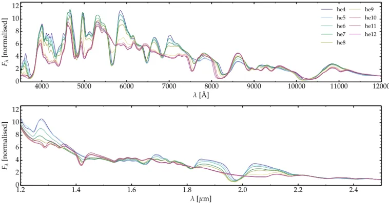
4000 5000 6000 7000 8000 9000 10000 11000 12000 λ[ ˚A] 0 2 4 6 8 10 12 Fλ [normalised] he4 he5 he6 he7 he8 he9 he10 he11 he12 1.2 1.4 1.6 1.8 2.0 2.2 2.4 λ[µm] 0 2 4 6 8 10 12 Fλ [normalised]
Fig. 3.Comparison of the optical (top) and near-infrared (bottom) spectra at bolometric maximum for the He-star explosion models he4–he12.
There is a clear separation between models that show HeIlines (at 5876, 6678, 7065, 10 830, 20 581 Å) and those that do not. Model he9 is an
intermediate case. The presence or absence of HeIlines is easy to see in the optical. HeI10830 Å overlaps with O and Mg lines so a feature is seen
in this spectral region irrespective of the He content. HeI20 581 Å gives a clear signature. We also note that all models have about the same color
at maximum (modulo the strength of lines). For HeIline identifications, see Fig.4.
of two in56Ni mass or explosion energy, or the introduction of
power from a ∼30 ms period magnetar may explain the existence of SNe Ibc with a peak luminosity up to 1042.6erg s−1. With the
exception of a few outliers, this set of models encompasses the whole range of peak luminosities of observed SNe Ibc (Lyman et al. 2016;Prentice et al. 2016). Outliers (i.e., SNe Ibc with a peak luminosity above 1042.6erg s−1) are few and will require
more special circumstances. Because they require an extraordi-nary power source, these outliers may not need to be considered as part of the sample of more standard SNe Ibc.
4. Results: spectral properties
Progenitor models he4 to he12 exhibit a monotonic drop in the mass of the He-rich shell and surface He mass fraction (Fig.1). Model he9 is at the transition between models he4–he8 that have retained a He-rich shell (the shell where He has a 98% mass fraction) and models he10–he12 that have only a low-mass outer shell with some residual He on top of a growing CO core (see Fig.1and Table1). These properties ledYoon(2017) to propose that ejecta models he4–he8 would produce SNe Ib and the rest SNe Ic.
Figure 3 shows the optical and near-infrared spectra for model he4 to he12 at the time of bolometric maximum. This epoch is unambiguously defined and corresponds roughly to the time of spectral classification for many SNe Ibc observed to date. We see that models he4 to he8 have very similar spectral energy distributions, with the obvious presence of HeI5876 Å.
This line is half as strong in model he9, and very weak in mod-els he10–he12. Hence, we see that there is a clear dichotomy for the presence of HeI5876 Å, being present in all models with a
massive He-rich shell (wherein the He mass fraction is essen-tially equal to 1 − Z; models he4 to he8) and being absent in models with a truncated or absent He-rich shell (wherein He is part of a mixture with C, O, Ne, and Mg).
The HeIline strengths are controlled by complex, nonlinear,
nonLTE effects, and strongly influenced by nonthermal pro-cesses (see extensive discussion in Dessart et al. 2012 andLi et al. 2012). Despite this complexity, one can surmise that the progressive drop in the strength of HeI lines is related to the
progressive decline in He abundance (concomitant with the pro-gressive increase in O abundance) in the spectrum formation region (recall that the56Ni abundance profile in velocity space is
similar in models he4–he12 so the mixing is effectively similar in this model set). This region extends from below the photosphere up to large velocities, and is thus not confined to the photosphere. However, the photosphere composition gives a clue as to why the HeIlines become so weak in models he10 to he12. In Table3,
we give the He and O mass fraction at the Rosseland-mean pho-tosphere at the time of maximum. While the He mass fraction stays above ∼0.6 in model he4–he8 (it dominates the composi-tion), it drops below 0.2 in models he10–he12 (it is below 0.2 nearly throughout the ejecta in those models; see Fig. 1). As already discussed in the introduction, the lower He abundance implies that He captures a lower share of the total decay power absorbed by the plasma. This is aggravated by the fact that the ejecta masses increase as we progress from model he4 to he12, while the powering source is kept the same (the56Ni mass is
the same in this model set and equal to 0.08 M ). Since the56Ni
abundance profile is the same in models he4–he12, the chem-ical stratification of our He star models implies that the 56Ni
abundance is greater where He is present in lower-mass He-star models (i.e., model he4 relative to he12). Finally, a lower He
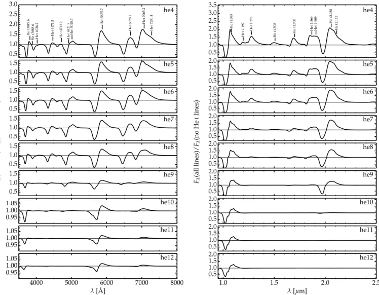
λ[ ˚A] 0.5 1.0 1.5 2.0 2.5 3.0 he4 He I 3819.6 He I 3888.6 He I 4026.2 He I 4471.5 He I 4713.2 He I 4921.9 He I 5015.7 He I 5875.7 He I 6678.1 He I 7065.2 He I 7281.4 λ[ ˚A] 0.5 1.0 1.5 he5 λ[ ˚A] 0.5 1.0 1.5 he6 λ[ ˚A] 0.5 1.0 1.5 he7 λ[ ˚A] 0.5 1.0 1.5 he8 λ[ ˚A] 0.5 1.0 1.5 he9 λ[ ˚A] 0.95 1.00 1.05 he10 λ[ ˚A] 0.95 1.00 1.05 he11 4000 5000 6000 7000 8000 λ[ ˚A] 0.95 1.00 1.05 he12 Fλ (all lines)/ Fλ (no He I lines) λ[µm] 0.5 1.0 1.5 2.0 2.5 3.0 3.5 he4 He I 1.083 He I 1.197 He I 1.278 He I 1.508 He I 1.700 He I 1.869 He I 1.909 He I 2.058 He I 2.112 λ[µm] 0.5 1.0 1.5 2.0 he5 λ[µm] 0.5 1.0 1.5 2.0 he6 λ[µm] 0.5 1.0 1.5 2.0 he7 λ[µm] 0.5 1.0 1.5 2.0 he8 λ[µm] 0.5 1.0 1.5 2.0 he9 λ[µm] 0.5 1.0 1.5 2.0 he10 λ[µm] 0.5 1.0 1.5 2.0 he11 1.0 1.5 2.0 2.5 λ[µm] 0.5 1.0 1.5 2.0 he12 Fλ (all lines)/ Fλ (no He I lines)
Fig. 4.Illustration of the HeIlines in our model sequence he4–he12 at bolometric maximum. The quantity shown is the ratio of the total flux
(i.e., computed by accounting for all bound-bound transitions of all species) with the flux obtained by excluding HeIbound-bound transitions. In
models he4 to he8, HeIlines are not limited to 5876, 6678, and 7065 Å but are instead present throughout the optical up to 7281.4 Å. Their strength
diminishes as we progress from model he4 to he8, and progressively vanish as we progress from model he9 to he12. The ordinate scale is not kept
the same for all panels, to better reveal the strong variation in the strength of HeIlines between models. While HeIoptical lines stand 30 to 60%
above the continuum in models he4–he8, their strength is at the 1% level in models he10–he12 (such weak lines are hard to detect without high S/N).
abundance implies smaller He level populations, which would lower the strength of HeIlines.
Figure3shows that in the near infrared, the HeI1.083 µm
is a poor discriminant for He abundance since it shows a sim-ilar strength in all models he4 to he12 (this stems from the overlap with multiplet lines due to CI, OI, and MgII; Dessart et al. 2015), although the absorption extends to a larger veloc-ity in He-rich models, as expected. In contrast, we find that the HeI2.0581 µm line is an excellent tracer for the presence of a
massive He-rich shell in the progenitor, just like HeI5876 Å in the optical range.
In general, the optical HeIlines that are studied in SNe Ib are
limited to those at 5876, 6678, and 7065 Å. In practice, numerous other HeIlines are present. Figure4shows model spectra for the
sequence he4 to he12 at the time of bolometric maximum (same time as in Fig.3), and more specifically the ratio of the total flux to that obtained by excluding bound-bound transitions associated with HeI. This ratio therefore reflects the contribution (akin to
an equivalent width wherein the ratio is taken between the total
flux and the continuum flux) due to HeIlines. The strength of
HeIlines decreases steadily as we progress through the sequence from ejecta model he4 to ejecta model he12. The maximum HeI
line flux stands ∼50% above the continuum flux in model he4, but drops to only ∼1% above the continuum in model he12 (level at which it is hard to detect).
In the optical, the strongest HeIlines are at 5876 and 7065 Å
(the latter is very broad because it overlaps with HeI7281.4 Å),
followed by HeI6678 Å. However, there are numerous HeIlines
in the blue part of the optical, and specifically at 5016 and 4922 Å (these overlap with FeII lines and may thus be
un-noticed), 4713, 4471, 4026, 3889, and 3820 Å (the last two overlap with CaIIH&K). Other HeI lines in the optical are weaker and thus not discussed here. The HeIlines at 5016 and
4922 Å are at the origin of the difference observed in the 4900 Å region between the mean spectra of SNe Ib and SNe Ic pre-sented by Liu et al. (2016). In the near infrared, besides HeI
lines at 1.083 and 2.058 µm, there are relatively strong HeIlines at 1.278, 1.70, 1.869, 1.909, and 2.112 µm (the latter overlaps
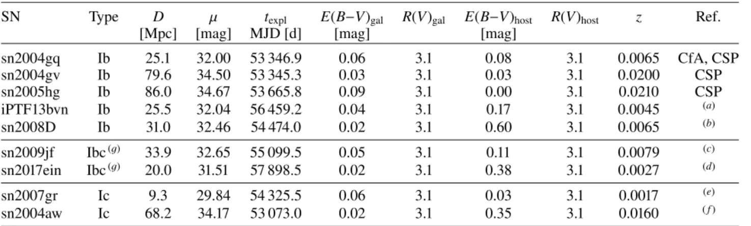
Table 4. Characteristics of our selected sample of Type Ib and Ic SNe.
SN Type D µ texpl E(B−V)gal R(V)gal E(B−V)host R(V)host z Ref.
[Mpc] [mag] MJD [d] [mag] [mag]
sn2004gq Ib 25.1 32.00 53 346.9 0.06 3.1 0.08 3.1 0.0065 CfA, CSP sn2004gv Ib 79.6 34.50 53 345.3 0.03 3.1 0.03 3.1 0.0200 CSP sn2005hg Ib 86.0 34.67 53 665.8 0.09 3.1 0.00 3.1 0.0210 CSP iPTF13bvn Ib 25.5 32.04 56 459.2 0.04 3.1 0.17 3.1 0.0045 (a) sn2008D Ib 31.0 32.46 54 474.0 0.02 3.1 0.60 3.1 0.0065 (b) sn2009jf Ibc(g) 33.9 32.65 55 099.5 0.05 3.1 0.11 3.1 0.0079 (c) sn2017ein Ibc(g) 20.0 31.51 57 898.5 0.02 3.1 0.38 3.1 0.0027 (d) sn2007gr Ic 9.3 29.84 54 325.5 0.06 3.1 0.03 3.1 0.0017 (e) sn2004aw Ic 68.2 34.17 53 073.0 0.02 3.1 0.35 3.1 0.0160 ( f )
Notes. In the following, CfA refers toBianco et al.(2014) and CSP toTaddia et al.(2018).(g)The classification as Ibc arises because of the use of
the intermediate model he9 at the junction between models that are unambiguously associated with SNe Ib (he4–he8) and SNe Ic (he10–he12).
References.(a)Bersten et al.(2014);(b)Modjaz et al.(2009);(c)Valenti et al.(2011);(d)Van Dyk et al.(2018, we take the average of their values for
the distance and the extinction);(e)Hunter et al.(2009);( f )Taubenberger et al.(2006).
with HeI2.0581µm). As visible in Fig.3, there is a clear
sim-ilarity of spectral properties with respect to HeIlines between
models he4 to he8 on the one hand, and model he10 to he12 on the other hand. Model he9 is an intermediate case where the SN classification may be ambiguous.
We see from these simulations that models with a He-rich shell exhibit optical spectra that are nearly exclusively composed of HeIlines (see also early-time models inDessart et al. 2011).
Classifying a SN as Type Ib is trivial in this case. But it also means that whenever there is ambiguity about the classification as Ib or Ic, the progenitor star cannot have a He-rich shell and is most likely poor in He. Here, in models he10–he12, the total mass of He is less than about 0.3 M . With our He-star models,
we see a direct correspondence between the WR classification as type WN or WC, and the SN classification as Type Ib or Ic. 5. Comparison to observations
5.1. Observational data
We selected a small but representative sample of well observed SNe Ib and Ic. One criterion was that both optical and near-infrared photometry was available from premaximum to the nebular phase (in cases where the near-infrared photometry is lacking, we only compare the post-maximum spectrum). Sec-ondly, a good quality spectrum was required around the time soon after maximum. At this epoch, the variations in progeni-tor radius no longer influence the SN radiation, departures from spherical symmetry might be weaker, and the spectrum forma-tion region is extended so that most of the ejecta (in terms of mass rather than velocity since the outermost layers traveling at high speed are optically thin) is probed. Hence, at this epoch, the SN spectrum is primarily sensitive to the composition (He, CNO, intermediate mass elements, iron group elements) and the heating source (which provides the source of radiation, controls the ionization etc). Finally, all data had to be public.
The sample of observed SNe that we selected is presented in Table 4, together with their characteristics (distance, red-dening, redshift) and corresponding references. The sample of SNe Ib includes SNe 2004gq, 2004gv, 2005hg, iPTF13bvn, and SN 2008D. The sample of SNe Ic (or cases that could be consid-ered intermediate between Ib and Ic, although these are markedly
different from the selected SN Ib sample) includes SNe 2009jf, 2017ein, 2007gr, and 2004aw.
Using the observational characteristics of each selected SN, we convert from photometry to flux and build the SN lumi-nosity falling between the B-band and the H-band. In most cases, the values we infer for the peak luminosity is simi-lar to previous simisimi-lar inferences (Lyman et al. 2016; Prentice et al. 2016; Meza & Anderson 2020), although in many cases (including SNe that we do not include in our sample), redden-ing is uncertain (in some cases, literature values seem to be in error). This is particularly relevant because, perhaps because of their association with denser and younger stellar populations, many SNe Ibc are affected by a very large inferred redden-ing, a feature that does not seem so prevalent with SNe II-P. Intriguingly, many SNe Ibc with large inferred peak luminosi-ties (around or above 1042.6erg s−1) also have a large inferred
reddening, so one wonders whether these hard-to-explain lumi-nosities result from an overestimate in the reddening. Finally, the same photometry-to-flux conversion procedure is applied to the photometry of all our models so we can directly compare quasi-bolometric light curves for our sample of observed SNe Ibc and our models (there is thus no concern about the miss-ing flux below and beyond the wavelength range considered). We have tested our procedure on models: taking the flux from CMFGEN, we compute the photometry from U to K, and then proceed back to infer the luminosity falling between U and K. This gives the same result at the percent level as that obtained by computing this luminosity directly from the original CMFGEN spectrum.
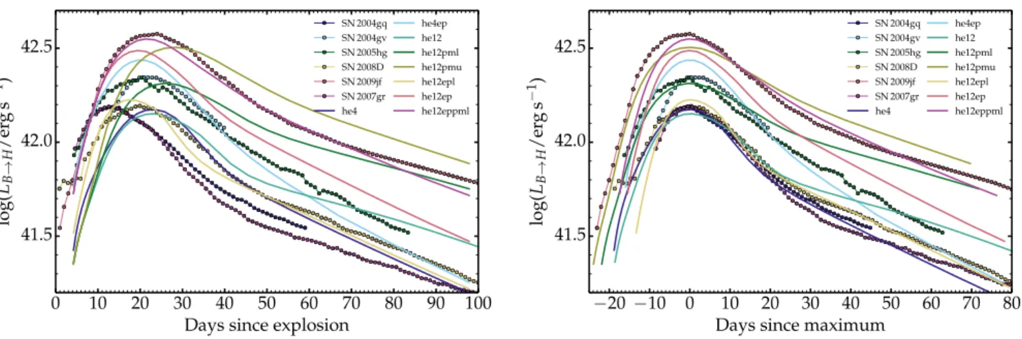
5.2. Light curve comparisons
Figure5compares the B to H luminosity evolution for our sam-ple of SNe Ib and Ic (we only include the observed SNe that have photometry covering B to H) with a limited set of our models. As evident from Fig.2, the ejecta mass has a weak influence on our model light curves during the photospheric phase because by design we adopted a fixed value of Ekin/Mej for the model
sequence he4 to he12. The selection of models shown in Fig.5is thus limited to he4, he4ep, he12, he12epl, he12ep (he4 and he12 on the hand, and he4ep and he12ep appear similar; he12epl is the counterpart to he12ep but with the same56Ni mass as he12),
0 10 20 30 40 50 60 70 80 90 100 Days since explosion
41.5 42.0 42.5 log( LB→ H /er g s − 1) SN 2004gq SN 2004gv SN 2005hg SN 2008D SN 2009jf SN 2007gr he4 he4ep he12 he12pml he12pmu he12epl he12ep he12eppml −20−10 0 10 20 30 40 50 60 70 80
Days since maximum 41.5 42.0 42.5 log( LB→ H /er g s − 1) SN 2004gq SN 2004gv SN 2005hg SN 2008D SN 2009jf SN 2007gr he4 he4ep he12 he12pml he12pmu he12epl he12ep he12eppml
Fig. 5.Evolution of the luminosity falling within the B and H bandpasses for a sample of SNe Ibc and a representative sample of models taken from this study. The time origin is the time of explosion (left) or the time of maximum luminosity (right).
and then some variants of he12 with magnetar power (he12pml, he12pmu, he12eppml) – see Table2for details.
In the left panel of Fig.5, the light curves are shown with respect to the time of explosion (or rather the inferred time of explosion for the observations). One sees that the models encom-pass the range of peak luminosities between (relatively) fainter events like SN 2008D and brighter events like SN 2009jf. None of the models fit perfectly but it is clear that by invoking vari-ous combinations of the present range of ejecta masses, kinetic energies, 56Ni mass, and a moderate power from the compact
remnant, one can cover the parameter space occupied by the majority of SNe Ibc observations. The models show a wide range of decline rates at nebular times: modulations in γ-ray escape can lead to a fast decline, while at the opposite extreme, introduction of magnetar (or fallback-accretion) power leads to a slower fad-ing at late times (as would also occur in the case of full trappfad-ing of γ-rays from56Co decay).
For a number of models, there is a discrepancy in the rise time. Most of our models peak around 21 d after explosion (see Table2; one exception is model he12epl, characterized by a large Ekinof 4.8 × 1051erg but a modest56Ni mass of 0.08 M ) while
numerous observed SNe Ibc have an inferred time of explo-sion between about 10 and 15 d. If real, this short rise time requires models with a larger Ekin/Mej (as in model he12epl).
Since the explosion energy applied in our models (for exam-ple he4ep, he12epl, or he12ep) is already large, in tension with what the explosion mechanism can allow (seeErtl et al. 2020), one way to explain such short rise times is to invoke smaller ejecta masses, probably in the range 0.5–1 M . In our sample,
this applies especially to the Type Ib SN 2004gq (which could arise from a low-mass He giant; see, for example,Eldridge et al. 2015; Dessart et al. 2018) and to the Type Ic SN SN2007gr (which could arise from Case BB mass transfer in a tight binary;
Dewi et al. 2002;Dewi & Pols 2003; Tauris et al. 2015). The latter scenario was proposed to explain the observations of the fast rising and fast declining Type Ic SN 1994I (Nomoto et al. 1994).
When plotting the same B to H luminosity evolution but now with respect to the time of maximum (right panel of Fig.5), the agreement between observations and models is much improved. The light curves of SNe 2004gq (Type Ib) and 2007gr (Type Ic), which nearly overlap, are well matched by model he4 and he12, confirming the proximity of SNe Ib and Ic light curves despite their distinct SN type (Drout et al. 2011). This suggests that the
main source of discrepancy here is the ejecta mass (for the fast rising SNe) while SNe Ibc with slightly higher peak luminosi-ties may be explained by a weak power contribution from the compact remnant.
The existence of even more luminous SNe Ibc presents the same theoretical challenge that pertains to the existence of GRB/SNe Ic, SNe Ic-BL, or super-luminous SNe Ic. Luminous SNe Ibc may be considered transition objects between standard SNe Ibc and SNe Ic-BL or GRB/SNe. The theory explaining the latter would apply at a more moderate level in those transition objects.
In Prentice et al. (2016), SNe Ibc (excluding GRB/SNe, SNe Ic-BL, and SNe IIb) with a peak luminosity greater than 1042.6erg s−1are SN 2007C, SN 2007uy, SN 2009er, SN 2011bm,
PTF 11rka, and PTF 12gzk. Let us inspect these peak lumi-nosities in more detail. For SN 2007C, Prentice et al. (2016) use a total reddening E(B−V) of 0.77 mag and a distance of 26.9 Mpc. However,Meza & Anderson (2020) use a total red-dening that is much lower, with E(B−V) of 0.47 mag. This implies a 0.37 dex lower peak luminosity, bringing SN 2007C much below 1042.6erg s−1. For SN 2007uy, the inferred
redden-ing is large with E(B−V) of 0.65 mag, yieldredden-ing a peak luminosity of 1042.67erg s−1 (Prentice et al. 2016) or 1042.58erg s−1 (Meza & Anderson 2020). However, comparing the maximum light spectrum of SN 2007uy to that of SN 2008D (which has a similar inferred reddening), one sees that SN 2007uy is much bluer, meaning it is likely not as reddened. Hence, just like for SN 2007C, the reddening of 0.65 mag used for SN 2007uy is likely overestimated and therefore the peak luminosity of that SN is probably smaller, bringing it below 1042.6erg s−1. SN 2009er is
classified as a Type Ib-pec byBianco et al.(2014) so not a stan-dard SN Ib nor Ic. SN 2011bm and PTF 11rka possess very broad light curves and large sustained luminosities at nebular times. Perhaps these are intermediate events requiring a magnetar (or whatever extra power source), and standing between standard SNe Ibc and objects like SNe 2005bf (Tominaga et al. 2005;
Folatelli et al. 2006;Maeda et al. 2007) and SLSNe Ic (Pastorello et al. 2010;Quimby et al. 2011). Finally, PTF 12gzk shares sim-ilar properties to SNe Ic-BL and is thus not a standard SN Ic (Ben-Ami et al. 2012). The evolutionary paths and metallicities leading to GRB/SNe and SLSNe Ic are distinct from those rele-vant to the majority of SNe Ibc (Aguilera-Dena et al. 2018). We thus see that an overestimate in the reddening is in part respon-sible for the large inferred peak luminosities (the error applies to
the whole light curve) of several SNe Ibc that have so far been considered outliers in the community.
So, from this exploration, we see that all SNe Ibc hav-ing a peak luminosity above 1042.6erg s−1 are either peculiar
events, extraordinary events like SNe Ic-BL or GRB/SNe, or were given an overestimated reddening. We can draw a paral-lel with SNe II. What would be the distribution of SNe II peak luminosities (or luminosities at 10 d after explosion or discovery, since most SNe II do no have a clear peak in their bolometric light curve) if we included all H-rich events? We would find low luminosity events (the faint SNe II-P), standard-luminosity events (SNe II-P and SNe-pec, powered by shock deposited energy prior to shock breakout, and56Ni decay power), and then
very luminous events (all SNe IIn, in which the power arises from interaction with CSM). Explaining this whole range with a56Ni-power model combined with the standard neutrino-driven
mechanism would lead to an inconsistency. This inconsistency may arise because high luminosity events are not powered by
56Ni. The same applies to the SN Ibc sample, for which one
finds that the 56Ni-power model combined with the standard
neutrino-driven mechanism cannot explain the high-luminosity end. These brighter events probably owe their luminosity to a distinct power source.
It thus seems that the grid of models we present here, based on moderate explosion energies, a range of56Ni masses between
0.08 and 0.16 M , or boosted by a slowly rotating magnetar can
reproduce the energetics of nearly all SNe Ibc light curves. There is no “extreme” physics involved here. SNe Ibc that are more luminous at maximum and sometimes later require extra power from the compact remnant. It thus seems plausible that SNe Ibc arise from a standard core-collapse explosion mechanism, at best aided by a modest energy injection from the compact remnant (Ertl et al. 2020). Such a modest extra power may also be present in Type II SNe but difficult to quantify because their ejecta are optically thick for much longer than in SNe Ibc.
5.3. Spectral comparisons early after maximum light
An advantage of our modeling with CMFGEN is the computation of the time evolving spectral energy distribution, from which one can extract the bolometric light curve, photometric light curve in any bandpass, as well as the spectral evolution in any wave-length region between 100 Å and 100 µm. In other words, the same numerical code yields the information on the photometric and spectroscopic evolution of a given model. Only few codes in the community use this approach, but with a different treatment of nonLTE processes and typically not applied to the modeling of SNe Ibc (SEDONA,Kasen et al. 2006; ARTIS,Sim 2007;Kromer & Sim 2009; JEKILL,Ergon et al. 2018). In contrast, SN studies generally use distinct codes with distinct physics to compute the photometric and spectroscopic evolution, so that physical con-sistency is not guaranteed in those works. We have presented numerous studies of SNe Ibc in the past, and showed their full bolometric, multi-band photometric, color, and spectral evolu-tion from early to late times (Dessart et al. 2011,2012, 2015,
2016,2017). Here, we focus on the spectral properties around the time of maximum.
Figure6presents a comparison of optical spectra of SNe Ib and Ic with a selection of our models. The observed spectra are first corrected for redshift and reddening, and then normalized to the model spectra at a wavelength between 6000 and 7000 Å. This normalization is done to ease the comparison. In practice, the offset in absolute V-band magnitude between observations
and models at the corresponding epoch is shown in the label at right (a negative value means that the observations are brighter than the model). The label also gives the SN name, the model name, and the time elapsed since V-band maximum for both. The color coding is used to group together the SNe Ib (models in red), the intermediate cases between SNe Ib and Ic (models in yellow), and the SNe Ic (models in green). Here, the grouping by SN type is not meant to reflect any specific equivalent-width estimate for the strength of putative HeIlines. Instead, we search for a global
compatibility between observed and model spectral properties. Our goal is to check whether our grid of stellar evolution and explosion models mirrors the diversity of observed SNe Ib and Ic.
The SNe Ib that show unambiguously HeI lines are well
fitted with models he4 and he6 (models he4 to he8 fare well due to their similar spectral properties – see Figs.3and 4). As discussed in Sect. 4, these lines are not limited to HeI5876, 6678, and 7065 Å. We also identify HeIlines at 4471, 4922 and
5016 Å. Hence, in what we could call “genuine” SNe Ib, most optical lines are due to HeI. Other lines are due to CaIIH&K, FeII5169 Å, OI7774 Å and the CaIInear-infrared triplet. The
spectral properties are very similar for this sample of SNe Ib at early times post V-band maximum. One discrepancy is the much larger line width in SN 2004gq compared to model he4 but this stems primarily from the very short rise time of about 13 d in SN 2004gq, thus 10 d less than in model he4. We also find that SN 2005hg can be well fitted with model he6, with an offset of −0.35 mag in V (the SN is a little brighter than the model at the post-maximum epoch). The good match to the optical color suggests that our adopted total reddening of E(B−V) = 0.09 mag is suitable. The choice of E(B−V) = 0.685 mag byLyman et al.
(2016) is an error and it is the origin of their inference of a large peak magnitude of −19.2 mag and the erroneous status of prominent outlier for SN 2005hg in the type Ib SN class. Instead, SN 2005hg appears as a standard Type Ib SN.
For SNe 2009jf and 2017ein, we used model he9 and he9pml – progenitor model he9 is intermediate between Ib and Ic (see Sect. 2.1). Overall, the models reproduce most of the features although the model he9pml is too faint compared to SN 2009jf. Matching the line widths is difficult since some are overes-timated while others are underesoveres-timated by the model. This may be caused by the adopted mixing (Dessart et al. 2012), but may also be a signature of asphericity, for which we have unambiguous evidence in stripped-envelope SNe (Rest et al. 2011).
For SNe 2007gr and 2004aw, we use models that show no HeIlines (see Fig.4). Model he10 fits well SN 2007gr (despite
the offset in rise time to maximum) while the comparison to SN 2004aw required the higher energy model he12ep, in agree-ment with previous studies (Taubenberger et al. 2006;Mazzali et al. 2017). We also tried models with magnetar power. Model he12pml is a little too faint and underestimates line widths. Model he12pmu matches the brightness but is too blue and also underestimates line widths.
As far as we know, this is the first time that a single set of progenitor models, computed consistently from stellar evo-lution and exploded in a standard fashion (here using a thermal bomb to yield energies commensurate with theoretical expec-tations), reproduces the dichotomy between SNe Ib and SNe Ic spectral properties, as well as the photometric properties of a rep-resentative SN Ibc sample. The discrepancy in rise time between our models and some observations suggest lower ejecta masses, likely produced by binary mass exchange after He-core burning (as would be produced by case BB mass transfer).
4000
5000
6000
7000
8000
9000
10000
11000
Rest Wavelength [ ˚A]
F
λ+
Const.
he4/04gq/+16.1d/ 0.17 he4/04gv/+11.9d/-0.28 he4/13bvn/+8.5d/-0.18 he6/05hg/+12.0d/-0.35 he6/08D/+14.5d/ 0.11 he9pml/09jf/+9.6d/-0.61 he9/17ein/+12.8d/ 0.15 he10/07gr/+10.5d/ 0.00 he12ep/04aw/+10.9d/-0.07 Model/SN/Age/∆MVFig. 6.Comparison of observed optical spectra (corrected for redshift and reddening; see Table4) for a sample of SNe Ib, and Ic with a selection of models from this study. Colors red, yellow, and green correspond to type Ib, Ibc, and Ic SN models.
6. Discussion
The simulations we present in this paper show a degeneracy in light curve and spectral properties for ejecta with a compara-ble Ekin/Mej. The representative ejecta expansion rate being the
same for ejecta with the same Ekin/Mej, the spectral line widths
are also comparable. It is therefore challenging to separately con-strain Ekinand Mej. There is no unique ejecta model to a given
light curve and spectrum at maximum. Another way of stating this is that for any given model, one can find a counterpart at
lower or higher Ekin (or Mej) that will exhibit the same light
curve and the same spectrum at maximum, and potentially the same spectral evolution at all times1. In practice, this may be complicated further by the presence of a chemical stratification
1 A similar degeneracy was observed in the grid of SN Ic
simu-lations presented in Dessart et al. (2017) and Dessart (2015). For
example, one ejecta model with Ekin=4 × 1051erg and Mej=10 M
yielded the same photometric and spectroscopic properties from 3 to
200 d after explosion as a model counterpart with Ekin=1.1 × 1051erg