HAL Id: hal-00967124
https://hal.inria.fr/hal-00967124
Submitted on 28 Mar 2014
HAL is a multi-disciplinary open access archive for the deposit and dissemination of sci-entific research documents, whether they are pub-lished or not. The documents may come from teaching and research institutions in France or
L’archive ouverte pluridisciplinaire HAL, est destinée au dépôt et à la diffusion de documents scientifiques de niveau recherche, publiés ou non, émanant des établissements d’enseignement et de recherche français ou étrangers, des laboratoires
Verification of the Functional Behavior of a
Floating-Point Program: an Industrial Case Study
Claude Marché
To cite this version:
Claude Marché. Verification of the Functional Behavior of a Floating-Point Program: an In-dustrial Case Study. Science of Computer Programming, Elsevier, 2014, 93 (3), pp.279-296. �10.1016/j.scico.2014.04.003�. �hal-00967124�
Verification of the Functional Behavior of a
Floating-Point Program: an Industrial Case Study
Claude Marchéa,b
aInria Saclay - Île-de-France, Palaiseau, F-91120 bLRI, Univ. Paris-Sud, CNRS, Orsay, F-91405
Abstract
We report on a case study that was conducted as part of an industrial research project on static analysis of critical C code. The example program considered in this paper is an excerpt of an industrial code, only slightly modified for confiden-tiality reasons, involving floating-point computations. The objective was to estab-lish a property on the functional behavior of this code, taking into account round-ing errors made durround-ing computations. The property is formalized usround-ing ACSL, the behavioral specification language available inside the Frama-C environment, and it is verified by automated theorem proving.
Keywords: Deductive Program Verification, Automated Theorem Proving, Floating-Point Computations, Quaternions
1. Introduction
The objective of the U3CAT project1was to design various kind of static
ana-lyses of C source code, to implement them inside the Frama-C environment [1], and to experiment them on critical industrial C programs. A part of this project was focused on the verification of programs involving floating-point computa-tions. Several case studies of this particular kind were proposed by industrial partners of the project, and were analyzed using techniques based on abstract in-terpretation and on deductive verification.
1This work was partly funded by the U3CAT project (ANR-08-SEGI-021,
http://frama-c. com/u3cat/) of the French national research organization (ANR), and the Hisseo project, funded by Digiteo (http://hisseo.saclay.inria.fr/)
This paper reports on one such case study. A functional property of its behav-ior is formalized using ACSL—the behavbehav-ioral specification language of Frama-C— and proved using a combination of automated theorem provers. These are either fully automatic ones: SMT (Satisfiability Modulo Theories) solvers Alt-Ergo [2, 3], CVC3 [4] and Z3 [5], the solver Gappa [6] for real arithmetic; or the interactive proof assistant Coq [7].
We first present in Section 2 the case study itself and the functional prop-erty that should be validated. We discuss there why we believe this case study is interesting to publish. In Section 3 we describe the basics of the verification environment in which we verified the program: Frama-C, the ACSL specification language [8] including its specific features about floating-point computations, and the Jessie/Why plug-in [9,10,11] for deductive verification in Frama-C. We em-phasize an important point of the methodology we followed: in a first step, one should specify the program, and prove it, using an idealized model of execution, where no rounding errors occur, that is where computations are assumed to be made in infinite precision. This is the mode we use to perform a preliminary anal-ysis of the case study in Section 4. Only in a second step one should adapt the specifications, and the proof, to take into account rounding errors in floating-point computations: this is done for our case study in Section5.
2. Presentation of the Case Study
The case study was provided by the company Sagem Défense et Sécurité (http://www.sagem-ds.com/), which is part of the larger group Safran. It is spe-cialized in high-technology, and holds leadership positions in optronics, avionics, electronics and critical software for both civil and military markets. Sagem is the first company in Europe and third worldwide for inertial navigation systems used in air, land and naval applications.
The case study is an excerpt of a code related to inertial navigation, that deals with rotations in the three-dimensional space. A standard representation of such rotations makes use of the mathematical notion of quaternions [12]. To perform the verification of that case study, there is indeed no need to understand why or how this representation works. We summarized below only the basic notions about quaternions that are needed for our purpose.
2.1. Quaternions in a Nutshell
Basically, the set of quaternions H can be identified with the four-dimensional vector space R4
with the operations of addition and multiplication by a scalar. A common notation is made by choosing some basis denoted as(1, i, j, k), so that every quaternion q is uniquely written as a linear combinationq1+ q2i + q3j + q4k. Using this basis, the multiplication of two quaternions can be defined thanks to the identities
i2 = j2 = k2 = −1 ij = k jk = i ki = j ji = −k kj = −i ik = −j leading to the formula
(q1+ q2i + q3j + q4k) × (p1+ p2i + p3j + p4k) = q1p1− q2p2− q3p3 − q4p4+
(q1p2+ q2p1+ q3p4− q4p3)i+ (q1p3− q2p4+ q3p1+ q4p2)j+ (q1p4+ q2p3− q3p2 + q4p1)k It is worth to remind that multiplication is not commutative.
The norm of a quaternion is also defined, as ||q|| = q q2 1 + q 2 2 + q 2 3 + q 2 4
Among other properties, an important property is that the norm of a product is equal to the product of the norms. Quaternions of norm 1 are of particular interest for representing rotations.
2.2. The Source Code
The source code that was given to analyze mainly amounts to repeatedly mul-tiplying a quaternion by other quaternions that come from some external sources of measure. The simplified source code is given on Figure 1, where the external source of quaternion is abstracted by the C function random_unit_quat return-ing an arbitrary quaternion. In C, a quaternion is represented by an array of four double-precision floating-point numbers (typedouble). We remind that the preci-sion of type doubleis 53 binary digits, meaning that the relative precision of the representation of real numbers is approximately10−16.
The arbitrary quaternions returned by function random_unit_quat are in-tended to be of norm 1, so the repeated multiplication should in principle remain of norm 1 over time. However, due to the imprecision of the floating-point repre-sentation, this property is not valid. First, the norm of those arbitrary quaternions
typedef double quat[4];
/// copy of a quaternion
void Quat_copy(const quat src,quat dst) { dst[0] = src[0]; dst[1] = src[1]; dst[2] = src[2]; dst[3] = src[3]; } /// multiplication of quaternions
void Quat_prod(const quat q1, const quat q2, quat q) {
q[0] = q1[0]*q2[0] - q1[1]*q2[1] - q1[2]*q2[2] - q1[3]*q2[3]; q[1] = q1[0]*q2[1] + q1[1]*q2[0] + q1[2]*q2[3] - q1[3]*q2[2]; q[2] = q1[0]*q2[2] - q1[1]*q2[3] + q1[2]*q2[0] + q1[3]*q2[1]; q[3] = q1[0]*q2[3] + q1[1]*q2[2] - q1[2]*q2[1] + q1[3]*q2[0]; }
/// returns a random quaternion of norm 1
void random_unit_quat(quat q);
/// repeated multiplication of quaternions of norm 1
int test1(void) {
quat current, next, incr; random_unit_quat(current); while (1) { random_unit_quat(incr); Quat_prod(current,incr,next); Quat_copy(next,current); } return 0; }
cannot be exactly 1, only close to 1 up to a small amount. Second, due to addi-tional imprecisions of the computation of multiplication, the norm of the iterated multiplication is going to slowly drift over time. In a critical application, this drift may be dangerous2, so the original code “re-normalizes” the quaternioncurrent,
in the sense that its components are divided by its norm, so as the norm hopefully remains close to 1. Hence for our given code without re-normalization, one can only try to establish that the norm remains close to 1 for a limited time.
2.3. The Property to Establish
One can express the drift of the norm of current as a function of the num-ber of iterations. If there is an acceptable upper bound on the drift, then the re-normalization may safely be dropped. The aim was to find such a bound and to prove its correctness.
Looking at the code, one (reasonably experienced in floating-point computa-tions) observes that the rounding error on the norm of a product is bounded by some constant, so the property that we can think of is of the form
(1 − ε)n ≤ ||current|| ≤ (1 + ε)n
wheren is the number of iterations, and ε is some constant to be determined, of course as small as possible.
In the remainder of the paper, we will discuss only the right part of that prop-erty:
||current|| ≤ (1 + ε)n the left part being treated analogously.
2.4. Significance of the Case Study
Although the program is very small, this case study should be considered as “industrial” for two main reasons. First it is provided by a true industrial company, from a true program that they developed. Second, the property that we have to address is a real issue that they want to solve.
The case study is significant from both an industrial and an academic point of view.
2In fact, this kind of loss of precision over time due to iterated rounding errors is a typical issue in critical C code: the famous bug of the Patriot missile battery (See http://www.ima. umn.edu/~arnold/455.f96/disasters.html) was of this kind, an internal clock being iteratively incremented by step of 0.1seconds, although unfortunately 0.1is not exactly representable neither as a fixed-point nor as a floating-point number [13].
• For an industrial, the property to address is a complicated one. The only ap-proach that was possible for our industrial partner is to perform iteration of product of randomly generated quaternions and observe the drift over time. The results suggest that the norm remains close to 1 for a significant time, but random testing does not provide a strong guarantee, and an analysis of the worst case is required.
Knowing a bound in the worst case may allow the author of the code to get rid of the cost of re-normalization that it is done currently, which may permit to iterate the capture of motion at a higher rate. It is thus desirable to know whether there exists methods and tools in academia with which such a property can be addressed.
• For academic researchers, it is good to have such an example of a property that is needed in “real life”. This kind of property, bounding the accumu-lated rounding error over time, is clearly not widely studied until now. It is a good thing to publicize such concrete examples, since industrial examples are usually not easily accessible to academia.
Making such an example public naturally provides interesting material for tool developers. They should be interested in demonstrating that their fa-vorite approach is able to cope with such a problem. Also, several authors willing to provide their own solutions to the same problem generates a con-structive kind of competition, in the same spirit as verification competitions organized recently [14,15].
For us, the goal is to show how we addressed the problem with the Frama-C/Jessie tool suite, what kind of strong or weak features we identified, and then encourage people to use the tool suite if they have similar problems to solve, in a better informed way.
3. Basics of the Verification Environment
To conduct this case study, we used the Jessie plug-in [9, 10] of Frama-C. The analysis method performed by this plug-in is of the kind of deductive verifi-cation. It amounts to formalize the expected properties using a formal specifica-tion language, then to generate verificaspecifica-tion condispecifica-tions: logic formulas that should be proved valid, so as to establish that the code respects the given specification. Those formulas are typically discharged using automated theorem provers.
Significant progress was made in recent years on the development of verifi-cation systems based on deductive verifiverifi-cation, in particular those dedicated to mainstream programming languages. Several mature environments exist nowa-days: systems like ESC-Java2 [16], Mobius PVE (http://kindsoftware.com/ products/opensource/Mobius/), Jahob [17] can deal with Java code typically annotated with JML [18]; VCC [19] deals with C code, Spec# [20] deals with C# programs, Spark [21] with Ada programs, etc. Frama-C also belongs to this collection: it is an environment for static analysis of C code. Its architecture is extensible: it is built around a kernel providing C files parsing and typing, and static analyzers can be plugged-in under the form of dynamically loaded libraries. Among others, two Frama-C plug-ins are specialized in deductive verification: WP and Jessie. Frama-C kernel implements the specification language ACSL [8]. As far as we know, none of the systems above provide a faithful support for floating-point computations. Only the Jessie plug-in of Frama-C has such a fea-ture [22], which was designed during the U3CAT project. This support is based in part on an extension of the ACSL specification language.
3.1. An Illustrative Example
We present the basics of the use of Frama-C/Jessie, and the main components we need from the ACSL language. The process for verifying a C source code with respect to a functional requirement is first to annotate the source with ACSL clauses formalizing the requirement, and run Frama-C and the Jessie plug-in on the annotated code. Jessie translates the annotated code into the Why3 [23, 24] intermediate language, that includes a verification condition generator. These con-ditions are then visualized in a graphical interface that allows the user to run ex-ternal provers on them. The programs of this paper were analyzed with Frama-C version Oxygen, Jessie version 2.32, and Why3 version 0.81.
To illustrate this process, consider the following example originally proposed by Ayad [22]. This is a small C function that aims at computing an approximation of the exponential function on the domain[−1; 1]
double my_exp(double x) {
return 0.9890365552 + 1.130258690 * x + 0.5540440796 * x * x; }
the formula used in this code implements a so-called Remez polynomial approx-imation of degree 2. A typical requirement is naturally to state a bound on the difference between the result computed by this function on an argumentx and the true real value exp(x). Such a requirement must include the assumption that x
is in the interval [−1; 1]. Using the ACSL language, such a requirement is for-malized by stating a contract on the C function, which is basically made of a precondition and a post-condition. Such a contract is inserted in the C code inside the special form of comments/*@ ... @*/. On this example we can write
1 /*@ requires \abs(x) <= 1.0;
2 @ ensures \abs(\result - \exp(x)) <= 0x1p-4; 3 @*/
4 double my_exp(double x) { 5 ...
Therequires clause on line 1 introduces the precondition, using\abswhich is a built-in symbol in ACSL and denotes the absolute value. Theensures clause on line 2 introduces the post-condition. It states that ifr is the result of the function call, then |r − exp(x)| ≤ 1
16 (notations of the form0xhh.hhpdd are hexadeci-mal FP literals, where h are hexadecimal digits and dd is in decimal, and denote numberhh.hh × 2dd, hence0x1p-4is2−4). The symbol
\expis also built-in, and
denotes the true mathematical exponential function. We emphasize a very impor-tant design choice in the design of ACSL extensions to support floating-point pro-grams: there is no floating-point arithmetic in the annotations. In specifications, the operators+, −, ∗, / denote operations on mathematical real numbers. Thus, neither rounding nor overflow can occur in logic annotations. Moreover, in anno-tations any floating-point program variable, or more generally any C left-value3
of typefloatordouble, denotes the real number it represents. The post-condition of our illustrative example should read precisely as: take the real numberr rep-resented by the result of this function, and the real numberx represented by the argument x, then it is guaranteed that the formula|r − exp(x)| ≤ 1
16 holds in the true mathematical sense, without the shortcomings of programming languages.
Given such an annotated program, the tool chain Jessie/Why3 must interpret both the annotations and the code. The Jessie plug-in interprets computations in the code faithfully with respect to the IEEE-754 [25] standard for floating-point arithmetic4, whereas the formulas in annotations are interpreted in the first-order
logic of real numbers. This has an important impact on the generated verification 3That is, any expression that may appear in the left part of an assignment.
4We assume in this paper that the compiler and the underlying architecture respect this stan-dard. See D. Monniaux survey [26] on the compilers and architecture issues related to floating-point computation. There are also proposals for architecture-dependent interpretations in the con-text of Frama-C [27,28,29,30].
conditions: those formulas include real arithmetic, and also an explicit rounding functionrnd : R → R such that rnd(x) returns the floating-point number closest tox. Indeed if we run the tool chain on our annotated code, none of the theorem provers is able to discharge the generated condition. To proceed with the proof, we must insert an intermediate assertion in the code, to state an intermediate property. In our example this is done as follows.
double my_exp(double x) { /*@ assert \abs(0.9890365552 + 1.130258690*x + @ 0.5540440796*x*x - \exp(x)) <= 0x0.FFFFp-4; @*/ return 0.9890365552 + 1.130258690 * x + 0.5540440796 * x * x; }
The assertion seems just a paraphrase of the code, however since annotations are interpreted as real number computations, it is quite different: it states that the expression|0.9890365552+1.130258690x+0.5540440796x2
−exp(x)| evaluated as a real number, hence without any rounding, is not greater than 1
16(1 − 2 −16). This intermediate assertion naturally specifies the method error, induced by the mathematical difference between the exponential function and the approximating polynomial, whereas the post-condition takes into account both the method error and the rounding errors added by floating-point computations. This explains why we need a bound on the method error slightly lower than 161: we want the sum of the method error and the rounding error not to exceed 161 .
Indeed, since the method error is a purely mathematical property, it is handy to turn it into a general lemma. In ACSL, this is done as a global annotation as follows.
/*@ lemma method_error: \forall real r; \abs(r) <= 1.0 ==> @ \abs(0.9890365552 + 1.130258690*r +
@ 0.5540440796*r*r - \exp(r)) <= 0x0.FFFFp-4; @*/
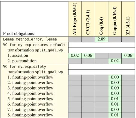
With this additional lemma and the assertion, the generated verifications can be proved automatically, by using a combination of provers. The results are shown5 on Figure2.
The assertion in the code is easily proved by SMT solvers Alt-Ergo, CVC3 and Z3, as a direct consequence of the global lemma. Other verification
Proof obligations Alt-Er go (0.95.1) CVC3 (2.4.1) Coq (8.4) Gappa (0.16.4) Z3 (4.3.1)
Lemma method_error, lemma 2.89 VC for my_exp_ensures_default transformationsplit_goal_wp 1. assertion 0.02 0.06 0.06 2. postcondition 0.02 VC for my_exp_safety transformationsplit_goal_wp 1. floating-point overflow 0.00 2. floating-point overflow 0.00 3. floating-point overflow 0.00 4. floating-point overflow 0.00 5. floating-point overflow 0.01 6. floating-point overflow 0.01 7. floating-point overflow 0.00 8. floating-point overflow 0.01
Figure 2: Proof results of the illustrative example
ditions are the post-condition, but also a series of automatically inserted condi-tions to guarantee the absence of overflow in the code. All these formulas in-volve the rounding operator rnd, that is not known by provers except one par-ticular solver available as a back-end: Gappa [31]. It is a constraint solver for formulas mixing real numbers and rounding operations. Using interval arith-metic, it is able to find upper bounds on arithmetic expressions. Last but not least, the lemma itself should be proved. Since it involves the exponential op-erator, there is no fully automated prover (in Frama-C) that can handle it. In-deed such a prover exists: Metitarski [32], but it is not available from Frama-C/Jessie. Thus we must switch to an interactive proof assistant, here we use Coq [7]. Fortunately, in Coq there is a special tactic for proving bound prop-erties on real expressions involving transcendental functions: the intervaltactic (https://www.lri.fr/~melquion/soft/coq-interval/). Proofs are generated using approximations, again based on interval arithmetic [31]. The Coq proof script for our lemma is just 2 lines long:
intros r h1.
3.2. General remarks on the approach
The case studies we conducted in the past allowed us to learn a few lessons on the good practice when specifying and proving floating-point programs.
• Before trying to deal with a program with a faithful IEEE-754 interpretation of floating-point computations, it is better to specify and prove it using an idealized interpretation were computations are made in real numbers, that is as if computations were done with infinite precision. Such a mode is available in the Jessie plug-in as a global option. This preliminary step is useful to identify the mathematical properties that are assumed by the code. The use of the faithful IEEE mode should be made only when this preliminary version is fully proved.
• To prove all the verification conditions, the user must acquire a good under-standing of the respective abilities of back-end provers, in particular identi-fying the ones that should be proved by Gappa: those are the formulas that state a bound on rounding errors.
• Related to rounding errors, determining the appropriate bound is an issue by itself. For example, how did we determine the bound 161 in our illustrative example? This can be also done by Gappa: the bound can be first given as a unknown parameter, and Gappa being a solver, it is able to give the best bound it can deduce.
4. Verification using Infinite Precision Model
We start by analyzing the code of our case study using the infinite precision model, so double now stands for real, and the basic operations are computed in infinite precision. We first detail how the code is annotated in order to formally specify the properties to prove, before proceeding with the proofs.
4.1. Specifications
For the specifications we need to introduce new definitions, under the form of logic function symbols, as is permitted by the ACSL language. Since quaternions appearing in the code are pointers to blocks of four double-precision numbers, our function symbols will take such pointers as arguments. To ease reading, we introduce a type abbreviation for that.
1 /*@ predicate quat_eq{L1,L2}(quat_ptr q1, quat_ptr q2) =
2 @ \at(q1[0],L1) == \at(q2[0],L2) && \at(q1[1],L1) == \at(q2[1],L2) 3 @ && \at(q1[2],L1) == \at(q2[2],L2) && \at(q1[3],L1) == \at(q2[3],L2); 4 @*/ 5 6 /*@ requires \valid(src+(0..3)); 7 @ requires \valid(dst+(0..3)); 8 @ assigns dst[0..3]; 9 @ ensures quat_eq{Here,Old}(dst,src); 10 @*/
11 void Quat_copy(const quat src,quat dst);
Figure 3: Specification ofQuat_copy
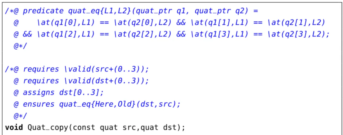
4.1.1. The copy function
To specify the behavior of the copy function, we need to define the notion of equality of two quaternions. The definition of such an equality predicate, and the contract given to the copy function, are shown on Figure3.
The two parameters{L1,L2}(line 1) in the definition of thequat_eqpredicate
are labels denoting memory states [8]. Indeed the definition of that predicate de-pends on the content of the memory pointed to by q1 and q2, hence we make use of the ACSL construct \at(e, L)denoting the value of expression ein the state denoted by label L. Thus, the proposition quat_eq{L1,L2}(q1,q2) reads as “the quaternion pointed by q1 in memory state L1is the same as the quaternion pointed by q2in memory state L2”. It is naturally defined by the equality
com-ponent per comcom-ponent. An alternative definition one may imagine is to define quat_eq taking parameters of type quatand then getting rid of labels. However this would not work as expected: in C, even if a function parameter is declared as typedouble[4], it is interpreted exactly the same as it wasdouble*, and is passed by reference. Thus the type ofsrcanddstis indeeddouble*.
The contract for Quat_copy contains first two preconditions (on lines 6-7)
meaning that the pointer argumentssrcanddstshould point to valid blocks of size 4 in memory. The assigns clause (on line 8) means that only the block pointed by dstis modified, and the post-condition (on line 9) means that the quaternion
pointed bydstin the post-state is equal to the quaternion pointed bysrcin the pre-state. Notice that this post-condition is valid only ifsrcanddstpoint to disjoint blocks in memory. In principle such an assumption should be stated as a pre-condition, however the Jessie plug-in considers that such a pre-condition is given
1 /*@ logic real product1{L}(quat_ptr q1, quat_ptr q2) =
2 @ q1[0]*q2[0] - q1[1]*q2[1] - q1[2]*q2[2] - q1[3]*q2[3] ;
3 @
4 @ logic real product2{L}(quat_ptr q1, quat_ptr q2) =
5 @ q1[0]*q2[1] + q1[1]*q2[0] + q1[2]*q2[3] - q1[3]*q2[2] ;
6 @
7 @ logic real product3{L}(quat_ptr q1, quat_ptr q2) =
8 @ q1[0]*q2[2] - q1[1]*q2[3] + q1[2]*q2[0] + q1[3]*q2[1] ;
9 @
10 @ logic real product4{L}(quat_ptr q1, quat_ptr q2) =
11 @ q1[0]*q2[3] + q1[1]*q2[2] - q1[2]*q2[1] + q1[3]*q2[0] ; 12 @
13 @ predicate is_product{L}(quat_ptr q1, quat_ptr q2, quat_ptr q) = 14 @ q[0] == product1(q1,q2) && q[1] == product2(q1,q2)
15 @ && q[2] == product3(q1,q2) && q[3] == product4(q1,q2) ; 16 @*/ 17 18 /*@ requires \valid(q1+(0..3)); 19 @ requires \valid(q2+(0..3)); 20 @ requires \valid(q+(0..3)); 21 @ assigns q[0..3]; 22 @ ensures is_product{Here}(q1,q2,q); 23 @*/
24 void Quat_prod(const quat q1, const quat q2, quat q);
Figure 4: Specification ofQuat_prod
implicitly. Technically, such separation assumptions are validated by a static sep-aration analysis [10,33].
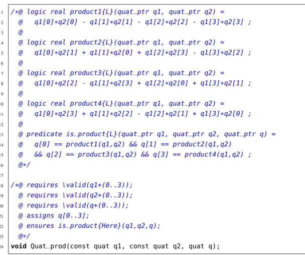
4.1.2. Multiplication of Quaternions
The next step is to specify the functionQuat_prodfor quaternion multiplica-tion. This is shown on Figure4. The predicateis_productis a direct transcription
of the mathematical formula defining the product of quaternions. The keyword
logic introduces definitions of additional first-order symbols to be used in anno-tations. The label Lis needed to make explicit that the defined expressions must be evaluated in some memory state: a construct \at(..., L) is implicit there. The contract forQuat_prodtells that the three given pointers should point to valid blocks in memory (lines 18-20), that only the block pointed by third pointerqis
/*@ logic real quat_norm{L}(quat_ptr q) = @ \sqrt(q[0]*q[0] + q[1]*q[1] + q[2]*q[2] + q[3]*q[3]); @*/ /*@ requires \valid(q+(0..3)); @ assigns q[0..3]; @ ensures quat_norm(q) == 1.0; @*/ void random_unit_quat(quat q);
Figure 5: Specification ofrandom_unit_quat int test1(void) {
quat current, next, incr; random_unit_quat(current);
/*@ loop invariant quat_norm(current) == 1.0; @*/
while (1) { ...
Figure 6: Specification of our main property
modified (line 21), and at the endqpoints to the product of the two other quater-nions (line 22).
4.1.3. Arbitrary unit quaternions
Next, we want to specify the random_unit_quat function, by saying that the result is of norm 1. This is shown on Figure5. The norm is introduced by a new logic functionquat_norm, making use of the ACSL built-in logic function symbol \sqrt denoting the square root. The contract of random_unit_quat says that the argument should point to a valid block, which is modified by the function, and contains at the final state some quaternion of norm 1.
4.1.4. The main loop
There is no need to specify our main functiontest1with a contract. Instead,
our expected property is naturally specified as a loop invariant in the body of the function. This is shown on Figure6.
Proof obligations Alt-Er go (0.95.1) CVC3 (2.4.1) CVC4 (1.0) Coq (8.4) Z3 (3.2) Z3 (4.3.1)
Lemma norm_product, lemma (5s) (5s) (5s) 2.43 (5s) (5s) VC for _Quat_copy_ensures_default 0.05 0.08 0.08 0.06 0.04 VC for _Quat_copy_safety 0.06 0.08 0.06 0.04 0.02 VC for _Quat_prod_ensures_default (5s) 0.11 0.08 0.06 0.04 VC for _Quat_prod_safety 0.05 0.08 0.06 0.04 0.04 VC for test1_ensures_default transformationsplit_goal_wp
1. loop invariant init 0.06 0.06 0.08 (5s) (5s)
2. assertion (5s) 0.10 (5s) (5s) (5s)
3. loop invariant preservation (5s) 0.14 (5s) (5s) (5s) VC for test1_safety 0.08 0.09 1.50 0.23 0.12
Figure 7: Infinite precision model, proof results
/*@ lemma norm_product{L}:
@ \forall quat_ptr q1,q2,q; is_product(q1,q2,q) ==> @ quat_norm(q) == quat_norm(q1) * quat_norm(q2); @*/
Figure 8: Lemma on the norm of a product 4.2. Proofs
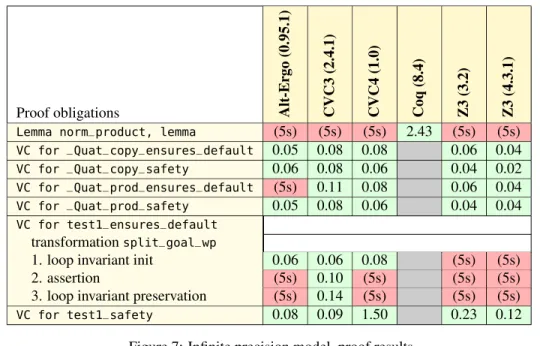
Our source code, annotated with ACSL specifications, is ready to be passed to Frama-C and the Jessie plugin. The resulting verification conditions and the results of the run of theorem provers are given on Figure7. A result of the form (5s) means that the prover was interrupted after a time limit of 5 seconds. The verification conditions named as “safety” concern extra properties, like validity of pointer dereference.
The proofs thatQuat_copyandQuat_prodsatisfy their specifications are easily done using automatic provers. The random_unit_quat is not implemented, only specified, so nothing has to be proved.
The only difficult proof is the test1 function. As such, the loop invariant cannot be proved preserved by the loop. This is because the property of the norm of a product is not known by automatic provers. We thus pose the lemma given
on Figure8, inserted as such in the source file. To help the prover, we also insert an intermediate assertion in the body of the loop, as follows:
while (1) { random_unit_quat(incr); Quat_prod(current,incr,next); //@ assert quat_norm(next) == 1.0; Quat_copy(next,current); } return 0; }
With the additional lemma and the intermediate assertion, the proof of our main function is made automatically. However, the lemma itself should be proved and no automated theorem provers is able to do it. There is no difficult reasoning step to perform it, only support for the square root function seems to be missing. To prove this lemma we run the interactive prover Coq. The proof is made with a few lines of tactics as follows. This proof makes use of thewhy3Coq tactic, which is able to call back again SMT solvers, through the Why3 intermediate system. The tactic must take as argument the name of the prover to apply. When the prover reports that the considered sub-goal is valid, the tactic makes this sub-goal an assumption in Coq. There is no Coq proof reconstructed by the tactic.
intros; unfold quat_norm.
rewrite <- sqrt_mult. (* sqrt(x*y) = sqrt(x) * sqrt(y) *) apply f_equal.
unfold is_product,product1,product2,product3,product4 in h1. ring_simplify; why3 "cvc3".
why3 "alt-ergo". why3 "alt-ergo".
This ends the verification using the infinite precision model. 5. Verification using the Floating-Point Model
We now switch back to the floating-point model used by default in the Jessie plug-in. Using this model, there is no change to make on the specification of the copy function Quat_copy, since there is no computation in this code. But this is not the case for other functions.
/*@ ensures distance_quat_vect(q,product1(q1,q2),product2(q1,q2), @ product3(q1,q2),product4(q1,q2)) <= EPS0; @*/
void Quat_prod(const quat q1, const quat q2, quat q);
Figure 9: Incomplete, updated specification of multiplication 1 /*@ logic real norm2(real p1, real p2, real p3, real p4) = 2 @ p1*p1 + p2*p2 + p3*p3 + p4*p4;
3 @
4 @ logic real norm_vect(real p1, real p2, real p3, real p4) = 5 @ \sqrt(norm2(p1,p2,p3,p4));
6 @
7 @ logic real quat_norm{L}(quat_ptr q) = 8 @ norm_vect(q[0],q[1],q[2],q[3]);
9 @
10 @ logic real distance2(real p0, real p1, real p2, real p3, 11 @ real q0, real q1, real q2, real q3) = 12 @ norm2(q0 - p0, q1 - p1, q2 - p2, q3 - p3) ;
13 @
14 @ logic real distance_quat_vect{L}(quat_ptr q, real p0, real p1,
15 @ real p2, real p3) =
16 @ \sqrt(distance2(q[0], q[1], q[2], q[3], p0, p1, p2, p3)) ; 17 @*/
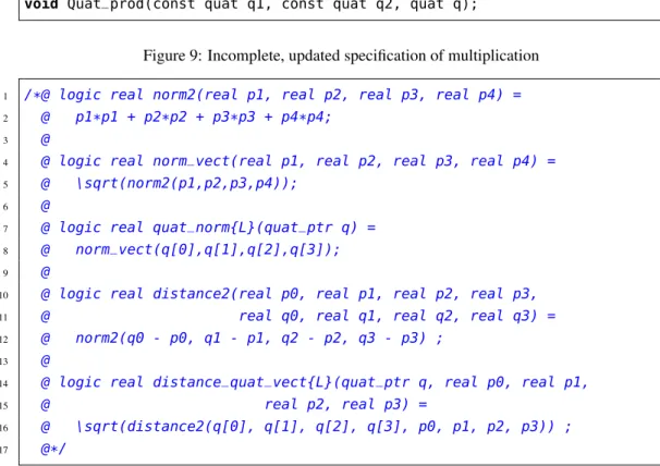
Figure 10: Formalization of the distance of two quaternions 5.1. Updated specifications
5.1.1. Rounding Error on Multiplication
In Section4, we prove that the C code forQuat_prodcomputes the quaternion multiplication. This was true and indeed trivial since an infinite precision was assumed. But this is not true anymore because of rounding. We need to find a way to specify that function differently: we express that the computed result is close to the infinite precision computation in real numbers, for some notion of distance to define. The new specification, incomplete for the moment, ofQuat_prodis shown
on Figure9. The value of theEPS0bound is given later. The post-condition makes use of an extra functiondistance_quat_vectthat is defined on Figure10.
difference. As a preliminary step, we redefine the norm of quaternions in several steps: first the square of the norm of a quadruple of real numbers (lines 1-2), then the norm of quadruple (lines 4-5), and last the norm of a quaternion (lines 7-8) as we did in Section 4, but using our intermediate definitions above. We then introduce the square of the distance of quadruples (lines 10-12), and finally the distance between a quaternion stored in memory and a quadruple of real numbers (lines 14-16), as used in the contract ofQuat_prod.
Our bound on the distance between the result of Quat_prod and the infinite precision product will allows us to later deduce a bound on the norm of the iterated product, thanks to the classical triangle inequality.
5.1.2. Estimation of the Rounding Error
The rounding error on the multiplication is the accumulation of errors when computing 16 floating-point multiplications and 12 additions or subtractions, in double precision. This rounding error is indeed proportional to the magnitude of numbers we have to multiply or add. In our case the numbers are components of unit quaternions so they are supposed to lie between−1 and 1. Nevertheless, since the accumulation of rounding errors introduces quaternions of a norm slightly larger than 1, the bound on the components is slightly larger than 1. We assume for the moment, and it will be validated later, that this norm remains smaller than β = 9
8.
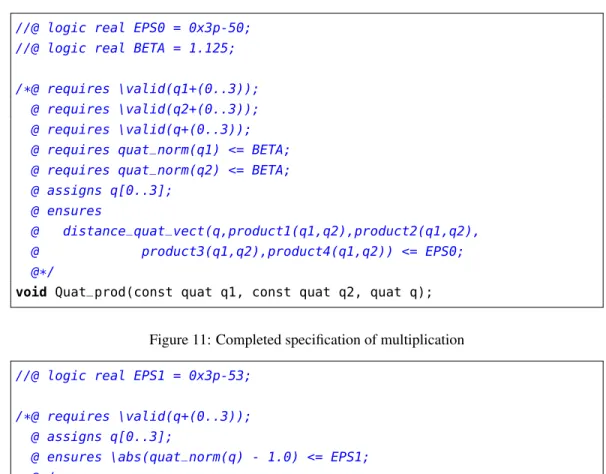
This bound on the quaternion components being chosen, a bound on the round-ing error on the quaternion multiplication can be found. To find this bound, we use the tool Gappa introduced in Section 3. The bound found by Gappa is ε0 = 3 × 2−50. Notice that even if we try to use a smaller bound than β =
9 8, the value ofε0 proposed by Gappa remains the same. The complete contract for function Quat_prod is given on Figure 11, with preconditions on the validity of
pointers in memory and other preconditions to bound their norm byβ. 5.2. Therandom_unit_quatfunction
It is not realistic to assume that therandom_unit_quatfunction returns a quater-nion of norm 1 exactly. Instead, we should assume that it returns a quaterquater-nion whose norm is close to 1 with some error boundε1. The new contract is shown on Figure12.
Our estimation ofε1 = 3 × 2−53was calculated by assuming that the returned quaternion was obtained by some arbitrary source, and then normalized, that is each of its components were divided by its norm. Of course our specifications are parametric with respect to this bound, which can be changed if needed.
//@ logic real EPS0 = 0x3p-50; //@ logic real BETA = 1.125; /*@ requires \valid(q1+(0..3));
@ requires \valid(q2+(0..3)); @ requires \valid(q+(0..3)); @ requires quat_norm(q1) <= BETA; @ requires quat_norm(q2) <= BETA; @ assigns q[0..3];
@ ensures
@ distance_quat_vect(q,product1(q1,q2),product2(q1,q2), @ product3(q1,q2),product4(q1,q2)) <= EPS0; @*/
void Quat_prod(const quat q1, const quat q2, quat q);
Figure 11: Completed specification of multiplication
//@ logic real EPS1 = 0x3p-53; /*@ requires \valid(q+(0..3));
@ assigns q[0..3];
@ ensures \abs(quat_norm(q) - 1.0) <= EPS1; @*/
void random_unit_quat(quat q);
Figure 12: New contract forrandom_unit_quat
5.3. Iterated product
The specification of our main property is given on Figure13. The value ofε is defined as the sum of the previous boundsε0 andε1. To express our property, we need to make explicit the number of iteration of the loop. It is done by a ghost variable n added in the code, on line 7. Notice that this ghost variable is a C long long. It would have been better to use an ACSL unbounded integer
but unfortunately the ghost variables are not allowed to be of a true logic type in Frama-C. We bound that numbernof iterations by a constantMAX, arbitrarily set to1010
for the moment. We discuss the value of this bound later. Notice that since the loop is infinite, the assertion on line 18 is not true, hence not provable in our verification process. We just ignore this unproved verification condition.
1 //@ logic real EPS = EPS0 + EPS1;
2 //@ logic integer MAX = 10000000000; // 10^{10} 3
4 int test1(void) {
5 quat current, next, incr; 6 random_unit_quat(current); 7 //@ ghost long long n = 1;
8 // an integer would be better, see text 9
10 /*@ loop invariant 0 <= n <= MAX;
11 @ loop invariant quat_norm(current) <= power(1.0 + EPS,n);
12 @*/ 13 while (1) { 14 random_unit_quat(incr); 15 Quat_prod(current,incr,next); 16 Quat_copy(next, current); 17 //@ ghost n++ ; 18 //@ assert n <= MAX ; 19 // not true, see text 20 }
21 return 0; 22 }
Figure 13: Specification of our main property 5.4. Proofs
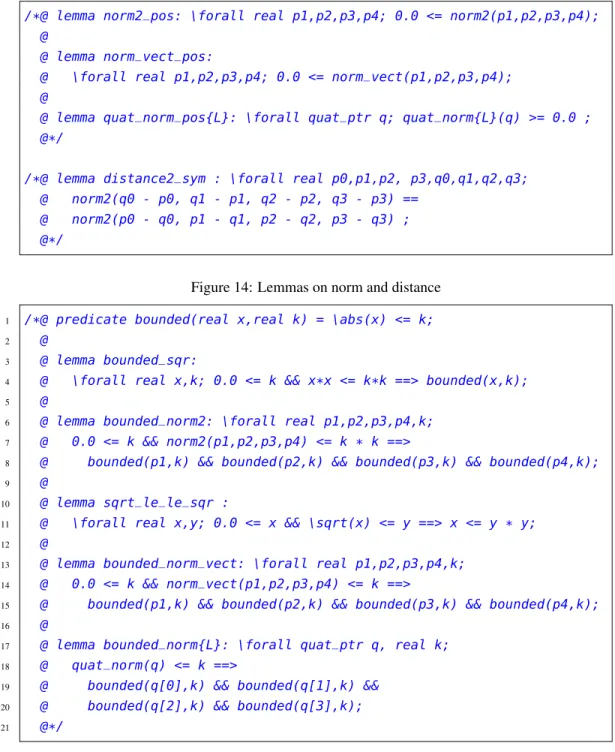
The proof of all the generated verification conditions is significantly more involved than in the infinite precision case. A first set of lemmas, shown on Figure 14, state that the norm is always non-negative, and then that distance is symmetric.
A next series of lemmas, shown on Figure15, are needed to establish that if a quaternion has a norm bounded by some constantk, then each of its components is bounded byk. These conditions on bounds on components are formalized using a predicateboundedsaying that the absolute value of real numberx is bounded by real numberk.
The proof results on these lemmas are shown on Figure16. The first series of lemmas (of Figure 14) can be proved automatically. The lemmas of the second series are also proved automatically, except the lemmabounded_sqrthat can only
/*@ lemma norm2_pos: \forall real p1,p2,p3,p4; 0.0 <= norm2(p1,p2,p3,p4); @
@ lemma norm_vect_pos:
@ \forall real p1,p2,p3,p4; 0.0 <= norm_vect(p1,p2,p3,p4); @
@ lemma quat_norm_pos{L}: \forall quat_ptr q; quat_norm{L}(q) >= 0.0 ; @*/
/*@ lemma distance2_sym : \forall real p0,p1,p2, p3,q0,q1,q2,q3; @ norm2(q0 - p0, q1 - p1, q2 - p2, q3 - p3) ==
@ norm2(p0 - q0, p1 - q1, p2 - q2, p3 - q3) ; @*/
Figure 14: Lemmas on norm and distance 1 /*@ predicate bounded(real x,real k) = \abs(x) <= k;
2 @
3 @ lemma bounded_sqr:
4 @ \forall real x,k; 0.0 <= k && x*x <= k*k ==> bounded(x,k);
5 @
6 @ lemma bounded_norm2: \forall real p1,p2,p3,p4,k; 7 @ 0.0 <= k && norm2(p1,p2,p3,p4) <= k * k ==>
8 @ bounded(p1,k) && bounded(p2,k) && bounded(p3,k) && bounded(p4,k);
9 @
10 @ lemma sqrt_le_le_sqr :
11 @ \forall real x,y; 0.0 <= x && \sqrt(x) <= y ==> x <= y * y; 12 @
13 @ lemma bounded_norm_vect: \forall real p1,p2,p3,p4,k; 14 @ 0.0 <= k && norm_vect(p1,p2,p3,p4) <= k ==>
15 @ bounded(p1,k) && bounded(p2,k) && bounded(p3,k) && bounded(p4,k); 16 @
17 @ lemma bounded_norm{L}: \forall quat_ptr q, real k; 18 @ quat_norm(q) <= k ==>
19 @ bounded(q[0],k) && bounded(q[1],k) && 20 @ bounded(q[2],k) && bounded(q[3],k); 21 @*/
Proof obligations Alt-Er go (0.95.1) CVC3 (2.4.1) CVC4 (1.0) Coq (8.4) Gappa (0.16.4) Z3 (3.2) Z3 (4.3.1)
Lemma norm2_pos, lemma 0.02 (5s) (5s) 0.00 0.06 0.04 Lemma norm_vect_pos, lemma 0.03 0.06 0.16 0.00 0.05 0.04 Lemma quat_norm_pos, lemma 0.04 0.09 0.16 0.00 (5s) 0.04 Lemma distance2_sym, lemma 0.03 0.06 0.08 0.00 0.04 0.01 Lemma bounded_sqr, lemma (5s) 2.02 (5s) 2.34 0.00 (5s) (5s) Lemma bounded_norm2, lemma (5s) (5s) (5s) 0.00 3.16 0.05 Lemma sqrt_le_le_sqr, lemma 0.03 (5s) (5s) 0.00 (5s) (5s) Lemma bounded_norm_vect, lemma 3.07 (5s) (5s) 0.01 (5s) (5s) Lemma bounded_norm, lemma 7.66 0.68 0.26 0.00 (5s) (5s) Lemma norm_product, lemma (5s) (5s) (5s) 3.80 0.00 (5s) (5s) Lemma pow_eps_max_int, lemma (5s) (5s) (5s) 4.33 0.00 (5s) (5s) Lemma power_monotonic, lemma (5s) (5s) (5s) 4.05 0.00 (5s) (5s) Lemma triangle_inequality, lemma (5s) (5s) (5s) 20.23 0.00 (5s) (5s) Lemma norm_distance_inequality, lemma (5s) (5s) (5s) 3.69 0.00 (5s) (5s)
Figure 16: Proof results on lemmas be shown in Coq (just 4 lines of tactics needed).
5.4.1. Proof ofQuat_prod
The functionQuat_prodcannot be proved as such, we have to give some extra annotations in the code, to help provers. The annotated code is given on Figure17. The series of assertions are needed because they will appear as hypotheses for Gappa when proving the bound on the rounding error. These assertions are proved by SMT solvers, which use the hypothesis that the norm is bounded.
The results of the proofs are shown on Figure 18. Notice that the post-condition is not proved directly, we have to split it: because it is made of the user’s post-condition (proved by Gappa) and the interpretation of the assigns
clause (proved by SMT solvers). Notice that there are also a lot of verification conditions generated to prove the absence of floating-point overflow in this code, not shown on the table. These are all proved by Gappa.
5.4.2. Proof of the main property
As for the product, our main function needs a few intermediate assertions to be proved. The corresponding annotated code is given on Figure19. The assertion on
void Quat_prod(const quat q1, const quat q2, quat q) { //@ assert bounded(q1[0],BETA); //@ assert bounded(q1[1],BETA); //@ assert bounded(q1[2],BETA); //@ assert bounded(q1[3],BETA); //@ assert bounded(q2[0],BETA); //@ assert bounded(q2[1],BETA); //@ assert bounded(q2[2],BETA); //@ assert bounded(q2[3],BETA); q[0] = q1[0]*q2[0] - q1[1]*q2[1] - q1[2]*q2[2] - q1[3]*q2[3]; q[1] = q1[0]*q2[1] + q1[1]*q2[0] + q1[2]*q2[3] - q1[3]*q2[2]; q[2] = q1[0]*q2[2] - q1[1]*q2[3] + q1[2]*q2[0] + q1[3]*q2[1]; q[3] = q1[0]*q2[3] + q1[1]*q2[2] - q1[2]*q2[1] + q1[3]*q2[0]; }
Figure 17: Annotated code of the multiplication function
Proof obligations Alt-Er
go (0.95.1) CVC3 (2.4.1) CVC4 (1.0) Gappa (0.16.4) Z3 (3.2) Z3 (4.3.1) VC for _Quat_prod_ensures_default transformationsplit_goal_wp 1. assertion 0.02 0.08 0.14 0.00 (5s) (5s) 2. assertion 0.05 0.08 0.15 0.00 (5s) (5s) 3. assertion 0.04 0.08 0.11 0.00 (5s) (5s) 4. assertion 0.04 0.08 0.14 0.00 (5s) (5s) 5. assertion 0.04 0.08 0.18 0.00 (5s) (5s) 6. assertion 0.04 0.08 0.30 0.00 (5s) (5s) 7. assertion 0.04 0.08 0.45 0.00 (5s) (5s) 8. assertion 0.04 0.09 0.88 0.00 (5s) (5s) 9. postcondition (5s) (5s) (5s) 0.07 (5s) (5s) transformationsplit_goal_wp 1. (5s) (5s) (5s) 0.11 (5s) (5s) 2. 0.04 0.13 0.13 0.10 0.12 1.09
1 int test1(void) {
2 quat current, next, incr; 3 random_unit_quat(current); 4 //@ ghost long long n = 1;
5 /*@ loop invariant 0 <= n <= MAX;
6 @ loop invariant quat_norm(current) <= power(1.0 + EPS,n);
7 @*/
8 while (1) {
9 random_unit_quat(incr); 10 Quat_prod(current,incr,next);
11 //@ assert quat_norm(incr) <= 1.0 + EPS1 ;
12 //@ assert quat_norm(current) <= power(1.0 + EPS,n) ; 13 /*@ assert quat_norm(current) * quat_norm(incr) <= 14 @ power(1.0 + EPS,n) * (1.0 + EPS1) ;
15 @*/ 16 Quat_copy(next, current); 17 //@ ghost n++ ; 18 //@ assert n <= MAX ; 19 } 20 return 0; 21 }
Figure 19: Annotated code of the main function
line 11 is just a reformulation of the post-condition of the call torandom_unit_quat,
just to simplify the Coq proof done later for the third assertion. The assertion on line 12 is a reformulation of the loop invariant after the product, posed for the same reason. The third assertion, on lines 13-14, is the one to help automated theorem provers. It is proved using Coq (in 4 lines of tactics), automated provers being too weak when dealing with multiplication. The proof results are given on Figure20.
Last but not least, five more lemmas were needed, shown on Figure21. The first lemma is analogous to the lemma on the norm of a product that we already posed for the proof in the infinite precision model. The only change is that the result of the product is expressed as a quadruple of reals instead of a
quat_ptr, because in this lemma we want to express a mathematical property on real numbers, not on floating-point ones.
Proof obligations Alt-Er go (0.95.1) CVC3 (2.4.1) CVC4 (1.0) Coq (8.4) Gappa (0.16.4) Z3 (3.2) Z3 (4.3.1) VC for test1_ensures_default transformationsplit_goal_wp
1. loop invariant init 0.17 0.16 0.11 0.00 (5s) (5s) 2. assertion (5s) 0.26 0.13 0.03 (5s) (5s) 3. assertion 0.04 0.09 0.18 0.03 0.06 0.02 4. assertion (5s) (5s) (5s) 2.40 0.03 (5s) (5s) 5. loop invariant preservation (5s) 0.31 (5s) 0.03 (5s) (5s)
Figure 20: Proof results for the main function
/*@ lemma norm_product{L}: \forall quat_ptr q1,q2;
@ \let p1 = product1(q1,q2); \let p2 = product2(q1,q2); @ \let p3 = product3(q1,q2); \let p4 = product4(q1,q2); @ norm_vect(p1,p2,p3,p4) == quat_norm(q1) * quat_norm(q2); @
@ lemma pow_eps_max_int: power(1.0 + EPS, MAX) <= BETA; @
@ lemma power_monotonic: \forall integer n,m, real x; @ 0 <= n <= m && 1.0 <= x ==> power(x,n) <= power(x,m); @
@ lemma triangle_inequality : \forall real p1,p2,p3,p4,q1,q2,q3,q4; @ norm_vect(p1+q1,p2+q2,p3+q3,p4+q4) <=
@ norm_vect(p1,p2,p3,p4) + norm_vect(q1,q2,q3,q4); @
@ lemma norm_distance_inequality: \forall real p1,p2,p3,p4,q1,q2,q3,q4; @ \sqrt(norm2(p1,p2,p3,p4)) <=
@ \sqrt(distance2(p1,p2,p3,p4,q1,q2,q3,q4)) @ + \sqrt(norm2(q1,q2,q3,q4));
@*/
call toQuat_prod, that require quaternions to have a norm smaller thanβ. This is
an assumption we made before, it is now the time to prove it.
The fourth lemma is the well-known triangular inequality, which is needed as an intermediate step for the fifth lemma, which in turn is needed to prove the preservation of the loop invariant. As shown on Figure16, all these lemmas must be proved in Coq. The first lemma is proved very similarly as in the infinite precision model, in a few lines of tactics.
The second and third lemma are quite simple on paper. Lemma
pow_eps_max_int is essentially a calculation. However it is a very complex one, and the only way we can prove it in Frama-C/Jessie is to use the intervaltactic
of Coq, as we need in our introductory example in Section3. The proof is only 2 lines long:
Strategy 1000 [powerRZ]. interval with (i_prec 39).
the parameters Strategy and i_prec are needed to increase the default precision and computing power of theintervaltactic. The lemmapower_monotonicis also
proved in Coq, using an induction on the variablem, in a few lines.
Although a classical result, proving the lemmatriangle_inequalityis not so easy, it is done in Coq. A classical proof amounts to prove first the Lagrange identity (X 1≤i≤4 a2 i) × ( X 1≤i≤4 b2 i) = ( X 1≤i≤4 aibi) 2 + X 1≤i<j≤4 (aibj − ajbi) 2
and then the Cauchy-Schwarz inequality X
1≤i≤4
aibi ≤ ||a|| × ||b||
Our Coq proof, that amounts to pose the two classical results above, prove them, and finally prove the lemma triangle_inequality, amounts to around 50 hand-written lines of Coq (using the why3tactic several times). Proving lemma norm_distance_inequalityis then done using 6 extra lines of Coq tactics.
5.5. Final remarks
We arbitrarily limited the number of iterations to 1010
. With this value, the bound we obtain on the norm of the iterated quaternionq is
which is only a small drift. It is easy to increase the maximal number of iterations
MAXto see how this bound evolves: the maximal number of interations for which we can still prove the program (in particular for lemmapow_eps_max_int) is more than 3.5 × 10¹³
iterations. Naturally, with this value the bound on the norm of quaternion q is getting close to 1.125, which may not be suitable for the appli-cation. Generally speaking, if we are given a required bound on the drift of the norm, we could determine the maximal number of iterations. Also, remember that those bounds depend on the bound assumed on the error on the norm of arbitrary quaternions taken as input. Changing the latter bound would change all the figures above.
A natural question is whether this bound is optimal or not. The answer is no. A first and clear reason is that the bound ε0 = 3 × 2−50 we found for the rounding error on a multiplication is already sub-optimal: this bound is provided by Gappa from the fact that each quaternion component qi is smaller than 1.125, meaning that the sum P
1≤i≤4q 2
i could be higher than 4, although we know in fact that it is lower than 1.1252
≃ 1.27. By hand, we can estimate that a three times smaller boundε0 = 2−50 would be correct too. A second reason is that the worst-case scenario corresponds clearly to a drift of the norm that is much higher than the drift obtained by a random source of input. It is thus desirable to employ probabilistic methods to evaluate the drift, that could tell what is the distribution of the norm after a given number of iteration, for a given distribution of inputs.
The last question is whether the worst-case bound obtained is useful from an industrial point of view. The first answer is yes because so far no such bound was known at all. Formerly, only random testing was performed, we now have a bound guaranteed sound in the worst case. It is not enough to completely forget about re-normalization of quaternions during the iteration, but it may permit to delay this re-normalization, e.g. this could occur once per second instead of at every step. The impact of a norm not being exactly 1 on the rest of the code remains to be analyzed too.
6. Related Work
Floating-point arithmetic has been formalized in deductive verification sys-tems since the mid 1990s: in PVS [34], in ACL2 [35], in HOL-light [36], in Coq [37]. These approaches were used to formalize abstraction of hardware com-ponents or algorithms, and prove some soundness properties. Examples of case studies are the formal verification of floating-point multiplication, division and square root instructions of the AMD-K7 microprocessor in ACL2 [35], and the
development of certified algorithms for computing elementary functions in HOL-light [36,38].
Proving properties related to floating-point computations in concrete C codes started a bit later, first within the Caduceus tool, using Coq for the proofs [39]. The support for floating-point in Frama-C/Jessie is inspired from this former work, and aims at a much higher degree of automation. A tutorial paper with several case studies was published [13], and public collections of verified C programs are pro-posed by the Hisseo project (http://hisseo.saclay.inria.fr/gallery.html), the Toccata research team (http://toccata.lri.fr/gallery/fp.en.html) and on S. Boldo’s web page (http://www.lri.fr/~sboldo/research.html). The most complex numerical case study so far using Frama-C is the numerical resolu-tion of a wave propagaresolu-tion differential equaresolu-tion, performed by Boldo et al. [40]. With respect to that case study, ours is hardly novel, since we both use Frama-C/Jessie. Yet, the case study of Boldo et al. makes a important use of Coq, whereas our quaternion case study takes care of using Coq only when no more automated solution are possible.
In an industrial context, the methods for proving properties of floating-point programs that got some good success belong to the class of abstract interpretation framework. In 2004, Miné used relational abstract domains to detect floating-point run-time errors [41], an approach that was implemented in the Astrée tool and successfully applied to the verification of absence of run-time errors in the control-command software of the Airbus A380. Another tool based on abstract interpretation is Fluctuat [42], a unique feature of it being the ability to provide comparison between executions of the same code in finite precision and in infinite precision.
Recently in 2013, Goodloe et al. [43] experimented with the verification of a C code implementing an automated air traffic control software that was formerly formalized in PVS [44]. Again, the specification amounts to relate finite compu-tation with infinite ones. Verification is done using Frama-C/Jessie and several provers including Gappa and PVS.
7. Conclusions and Perspectives
Specifying and proving a property on the functional behavior of a program involving floating-point computations can be achieved, but it is a complex activ-ity, that requires a good understanding and experience. Finding the proper way to express the specification already demands a significant level of expertise. The
proof itself can be obtained with a fair amount of automation, provided that sev-eral kinds of provers are available, and that the user has a good understanding of their respective abilities. Finding the appropriate mathematical lemmas is an issue. Specifying functional properties of floating-point programs typically in-volves bounds to put on inputs and outputs. Although Gappa can help to find such bounds, it remains essentially a human activity.
As our case study makes use of a lot of different tools (Frama-C, the Jessie plug-in, several provers) the question of the size of the trusted code base arises. This approach does not produce any kind of proof certificate at the end, that could be rechecked, so all the proof chain must be trusted. A crucial part is the inter-pretation of the semantics of the C code made by Jessie: there are known issues in that respect, due to the intricacies of the semantics of C (e.g. with respect to non-determinism of expression evaluation or pointer casting). Some progress was made recently to overcome this problem: a subset of ACSL was formalized on top of a formal semantics in C in Coq [45] and a corresponding verification condition generator for a subset of C was verified correct [46]. Nevertheless, on our case study the C code makes no use of any ambiguous C features, and the interpretation can be reasonably trusted, including the part on floating-point which is well doc-umented [22]. Another crucial part is raised from the fact that several provers are used to discharge the verification conditions. First, it should be trusted that they share the semantics interpretation of the logic formulas [23], and second each prover should be trusted, since they generally do not provide any proof certificate. In that respect, notice that Gappa can provide Coq certificates if needed.
Finally, an important general question is how to make the deductive verifica-tion of floating-point programs easier. If one wants to perform such a proof, we recommend as a first step to acquire some experience. This can be done by look-ing at other examples, such as the ones mentioned in Section6, and try to replay them. There is some future work that should make such an activity easier.
• Floating-point programs naturally rely on mathematical properties on real numbers. It is desirable to provide a rich set of mathematical notions and lemmas in a “standard library”. A typical example is the notion of vec-tors, dot product and norm, the triangle inequality property, etc. Specifying these from scratch like we did for this case study should not be the normal approach.
• An interesting question is whether the constraint solving process imple-mented by Gappa can be used as a decision procedure for the theory of
floating-point numbers inside a SMT solver. If this was done, then there will be no more need to insert intermediate assertions like the ones we added in theQuat_prodfunction.
• Increasing the degree of automation is another important issue. We had to use Coq to discharge several lemmas, related to properties on real numbers. Adding a support for a prover like Metitarski [32] that supports real expres-sions and elementary functions could be an important step.
• Another important issue in the verification of floating-point programs is the unstable tests: in case a program is making a test on a floating-point compu-tation, say testing whether a value if positive or not, then the behavior of the program can be very different than its idealized version using infinite preci-sion. In our case study, we have no branching in the code, so this problem did not show up. This issue deserves to be attacked specifically.
Acknowledgments. I gratefully thank the reviewers for their numerous sugges-tions for improving the paper. I also thank J.-L. Dufour and Ph. Baufreton from Sagem for providing the example and allowing me to publish the code, and G. Melquiond for his help in the use of both Gappa and theintervalCoq tactic. References
[1] The Frama-C platform for static analysis of C programs, http://www. frama-c.cea.fr/(2008).
[2] F. Bobot, S. Conchon, E. Contejean, M. Iguernelala, S. Lescuyer, A. Meb-sout, The Alt-Ergo automated theorem prover, http://alt-ergo.lri.fr/ (2008).
[3] S. Conchon, SMT techniques and their applications: from Alt-Ergo to Cu-bicle, Thèse d’habilitation, Université Paris-Sud, in English, http://www. lri.fr/~conchon/publis/conchonHDR.pdf(Dec. 2012).
[4] C. Barrett, C. Tinelli, CVC3, in: W. Damm, H. Hermanns (Eds.), 19th Inter-national Conference on Computer Aided Verification, Vol. 4590 of Lecture Notes in Computer Science, Springer, Berlin, Germany, 2007, pp. 298–302. [5] L. de Moura, N. Bjørner, Z3, an efficient SMT solver, in: TACAS, Vol. 4963
[6] G. Melquiond, Proving bounds on real-valued functions with computations, in: A. Armando, P. Baumgartner, G. Dowek (Eds.), Proceedings of the 4th International Joint Conference on Automated Reasoning, Vol. 5195 of Lec-ture Notes in Artificial Intelligence, Sydney, Australia, 2008, pp. 2–17. [7] Y. Bertot, P. Castéran, Interactive Theorem Proving and Program
Develop-ment, Springer-Verlag, 2004.
[8] P. Baudin, J.-C. Filliâtre, C. Marché, B. Monate, Y. Moy, V. Prevosto, ACSL: ANSI/ISO C Specification Language, version 1.4, http://frama-c.cea. fr/acsl.html(2009).
[9] Y. Moy, C. Marché, The Jessie plugin for Deduction Verification in Frama-C — Tutorial and Reference Manual, INRIA & LRI,http://krakatoa.lri. fr/(2011).
[10] Y. Moy, C. Marché, Modular inference of subprogram contracts for safety checking, Journal of Symbolic Computation 45 (2010) 1184–1211.
[11] J. Gerlach, J. Burghardt, An experience report on the verification of al-gorithms in the C++ standard library using Frama-C, in: B. Beckert, C. Marché (Eds.), Formal Verification of Object-Oriented Software, Papers Presented at the International Conference, Karlsruhe Reports in Informatics, Paris, France, 2010, pp. 191–204, http://digbib.ubka.uni-karlsruhe. de/volltexte/1000019083.
[12] J. Kuipers, Quaternions and Rotation Sequences: A Primer With Applica-tions to Orbits, Aerospace, and Virtual Reality, Princeton Univers. Press, 1999.
[13] S. Boldo, C. Marché, Formal verification of numerical programs: from C an-notated programs to mechanical proofs, Mathematics in Computer Science 5 (2011) 377–393.
[14] J.-C. Filliâtre, A. Paskevich, A. Stump, The 2nd verified software com-petition: Experience report, in: V. Klebanov, S. Grebing (Eds.), COM-PARE2012: 1st International Workshop on Comparative Empirical Evalu-ation of Reasoning Systems, EasyChair, Manchester, UK, 2012.
[15] V. Klebanov, P. Müller, N. Shankar, G. T. Leavens, V. Wüstholz, E. Alkas-sar, R. Arthan, D. Bronish, R. Chapman, E. Cohen, M. A. Hillebrand, B. Ja-cobs, K. R. M. Leino, R. Monahan, F. Piessens, N. Polikarpova, T. Ridge, J. Smans, S. Tobies, T. Tuerk, M. Ulbrich, B. Weiß, The 1st verified software competition: Experience report, in: M. Butler, W. Schulte (Eds.), FM, Vol. 6664 of Lecture Notes in Computer Science, Springer, 2011, pp. 154–168. [16] D. R. Cok, J. R. Kiniry, ESC/Java2 implementation notes, Tech. rep.,
http://secure.ucd.ie/products/opensource/ESCJava2/ESCTools/ docs/Escjava2-ImplementationNotes.pdf(may 2007).
[17] C. Bouillaguet, V. Kuncak, T. Wies, K. Zee, M. C. Rinard, Using first-order theorem provers in the Jahob data structure verification system, in: 8th In-ternational Conference on Verification, Model Checking, and Abstract Inter-pretation, Vol. 4349 of Lecture Notes in Computer Science, 2007, pp. 74–88. [18] L. Burdy, Y. Cheon, D. R. Cok, M. D. Ernst, J. R. Kiniry, G. T. Leavens, K. R. M. Leino, E. Poll, An overview of JML tools and applications, Inter-national Journal on Software Tools for Technology Transfer (STTT) 7 (3) (2005) 212–232.
[19] E. Cohen, M. Dahlweid, M. Hillebrand, D. Leinenbach, M. Moskal, T. San-ten, W. Schulte, S. Tobies, VCC: A practical system for verifying concurrent C, in: Theorem Proving in Higher Order Logics (TPHOLs), Vol. 5674 of Lecture Notes in Computer Science, Springer, 2009.
[20] M. Barnett, K. R. M. Leino, W. Schulte, The Spec# Programming System: An Overview, in: Construction and Analysis of Safe, Secure, and Interoper-able Smart Devices (CASSIS’04), Vol. 3362 of Lecture Notes in Computer Science, Springer, 2004, pp. 49–69.
[21] B. Carré, J. Garnsworthy, SPARK—an annotated Ada subset for safety-critical programming, in: Proceedings of the conference on TRI-ADA’90, TRI-Ada’90, ACM Press, New York, NY, USA, 1990, pp. 392–402.
[22] A. Ayad, C. Marché, Multi-prover verification of floating-point programs, in: J. Giesl, R. Hähnle (Eds.), Fifth International Joint Conference on Au-tomated Reasoning, Vol. 6173 of Lecture Notes in Artificial Intelligence, Springer, Edinburgh, Scotland, 2010, pp. 127–141.
[23] F. Bobot, J.-C. Filliâtre, C. Marché, A. Paskevich, Why3: Shepherd your herd of provers, in: Boogie 2011: First International Workshop on Interme-diate Verification Languages, Wrocław, Poland, 2011, pp. 53–64.
[24] J.-C. Filliâtre, A. Paskevich, Why3 — where programs meet provers, in: M. Felleisen, P. Gardner (Eds.), Proceedings of the 22nd European Sympo-sium on Programming, Vol. 7792 of Lecture Notes in Computer Science, Springer, 2013, pp. 125–128.
[25] IEEE standard for floating-point arithmetic, Tech. rep. (2008).
[26] D. Monniaux, The pitfalls of verifying floating-point computations, ACM Transactions on Programming Languages and Systems 30 (3) (2008) 12. [27] S. Boldo, T. M. T. Nguyen, Hardware-independent proofs of numerical
pro-grams, in: C. Muñoz (Ed.), Proceedings of the Second NASA Formal Meth-ods Symposium, NASA Conference Publication, Washington D.C., USA, 2010, pp. 14–23.
[28] S. Boldo, T. M. T. Nguyen, Proofs of numerical programs when the compiler optimizes, Innovations in Systems and Software Engineering 7 (2011) 151– 160.
[29] T. M. T. Nguyen, C. Marché, Hardware-dependent proofs of numerical pro-grams, in: J.-P. Jouannaud, Z. Shao (Eds.), Certified Programs and Proofs, Lecture Notes in Computer Science, Springer, 2011, pp. 314–329.
[30] T. M. T. Nguyen, Taking architecture and compiler into account in formal proofs of numerical programs, Thèse de doctorat, Université Paris-Sud (Jun. 2012).
[31] G. Melquiond, Floating-point arithmetic in the Coq system, Information and Computation 216 (2012) 14–23.
[32] B. Akbarpour, L. C. Paulson, Metitarski: An automatic theorem prover for real-valued special functions., Journal of Automated Reasoning 44 (3) (2010) 175–205,http://www.cl.cam.ac.uk/~lp15/papers/Arith/. [33] T. Hubert, C. Marché, Separation analysis for deductive verification, in:
Heap Analysis and Verification (HAV’07), Braga, Portugal, 2007, pp. 81– 93.
[34] V. Carreño, P. S. Miner, Specification of the IEEE-854 floating-point stan-dard in HOL and PVS, in: HOL95: 8th International Workshop on Higher-Order Logic Theorem Proving and Its Applications, Aspen Grove, UT, 1995. [35] D. M. Russinoff, A mechanically checked proof of IEEE compliance of the floating point multiplication, division and square root algorithms of the AMD-K7 processor, LMS Journal of Computation and Mathematics 1 (1998) 148–200.
[36] J. Harrison, Formal verification of floating point trigonometric functions, in: Proceedings of the Third International Conference on Formal Methods in Computer-Aided Design, Vol. 1954 of Lecture Notes in Computer Science, Springer, Austin, Texas, 2000, pp. 217–233.
[37] M. Daumas, L. Rideau, L. Théry, A generic library of floating-point numbers and its application to exact computing, in: 14th International Conference on Theorem Proving in Higher Order Logics, Edinburgh, Scotland, 2001, pp. 169–184.
[38] J. Harrison, Floating point verification in HOL Light: The exponential func-tion, Formal Methods in System Design 16 (3) (2000) 271–305.
[39] S. Boldo, J.-C. Filliâtre, Formal Verification of Floating-Point Programs, in: 18th IEEE International Symposium on Computer Arithmetic, Montpellier, France, 2007, pp. 187–194.
[40] S. Boldo, F. Clément, J.-C. Filliâtre, M. Mayero, G. Melquiond, P. Weis, Wave equation numerical resolution: a comprehensive mechanized proof of a C program, Journal of Automated Reasoning 50 (4) (2013) 423–456. [41] A. Miné, Relational abstract domains for the detection of floating-point
run-time errors, in: D. A. Schmidt (Ed.), 13th European Symposium on Program-ming (ESOP), Vol. 2986 of Lecture Notes in Computer Science, Springer, 2004, pp. 3–17.
[42] D. Delmas, E. Goubault, S. Putot, J. Souyris, K. Tekkal, F. Védrine, Towards an industrial use of FLUCTUAT on safety-critical avionics software., in: FMICS, Vol. 5825 of LNCS, Springer, 2009, pp. 53–69.
[43] A. Goodloe, C. A. Muñoz, F. Kirchner, L. Correnson, Verification of numer-ical programs: From real numbers to floating point numbers, in: G. Brat,
N. Rungta, A. Venet (Eds.), NASA Formal Methods, 5th International Sym-posium, Vol. 7871 of Lecture Notes in Computer Science, Springer, 2013, pp. 441–446.
[44] G. Dowek, C. Muñoz, Conflict detection and resolution for 1,2,...,N aircraft, in: Proceedings of the 7th AIAA Aviation, Technology, Integration, and Op-erations Conference, AIAA-2007-7737, Belfast, Northern Ireland, 2007. [45] S. Blazy, X. Leroy, Mechanized semantics for the Clight subset of the C
language, Journal of Automated Reasoning 43 (3) (2009) 263–288.
[46] P. Herms, Certification of a tool chain for deductive program verification, Thèse de doctorat, Université Paris-Sud,http://tel.archives-ouvertes. fr/tel-00789543(Jan. 2013).