Combining Laser Frequency Combs and Iodine Cell Calibration
Techniques for Doppler Detection of Exoplanets
K. Cahoy*
a, D. Fischer
b, J. Spronck
b, D. DeMille
ca
NASA Ames Research Center, Moffett Field, CA, USA 94035;
bYale University Dept. of Astronomy, New Haven, CT 06511;
c
Yale University Dept. of Physics, New Haven, CT 06511
ABSTRACT
Exoplanets can be detected from a time series of stellar spectra by looking for small, periodic shifts in the absorption features that are consistent with Doppler shifts caused by the presence of an exoplanet, or multiple exoplanets, in the system. While hundreds of large exoplanets have already been discovered with the Doppler technique (also called radial velocity), our goal is to improve the measurement precision so that many Earth-like planets can be detected. The smaller mass and longer period of true Earth analogues require the ability to detect a reflex velocity of ~10 cm/s over long time periods. Currently, typical astronomical spectrographs calibrate using either Iodine absorptive cells or Thorium Argon lamps and achieve ~10 m/s precision, with the most stable spectrographs pushing down to ~2 m/s. High velocity precision is currently achieved at HARPS by controlling the thermal and pressure environment of the spectrograph. These environmental controls increase the cost of the spectrograph, and it is not feasible to simply retrofit existing spectrometers. We propose a fiber-fed high precision spectrograph design that combines the existing ~5000—6000 A Iodine calibration system with a high-precision Laser Frequency Comb (LFC) system from ~6000—7000 A that just meets the redward side of the Iodine lines. The scientific motivation for such a system includes: a 1000 A span in the red is currently achievable with LFC systems, combining the two calibration methods increases the wavelength range by a factor of two, and moving redward decreases the “noise” from starspots. The proposed LFC system design employs a fiber laser, tunable serial Fabry-Perot cavity filters to match the resolution of the LFC system to that of standard astronomical spectrographs, and terminal ultrasonic vibration of the multimode fiber for a stable point spread function.
Keywords: exoplanet, astro-comb, laser frequency comb, Fabry-Perot, spectrograph, radial velocity, Doppler
1. INTRODUCTION
The discovery of more than 400 planets orbiting nearby stars has opened an exciting new subfield in astronomy with broad public appeal. The orbits of the ensemble of known exoplanets provide clues that have advanced our understanding of planet formation, evolution and migration (e.g., Juric & Tremaine 2007, Chatterjee et al. 2007, Ford & Rasio 2006, Fabrycky & Tremaine 2006 Ford & Chiang 2007, Armitage 2007, Alibert et al. 2005, Marzari et al. 2005, Kley et al. 2005, Ida & Lin 2004, 2005). For example, a preliminary comparison of the architecture of our own solar system to hundreds of other planetary systems suggests that Jupiter mass planets in wide circular orbits are not common (Marcy et al. 2008). While there are observational biases that favor the detection of close-in planets (Cumming et al. 2008), the next five years of Doppler (and microlensing) observations will provide important information about solar system analogs with gas giant planets beyond a few AU.
1.1 Gas Giant exoplanets are already being characterized
Unimaginable when the first few exoplanets were discovered, it is impressive that for the subset of transiting gas giant planets, it is possible to extract information about interior structure, planet atmospheres and co-planarity of orbits (Winn et al. 2009, Fortney et al. 2007, Torres et al. 2007, Burke et al. 2007, Bakos et al. 2007, Burrows et al. 2007, Chabrier & Baraffe 2007, Guillot & Showman, 2002). The Doppler measurements yield the mass of the planet and the photometric transit depth reveals the planet radius; together these data produce a mean density for the planet that constrains the planet core mass (Sato et al. 2005, Bodenheimer et al. 2003). HST spectroscopy has been used to identify atomic components in exoplanet atmospheres (Brown et al. 2001, Charbonneau et al. 2002). Spitzer infrared band photometry of primary and secondary eclipses has been used to measure the blackbody temperature of the planet and even to observe wind circulation in the atmosphere (Knutson et al. 2007).
With hundreds of gas giant planets already discovered, intense efforts are currently directed at the detection of small rocky planets like our own Earth. The scientific driver for this effort is the identification of potentially habitable planets (Lunine et al. 2008) Not every rocky planet is likely to host detectable life, so ideally, we would like to find many rocky planets.
1.2 How we can detect hundreds of Small Rocky planets with the Doppler method
The velocity amplitude for a small rocky planet depends on the separation from the host star and the mass of the host star. In the most favorable case of a close in rocky planet orbiting a low mass star, the velocity amplitude will be a few meters per second. However, a true Earth analog only induces a reflex velocity of 9 centimeters per second – 0.09 m s-1 – in a sunlike star. This is currently far below the single measurement precision of even the best Doppler precision; typical velocity precision ranges from a few meters per second to just below 1 m s-1 precision for the most stable spectrometers. Our strategy for obtaining centimeter per second precision is to: (1) Improve the single-measurement Doppler precision, and (2) obtain more data using a wider range of wavelengths per star to improve signal to noise (S/N) while mitigating the effects of stellar noise sources. We will describe an instrument that achieves 1 & 2 using a new design approach: extend and overlap the current 5000—6000 A Iodine calibration wavelength range with a scientifically motivated and technologically feasible Laser Frequency Comb from about 6500—7500 A. Our goal is to design a straightforward LFC-I2 calibration system that is compatible with a range of current and future spectrographs. Deployment at several sites will enable us to detect hundreds of small planets.
2. LFC-I2 COMPLEMENTS EARLIER LFC WORK AND OTHER EXOPLANET
DETECTION TECHNIQUES
Previous LFC work by Udem et al. (2002), Lovis et al. (2006), Murphy et al. (2007), Osterman et al. (2007), Li et al. (2008), Kim et al. (2008), Steinmetz et al. (2008) and others have developed the field significantly over the past few years. Their combined efforts have helped us to make design choices that address technical risks and promote a quicker path to science return. Some examples include our choices of a fiber laser, a redder and moderately narrow but scientifically motivated wavelength range, serial Fabry-Pérot cavity filters (Steinmetz et al. 2006, Steinmetz et al. 2009), trades between high reflectivity broadband GVD optimized and metallic (Au) mirrors, design of mirror curvature radii (Steinmetz et al. 2009) and terminal ultrasonic vibration of multimode fiber (Anderson et al. 1992).
2.1 LFC-I2 complements other exoplanet detection techniques
There are a few other techniques for detecting low mass planets, and we hope and expect that these techniques will be successful. Here we present only a couple of examples of other techniques that would be complemented by our proposed LFC-I2 work.
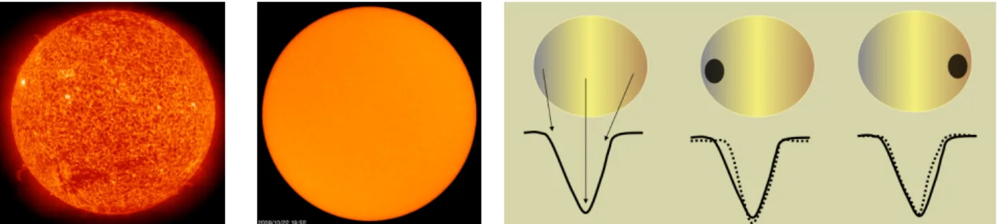
Figure 1: Images of the Sun taken on Oct 22, 2009 at blue wavelengths of 3040 A (left) and red wavelengths (central
wavelength 6780 A). Data are realtime images from SOHO EIT and MDI1. The surface contrast is clearly much greater for the blue wavelengths. As shown in the diagram on the right, because the star is rotating, with the approaching edge Doppler shifted to the blue and the receding edge Doppler shifted to the red, the disk-integrated stellar spectrum produce asymmetries in the spectral line profiles that can be misinterpreted as dynamical shifts in the center of mass.
1.0 0.8 0.6 0.4 0.2 0.0 5400 5402 541)4 5406 5408 5411) VvelerigIh IAJ
Kepler and other transit missions: the Kepler mission is now obtaining transit curves for roughly one thousand stars in
the Cygnus field (the Kepler field is much larger, but the search for transits of earth-radii planets will utilize a smaller subset of main sequence dwarfs). Doppler follow up will robustly identify gas giant planets, however, the detection of rocky planets requires a velocity precision of one meter per second. Because most Kepler stars are 100 – 1000 parsecs in distance, they are typically fainter than V=11. The faintness of the stars makes Doppler follow-up a challenging effort and it is likely that it will only be possible to establish masses for a few Earth-radii planets. For Kepler follow-up, radial velocity measurements are required to measure the planet masses and the LCF-I2 technique could help by increasing precision and signal-to-noise in the expanded wavelengths that are analyzed.
It is worth noting that transiting planets only comprise a thin slice of exoplanets; only about one in a thousand exoplanet architectures will present the nearly edge-on 90-degree orientations required to exhibit a transit. Nearly edge-on configurations are also more detectable with the Doppler technique (which measures the velocity amplitude times the sin of the orbital inclination), but a much wider range of inclinations are detectable: for an inclination of 45 degrees (the mean value for random orientations) or 60 degrees, the projected (line of site) velocity amplitude is only reduced to 70% or 87% (respectively) of the total velocity amplitude.
Space Interferometry Mission (SIM): Another technique for the detection of Earth-mass planets is space-borne astrometry (e.g. the Space Interferometry Mission). This technique will be particularly powerful for the closest stars. These are arguably the most interesting targets because proximity is critical for high signal-to-noise observations with future imaging missions. For the closest stars, space-borne astrometry may be more sensitive to dynamical motions than current ground-based Doppler observations (Makarov et al. 2009), although the I2-LFC aims to dramatically improve Doppler precision.
The LFC-I2 Doppler technique is complementary to space-borne astrometry because it will permit more effective prescreening of prospective mission targets and eventually assists with independent confirmation. While the sensitivity of space-borne astrometry decreases with distance, the Doppler technique can generally compensate for the faintness of distant stars with increased exposure times. So, the Doppler technique can add important information to support astrometric detections and reach more distant stars.
2.2 LFC-I2 will increase the chance of detecting large numbers of Small Rocky planets
The bottom line is that there are several techniques that will likely detect small rocky planets orbiting other stars. The question is: How many rocky planets do we want to find: a few, several, or hundreds? Kepler should find several, but will be limited to only a few confirmed masses until RV precision improves. Ground-based transit searches of low mass a) Fourier Transform Spectroscopy
(FTS) Iodine spectrum (b) Th-Ar (c) I2, Th-Ar, and LFC from Murphy et al. (2007)
Figure 2: Calibration line comparison. (a) The FTS Iodine spectrum shows a rich forest of molecular I2 lines, even after
it is convolved here with a typical LSF. (b) In contrast, the same 10-Angstrom wavelength band of Th-Ar contains only a few emission lines. The I2 spectrum is nearly uniform in intensity from 5000 – 6000 Angstroms. The Th-Ar spectrum spans the entire visible wavelength range (and beyond). (c) I2 and Th-Ar (2nd row, I2 red, Th-Ar black) and simulated LFC lines (3rd and 4th row) from Murphy et al. 2007.
stars should find a few, but will be limited by the number of accessible targets and the inclination requirement for a transit to occur. Space-borne astrometry could find several, but launch is uncertain. So, if the scientific goal is simply to detect a few Earth-like planets, existing projects and prospective missions should accomplish that goal.
2.3 LFC-I2 will increase the chance of detecting large numbers of Small Rocky planets
The bottom line is that there are several techniques that will likely detect small rocky planets orbiting other stars. The question is: How many rocky planets do we want to find: a few, several, or hundreds? Kepler should find several, but will be limited to only a few confirmed masses until RV precision improves. Ground-based transit searches of low mass stars should find a few, but will be limited by the number of accessible targets and the inclination requirement for a transit to occur. Space-borne astrometry could find several, but launch is uncertain. So, if the scientific goal is simply to detect a few Earth-like planets, existing projects and prospective missions should accomplish that goal.
3. BACKGROUND ON CURRENT DOPPLER CALIBRATION TECHNIQUES: I2 AND
TH-AR
3.1 The I2 calibration technique
The I2 Doppler technique makes use of an iodine cell, inserted into the light path before the spectrometer slit. As starlight passes through the cell, molecular iodine absorbs different frequencies of the light so that at the CCD detector, thousands of I2 lines are imprinted in the stellar spectrum. The information content of the I2 lines is extremely high – much richer than Th-Ar lines, as shown in Figure 2. The important attribute of this technique is that the iodine absorption lines (which serve as the wavelength calibrator and model the instrumental profile or LSF) travel through the identical path in the spectrometer as light from the star. This is critical because the I2 Doppler technique models the program observations (stellar observations through the iodine cell). The model is straightforward:
I2 × ISS ⊗ LSF = Observation
I2 = FTS iodine observation with R = 1,000,000 ISS = Intrinsic Stellar Spectrum LSF = Line Spread Function (a.k.a. PSF)
(Eq. 1)
We currently multiply a “perfect” I2 spectrum by the “perfect” intrinsic stellar spectrum and convolve that product with the LSF (which is a function of position on the detector) to achieve Doppler measurements with a precision of 1–2 m s-1. The limiting and interconnected factors for the precision of this technique are: (1) our ability to acquire a “perfect” intrinsic stellar spectrum (i.e., one deconvolved of the spectrometer LSF), and (2) our ability to determine the LSF. The LFC system will contribute to sampling and characterization of the LSFs. Since we have a nearly perfect FTS I2 spectrum (R = 1,000,000, SNR=2000), in principle we can model distortions (the LSF) in the I2 lines caused by imperfections in optics in the spectrometer. In practice this is complicated by variations in the slit illumination. We are addressing the critical problem of varying slit illumination now, by building and testing a fiber feed for the Hamilton spectrometer at Lick Observatory.
3.2 The Th-Ar calibration technique
The Th-Ar technique (e.g., HARPS2) is fundamentally different. At HARPS there are two fibers, one for the program star and one for the Th-Ar spectrum. The Th-Ar spectrum provides the wavelength solution, but it is spatially displaced from the stellar spectrum and Th-Ar emission lamps can change in intensity. This challenge has been admirably met at HARPS by construction of a spectrometer that is so stable (in temperature and pressure) that on spatial scales of picometers, nothing moves inside the spectrometer. Indeed, the spectrometer is so stable that the Th-Ar fiber can be “turned off” and relative shifts smaller than 1/1000th of a pixel are reliably measured by cross correlation, yielding precisions of about 1 m s-1. When multiple observations are averaged, the precision improves to about 0.8 m s-1. To achieve higher precision, a LFC is being tested at HARPS and has demonstrated precisions of tens of centimeters per second. Like the Th-Ar, the LFC will be fiber fed in parallel with the stellar spectrum.
3.3 Summary of current Doppler calibration differences, and how I2 in combination with LFC works
I2 spans 5000 – 6000 A of the spectrum; HARPS (Th-Ar) uses a wavelength range from about 4000 – 7000 A, effectively increasing the SNR in each observation. The LFC-I2 approach increases our wavelength range from 1000 to 2000 Angstroms. The spectrometer optics and CCD QE affect the I2 absorption lines in the same way as the stellar light. This is important for modeling the observations because whatever happens (e.g., broadening by the LSF) to the stellar
2High Accuracy Radial Velocity Planet Searcher
Figure 4: Starspot temperature contrast with respect to the photospheric temperature in active giants (squares) and
dwarfs (circles) from Berdyugina et al. (2005). Thin lines connect symbols referring to the same star. The thick solid line is a second order polynomial fit to the data excluding EK Dra. Dots in circles indicate solar umbra (delta T = 1700 K) and penumbra (delta T = 750 K).
lines also happens to the I2 lines. We think this approach is fundamentally correct and will inject the LSF into the science fiber and model the product of the absorption spectrum and emissions lines (accounting for differences in the brightness ratio of the star and LFC). In contrast, the Th-Ar lines are offset from the stellar lines – this challenge to Doppler precision was so great that the Th-Ar lines alone could not provide the RV precision at HARPS. The key to HARPS precision is extreme stability of the spectrometer. The demand for this pressure and temperature stability drives up the cost, essentially requiring a special-purpose spectrometer. In contrast, the I2 technique can be used with a general user spectrometer. However, to improve Doppler precision to better than 1 m s-1 greater stability will be needed, at least in the form of a fiber feed. We note that HARPS is fiber fed and an optical scrambler is used to produce a smooth and constant PSF.
4. SYSTEM DESCRIPTION
As noted in above, current calibration techniques involve passing the observed starlight through Iodine (I2) cells or using expensive and extremely stable spectrometers. The I2 lines are closely and fairly regularly spaced, but primarily over the 5000—6000 A range. As shown in Figure 2, the Th-Ar lines cover a wider range (about 4000—7000 A), but are more widely spaced, which leaves calibration gaps in high-resolution spectrographs. (Resolution R = λ/Δλ). For Doppler measurements to detect earthlike exoplanets, the spectrograph calibration needs to achieve a precision ~10 cm/s velocity shifts (~20 kHz frequency shifts) at optical wavelengths and maintain this accuracy over timescales of several years (due to the longer periods expected for earthlike planets). Without an external ultra-stable reference, long-term stability and environmental effects (thermal and mechanical) also affect the current calibration techniques. It is also difficult to directly compare measurements obtained with different instruments and at different times.
4.1 LFC-I2 and Starspots
A key consideration in the design and use of any spectroscopic instrument is the other limitation on Doppler measurements: stellar “noise.” Acoustic p-modes (pressure modes) cause the stellar atmospheres to oscillate, akin to seismic activity. These motions in the stellar surface can be misinterpreted as a dynamical motion when measuring Doppler shifts. The power spectrum of p-mode oscillations has been measured in the Sun; when the oscillations are in resonance, the amplitudes can be large as a few meters per second with periodicities of minutes (five minutes for the Sun). Because this source of stellar noise is high frequency, it is fortunately possible to average over asteroseismic noise with many observations or long exposure times.
More problematic, star spots can persist for one or more rotation periods. These spots are cooler, darker regions in the stellar photosphere, associated with magnetic loops. Young and rapidly rotating stars have stronger magnetic activity and are plagued by larger spots. In older stars like the sun, the spots are smaller and spot populations rise and fall with changes in activity cycles. The spot lifetime is proportional to the size of the spot, ranging from hours to weeks for our inactive Sun. This source of noise causes problems for Doppler measurements because a single spot can block light from the approaching edge of a rotating star. In an unresolved stellar disk, the blue edge of the spectral line loses some flux. When the spot then rotates with the star to the receding edge of the stellar disk, the red edge of the spectral line loses some flux. This periodic asymmetry in the shape of the spectral lines causes the line centroid to shift with the same rotation period as the star.
4.2 Starspot contributions are reduced at redder wavelengths
However, star spots are not completely dark and cold; they are typically 1000 K to 1500 K cooler than the surrounding photosphere (Figure 4). Therefore, the spot contrast (and stellar noise) is significantly reduced at redder wavelengths. The photosphere of the Sun has an effective temperature of 5770 K and sunspots have temperatures of about 4200 K. The peak emission for the Sun, according to Wien’s Law, is then at about 5100 A and the peak emission for sunspots is at about 7000 A. This suggests that the iodine region from 5000 – 6000 A (or HARPS spectra up to 6000 A) would still show significant spot contrast. This issue is illustrated by observations of the young star TW Hydra that showed periodic variability in visible wavelengths; these observations were misinterpreted as the detection of a Jupiter mass planet. However, Doppler observations made at infrared wavelengths (Huelamo et al. 2008), did not show any variability because the contrast between the stellar photosphere of TW Hydra and spots on the star was eliminated. The LFC-I2 approach, which targets a spectral region where starspots have lower contrast, can also benefit from collaborative ongoing work measuring and simulating the impact of starspots and stellar variability, e.g., Basu et al. (2007).
To emphasize the difference in starspot contrast with wavelength, images of the Sun taken at 3040 A are compared in Figure 1 with images of the Sun taken at 6780 A. Spot rotation can produce asymmetries that result in spurious Doppler shifts of hundreds of meters per second. This has precluded Doppler studies of young active stars in the past and
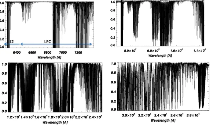
Figure 5: Spectra of the Earth’s atmosphere show large regions that are free of telluric lines between 6200 – 7400 A
(left upper) and 7400 – 10000 A (right upper). Spectra of the Earth’s atmosphere show more telluric lines in the infrared windows, 1.2 – 2.5 microns (left lower) and 2.5 – 4.0 microns (right lower).
motivated construction of infrared spectrometers which see low contrast stellar surfaces. Infrared Doppler measurements face their own set of challenges because telluric absorption lines from the Earths atmosphere litter the spectrum and literally change with the wind and column density of water at the level of 5 – 10 m s-1.
4.3 How the LFC-I2 design fits within telluric “windows
Telluric lines are spectral features caused by the Earth’s own atmosphere. The telluric spectrum is shown in Figure 5 for four wavelength segments. These figures show several “windows” that are comparatively free of telluric lines between 6200 A and 10000 A, and that longer wavelengths than about 1 micron have more significant telluric contributions. At
high resolution, many of the telluric lines can be masked out. Also, the convolution of these lines with the PSF means that in practice, the spectral features are shallower and broader than shown in Figure 5. However, working in telluric-free regions offers significant benefits.
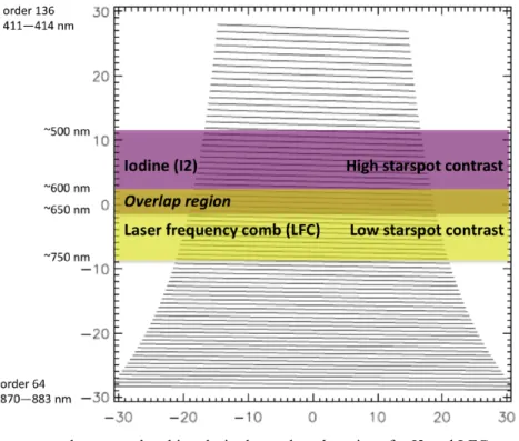
4.4 Overview of the LFC-I2 design
A combined I2 and LFC system that separately and simultaneously measures two spectral regions: 1. The 5000—6000 A spectral range of existing I2 calibration systems (
Figure 2
)2. The redder 6500—7500 A range which extends the spectral region towards wavelengths where influence from starspots is expected to be lower (Figure 1).
3. The design will include some spectral overlap, which will provide insight into the stability of the I2 system. 4. The wavelength regions covered contain “windows” in the telluric spectrum.
Figure 6: Sketch of the LFC-I2 system layout, as a concept that could be implemented on the CTIO Chiron
spectrograph. Light from the telescope is fiber-fed through the I2 system (which can be switched in or out), and then combined with light from the LFC system (which can also be removed from the path). The combined light is fed into the spectrograph. A separate pick-off of the LFC light will be used for monitoring of amplitude stability.
4.5 Calibration
This section describes some of the known calibration challenges and some steps that can be taken to address them. I2 calibration has a fairly constant intensity over an observation. We cannot currently assume the LFC intensity will remain constant over a few minutes to the levels needed, and so the plan is to monitor it across all wavelengths through the observation as shown in Figure 6. This can be accomplished by either feeding the LFC-I2 + starlight and the LFC separately into the spectrograph and using the inter-order spacing to monitor the LFC signal on its own, or alternatively, we can tap and redirect a small amount of the LFC light to a metering and feedback device. We propose to do both and evaluate the two approaches against each other. The LFC also offers a great way to sample and model the PSF, since its “teeth” are much narrower than I2. Each narrow “tooth” will convolve with and sample the PSF, and allow monitoring of asymmetries and distortions of the PSF. LFC characterization of PSFs will also be investigated during the integration of the LFC-I2 system with observatory facilities as part of this work.
4.6 The Laser Frequency Comb design
The overall LFC-I2 system layout is shown in Figure 6. Basics of the I2 system used were described in detail in the previous section. In this section, we focus on the design details and equipment necessary to implement the LFC part of the design.
4.7 Doppler precision estimates with LFC
Table 1 shows calculated estimates of the precisions possible with an LFC system for spectrographs like the in-progress CTIO Chiron or Keck HIRES . These precisions are estimated following the straightforward approach that was validated in Murphy et al. 2007. The pre-factor A in Table 1 represents the relationship between the functional form of the line profile and the relationship between S/N and pixel intensity. The value of 0.41 we use is taken from Murphy et al. 2007, where it was estimated for Gaussian line profiles with Poisson noise when photon noise dominates the detector noise. For the spectrograph with the 4096 x 4096 detector and S/N = 100, precisions of ~38 cm/s are estimated for a spectrograph with R = 80,000 as Chiron is projected to have. The precision for the 4096 x 4096 spectrograph improves to ~10 cm/s when S/N = 400.
Figure 7: Layout of the LFC portion of the LFC-I2 system. The 250 MHz Er fiber laser is referenced to an external
clock, such as RF synchronization with GPS time. The laser pulses at repetition rate fr of 250 MHz. This fr produces lines that are too dense for the resolution R of most spectrographs, so a Fabry-Pérot (FP) filtering assembly is used to increase the free spectral range (FSR) as in Steinmetz et al. 2009. Table 1 summarizes FSR values for a range of spectrograph resolutions following Murphy et al. 2007. The front-end of the system can be used to investigate several different approaches to the FP filtering assembly.
4.8 Achieving “comb tooth spacing” that matches spectrograph resolution
One area of research in LFC design is matching the comb resolution (FSR) to the spectrograph resolution. This is done using Fabry-Pérot filter cavities (Figure 6) to reduce the spectral resolution from the source to the spectral resolution R of the spectrograph being used. This means filtering the repetition rate from a 250 MHz fiber Er or Yb laser3 to achieve the FSR > 20 GHz needed for optical spectrographs with R > 60,000 (Table 2). We have selected a 250 MHz fiber laser (Er or Yb) since they are more stable and require less oversight during operation than the femtosecond Ti:Sa lasers. This filtering must also suppress all the other “teeth” by > 30 dB and span across the wavelengths of interest. The LFC-I2 design uses well-established I2 cells for calibrating the “bluer” part of the desired wavelength range. This reduces cost
3We propose a fiber Erbium laser at 250 MHz instead of a femtosecond Ti:Sa laser at ~1 GHz since the fiber lasers
Table 1 (a): Comparison of precision estimates for different resolution spectrographs with different CCD sizes
(calculations similar to those in Murphy et al. 2007).
and complexity by initially using a smaller wavelength range for the “redder” LFC calibration. This eases requirements on the spectral bandwidth of the Fabry-Pérot cavity filter assembly, which reduces system cost and complexity. For example, at 7500 A and an R ~ 80,000 spectrograph, a more reasonable “comb tooth” spacing of > 15 GHz is needed4, as shown in Table 2. For the same system designed to 4500 A, a more challenging FSR of > 25 GHz is needed.
4.9 LFC-I2 system also supports study of new and more complex LFC designs
The LFC-I2 approach also encourages pursuit of new and creative filtering designs to achieve higher FSR. Since the front-end of the LFC system (the fiber laser frequency comb) is separable from the FP “comb tooth” filtering on the back-end of the system, this goal is compatible as an extension of the LFC-I2 design (e.g., with different FP filtering strategies) in future iterations. As shown in Figure 6, the back-end of the system is separate and the FP filtering can be switched out to test different filtering schemes that optimize “comb tooth spacing” and “between-teeth suppression” for a variety of spectrograph resolutions that correspond to current or future observational facilities.
4 “Comb teeth spacing” FSR ~ 3 × c / (λ × R), where R is spectrograph resolution
Table 2: Free spectral range (FSR) as a function of wavelength and spectrograph resolution. For the LFC-I2 design,
we will achieve FSR > 20 GHz from 7000—8000 A. As shown in Table 3, our approach is to use FP filter cavities in series to reduce the requirements on finesse F while still achieving the needed mode spacing m.
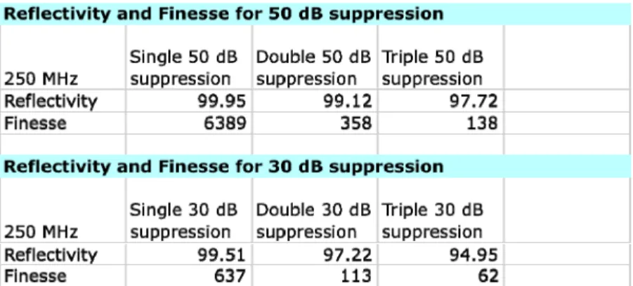
Table 3: Finesse and Reflectivity requirements for single FP cavity filter, “double” FP cavity filters in series, and
“triple” cavity filters in series (calculations based on Steinmetz et al. 2009). Requirements for 30 dB and 50 dB suppression are shown. We will first achieve 30 dB suppression and then attempt 50 dB suppression.
REFERENCES
[1] Alibert Y., Mordasini C., Benz W., Winisdoerffer C., A&A, 434, 343 (2005).
[2] Anderson, V.E., Fox, N.P., Nettleton, D.H., Applied Optics, Volume 31, Number 4, pp. 536-545 (1992). [3] Armitage, P,H, ApJ 665, 1381 (2007).
[4] Bakos, G.A. et al., ApJ 656, 552 (2007).
[5] Basu, S., Antia, H.M., Bogart, R.S., Astrophysical Journal, Vol. 651, 1146 (2007). [6] Berdyugina, S.V., Living Reviews in Solar Physics, vol. 2, no. 8 (2005).
[7] Bodenheimer P., Laughlin, G., Lin, D.N.C., ApJ 592, 555 (2003).
[8] Brown, T.M., Charbonneau, D., Gilliland, R.L., Noyes, R.W., Burrows, A., ApJ 552, 699 (2001). [9] Burke, C.J. et al., ApJ, 686, 1331 (2008).
[10] Burrows A., Hubeny, I., Budaj, J, Hubbard, W. B., ApJ 661, 502 (2007). [11] Chabrier, G. & Baraffe, I. ApJL 661, 81 (2007).
[12] Charbonneau, D., Brown, T.M., Noyes, R. W., Gilliland, R.L., ApJ 568, 377 (2002). [13] Chatterjee, S., Ford, E.B., Rasio, F. A., ApJ, 686, 580 (2008).
[14] Cumming, A. et al., PASP 120, 531 (2004) [15] Fabryky, D., Tremaine, S., ApJ 664, 1298 (2007) [16] Ford, E.B., Rasio, F. A., ApJ 686, 621 (2008) [17] Ford, E. B., Chiang, E. I., ApJ 661, 602 (2007)
[18] Fortney, J.J., Marley, M.S., Barnes, J. W., ApJ 659, 1661 (2007) [19] Guillot, T. & Showman, A., A&A, 385, 156 (2002)
[20] Huelamo, N., et al. Astronomy and Astrophysics, Volume 489, Issue 2, pp.L9-L13 (2008). [21] Ida, S., Lin, D.N.C., ApJ 616, 567 (2004)
[22] Ida, S., Lin, D.N.C., ApJ, 626, 1045 (2005). [23] Juric , M., Tremaine, S., ApJ, 686, 603 (2008).
[24] Kim, J., Cox, J.A., Chen, J., Kaertner, F.X., Nature Photonics, Volume 2, Issue 12, pp. 733-736 (2008). [25] Kley, W., Lee, M.H., Murray, N., Peale, S., A&A, 437, 727 (2005).
[26] Knutson H. A., Nature, Volume 452, Issue 7187, pp. 610-612 (2008).
[27] Lovis, C. et al., Ground-based and Airborne Instrumentation for Astronomy. Edited by McLean, Ian S.; Iye, Masanori. Proceedings of the SPIE, Volume 6269, pp. 62690P (2006).
[28] Lunine, J., editor, 2008, “Worlds Beyond: A Strategy for the Detection and Characterization of Exoplanets” Report of the Exoplanet Task Force to the Astronomy and Astrophysics Committee, arXiv:0808.2754v2
[29] Makarov, V.V. et al., ApJL (in press) [30] Marcy, G. W. et al., Phys. Scr. T130 (2008) [31] Mazari, F., ApJ 618, 502 (2008)
[32] McFerran, J.J., Applied Optics, vol. 48, issue 14, p. 2752 (2009).
[33] Murphy, M.T. et al., Monthly Notices of the Royal Astronomical Society, Volume 380, Issue 2, pp. 839-847 (2007). [34] Osterman, S. et al., Techniques and Instrumentation for Detection of Exoplanets III. Edited by Coulter, Daniel R. Proceedings of the SPIE, Volume 6693, pp. 66931G-66931G-9 (2007).
[35] Sato, B. et al., ApJ 633, 465 (2005).
[36] Steinmetz, T. et al., Applied Physics Letters, Volume 89, Issue 11, id. 111110 (2006). [37] Steinmetz, T. et al., Science, Volume 321, Issue 5894, pp. 1335- (2008).
[38] Steinmetz, T. et al., Applied Physics B, Volume 96, Issue 2-3, pp. 251-256 (2009). [39] Torres, G. et al., ApJL, 666, 121 (2007).
[40] Udem, Th., Holzwarth, R., Haensch, T.W., Nature, Volume 416, Issue 6877, pp. 233-247 (2002). [41] Winn, J. N. et al., ApJL 703, 99 (2009).