HAL Id: hal-01003840
https://hal.inria.fr/hal-01003840
Submitted on 10 Jun 2014
HAL is a multi-disciplinary open access
archive for the deposit and dissemination of
sci-entific research documents, whether they are
pub-lished or not. The documents may come from
teaching and research institutions in France or
abroad, or from public or private research centers.
L’archive ouverte pluridisciplinaire HAL, est
destinée au dépôt et à la diffusion de documents
scientifiques de niveau recherche, publiés ou non,
émanant des établissements d’enseignement et de
recherche français ou étrangers, des laboratoires
publics ou privés.
RTXP: A Localized Real-Time MAC-Routing Protocol
for Wireless Sensor Networks
Alexandre Mouradian, Isabelle Augé-Blum, Fabrice Valois
To cite this version:
Alexandre Mouradian, Isabelle Augé-Blum, Fabrice Valois. RTXP: A Localized Real-Time
MAC-Routing Protocol for Wireless Sensor Networks. Computer Networks, Elsevier, 2014, 67, pp.43-59.
�10.1016/j.comnet.2014.03.020�. �hal-01003840�
RTXP: A Localized Real-Time MAC-Routing Protocol for
Wireless Sensor Networks
∗Alexandre Mouradian, Isabelle Augé-Blum and Fabrice Valois
Université de Lyon, INRIA, INSA-Lyon, CITI, F-69621, France
[email protected]
ABSTRACT
Protocols developed during the last years for Wireless Sen-sor Networks (WSNs) are mainly focused on energy effi-ciency and autonomous mechanisms (e.g. self-organization, self-configuration, etc). Nevertheless, with new WSN appli-cations, new QoS requirements appear, such as time con-straints. Real-time applications require the packets to be delivered before a known time bound which depends on the application requirements. We particularly focus on appli-cations which consist in alarms sent to the sink node. We propose Real-Time X-layer Protocol (RTXP), a real-time communication protocol. RTXP is a MAC and routing real-time communication protocol that is not centralized, but instead relies only on local information. To the best of our knowledge, it is the first real-time protocol for WSNs us-ing an opportunistic routus-ing scheme in order to increase the packet delivery ratio. In this paper we describe the protocol mechanisms. We give theoretical bounds on the end-to-end delay and the capacity of the protocol. Intensive simulation results confirm the theoretical predictions and allow to com-pare RTXP with a real-time scheduled solution. RTXP is also simulated under harsh radio channel, in this case, the ra-dio link introduces probabilistic behavior. Nevertheless, we show that RTXP performs better than a non-deterministic solution. It thus advocates for the usefulness of designing real-time (deterministic) protocols even for highly unreliable networks such as WSNs.
Keywords
wireless sensor networks, real-time, MAC and routing pro-tocols.
1.
INTRODUCTION
A WSN is composed of nodes deployed in an area in or-der to monitor parameters of the environment. Those nodes are able to send information to dedicated nodes called sinks ∗This work has been partially founded by French Agence Nationale de la Recherche under contract VERSO 2009-017.
without the need of a fixed network infrastructure and in a multi-hop fashion. Every node is able to forward mes-sages from the other nodes. They usually run on batteries so they should consume as little energy as possible in order to increase the network lifetime. Because WSNs can con-tain thousands of nodes, the cost of a node should be as low as possible. This leads to design nodes with poor capa-bilities (computation, radio, memory, etc). In the past few years WSNs have been a very active research field which has led to interesting contributions at all communication layers. This is due to the great expectations put in WSN appli-cations. In fact, many applications have been proposed in the literature, such as volcano monitoring [32], air pollution monitoring [23], landslide detection [27] and so on.
Due to the previously mentioned characteristics of WSNs, network protocols have been designed mainly in order to reduce energy consumption and to provide autonomous net-work mechanisms. Nevertheless, some applications need more than these characteristics. Indeed, critical applications require more reliability and the respect of time constraints. For instance the aforementioned landslide detection applica-tion should give guarantees on the delivery of alert messages. Protocols which can deliver messages with guaranteed end-to-end delay are called real-time protocols. They are usually classified into two categories, soft time and hard real-time: in the first case, some messages can miss the deadline with no consequences (video) while in the second case, the delay constraint should be always respected whatever the circumstances because of the possible impact on human life, on the environment or on the financial cost. Due to the probabilistic nature of the radio links in WSNs, strict time constraint is not achievable, thus the time bound must be associated to a given reliability. This parameter is thus a main concern in the design of a WSN real-time protocol. Hard real-time constraints cannot be met with the current WSN protocols of the literature, either because of their lack of determinism which implies unbounded delays or low reli-ability, or because they do not take into account the afore-mentioned characteristics of WSNs.
In this paper, we propose a new localized real-time cross-layer protocol, RTXP. This protocol aims at giving a bound on the end-to-end delay in a WSN. In order to handle real-time requirements, deterministic mechanisms must be in-troduced at MAC and routing layers. The interactions be-tween these two layers must also be carefully controlled in
order to avoid unexpected and unbounded delays. We thus claim that a cross-layer design where MAC and routing lay-ers share information should be preferred. Our approach is to bound the duration of one hop1
and the number of hops to reach the sink. To avoid unbounded delays and unbounded route lengths, the access to the medium and the choice of the forwarder must be deterministic. Our approach is based on a suitable Virtual Coordinate System (VCS) [25]. This VCS allows the nodes to get information on their distance to the sink in number of hops. It also discriminates nodes hav-ing the same hop-counts in order to improve the forwarder selection. Finally, it gives a unique identifier to the nodes in an interference domain in order to deterministically access the medium. The VCS is constructed with local information (the neighbors of a node) and it is the only information used by RTXP. Our proposition is thus localized, no global view of the system is needed, the approach is therefore more scalable than centralized solutions. Moreover, RTXP uses an oppor-tunistic [9] routing scheme which allows to take advantage of transient links and thus to increase the reliability of the protocol. Under harsh channel conditions, no hard real-time guarantee can be given whatever the protocol used, because a message may need a very high number of retransmissions to be correctly transmitted (even if the probability of this event is low). Indeed, even if the protocol is deterministic, the radio link introduces probabilities in its behavior. In this paper, we show that a deterministic protocol allows to achieve better performances (notably reliability) than non real-time solutions.
In Section 2, we discuss the advantages and drawbacks of existing WSNs MAC and routing protocols for real-time ap-plications. In Section 3, we introduce the hypotheses and the requirements of our solution. In Section 4, we present the details of our proposition, RTXP. In Section 5, we give theoretical bounds on the end-to-end delay and the capacity of the protocol. Section 6 presents simulation parameters and results, we compare RTXP with a scheduled solution and a non real-time protocol. In Section 7, we conclude on the protocol properties and performances and we present our future works.
2.
RELATED WORK
A large number of WSNs MAC and routing protocols have been proposed during the last years. Unfortunately only few contributions focus on timeliness. In this section, we discuss the main results for MAC only, routing only and cross-layer protocols.
2.1
Medium Access Control
To save energy, MAC protocols for WSNs usually use a duty cycle [26] mechanism. Since the receiving, sending and lis-tening energy costs are approximately the same for usual radio chips [1], the only way to save energy is to turn off the radio (e.g. to switch to sleep mode). Duty cycling consists in nodes alternately waking up and going to sleep mode. MAC protocols can be classified into two main categories: synchronous and asynchronous. In synchronous protocols, the nodes know the schedules of the wakeup of other nodes [34] (in their neighborhood or in the whole network).
Usu-1We define the duration of one hop to be the time needed
for a node to access the medium and send a packet
ally a mechanism is used to synchronize the clocks of the nodes. They thus share a common global or local clock. In asynchronous protocols, the synchronization exists, but it is event-based: a communicating node and its neighborhood synchronize only for the time of a communication but with-out exchanging the values of their clocks. The technique used is called preamble sampling [26]: nodes pick a random wakeup time and then alternately sleep and wakeup. When it wakes up, a node senses the channel. If it detects energy it stays awake, otherwise it goes back to sleep. When a node needs to send a message, it sends a preamble (sequence of bits) which duration is equal to the duty cycle period be-fore sending the actual data packet, so all its neighbors stay awake. We can note that many improvements have been proposed in order to reduce the length of the preamble [11] [8] [18].
The channel access can be random or deterministic: in the first case the time to access the medium is not guaranteed because collisions can occur. This leads to unbounded delay to perform one hop, which is not suitable for real-time appli-cations. Solutions that provide deterministic access to the medium have been proposed in order to respect real-time constrains.
IEEE 802.15.4 [3] is a standard which defines a physical and MAC layer for WSNs. Networks can be peer-to-peer or star networks. In each case, at least one node acts as a coor-dinator and sends synchronization beacons. Between bea-cons, a superframe is defined. It is composed of two parts, Contention Access Period (CAP) and Contention Free Pe-riod (CFP). In the CFP, the accesses are guaranteed allow-ing real-time communications. This feature is used in the ISA100.11a [4] standard for wireless systems for industrial automation. Nevertheless, scalability [35] and reliability [7] issues have been highlighted. We can note that I-EDF [12] is another synchronous TDMA-based protocol which can give hard guaranties on medium access. The access to the time slots is based on Early Deadline First scheduling algorithm. The main issue of this proposition is its high energy con-sumption and the fact that nodes must be able to transmit on multiple channels.
On the contrary, f-MAC [28] proposes a localized and asyn-chronous approach. The principle is that nodes periodically send small packets (called frames) with a dedicated period, each node in the neighborhood having a unique period at-tributed. The authors show that, by applying mathematical rules for the choice of the periods, it can be guaranteed that a frame of each node will actually be transmitted without collision. This MAC guarantees hard real-time constraints on perfect radio links and the transmission mechanisms are very simple. Nevertheless, it has a very poor channel uti-lization, a quite high energy consumption (no duty cycle) and the maximum delay increases exponentially with the number of nodes in the same collision domain.
The MAC protocols described in this paper do not allow to respect strict time constraints (hard real-time) while taking into account the previously cited requirements specific to WSNs. The propositions which allow to respect hard time constraints do not take into account energy consumptions issues, radio chip limitations, or are difficult to integrate
with a routing layer. Other propositions are more suited to WSNs but do not allow to respect strict time constraints.
2.2
Routing
In this section, we focus on routing protocols for WSNs. They can be classified into four categories: probabilistic, hierarchical, location-based and opportunistic.
In probabilistic routing protocols, such as Random Walk Routing [30], forwarders are elected by making random choices. This class of protocols cannot be used for real-time commu-nications because of its lack of determinism. Indeed, it leads to unbounded routes length which do not allow to provide a bound on the end-to-end delay.
In hierarchical protocols, nodes can be grouped into clusters (as in LEACH [21]) or organized as trees (as in RPL [5]). In both cases, the structure guarantees that the length of the path to reach the sink is bounded, it can thus be used for real-time communications. Nevertheless, maintaining the structure can be expensive in terms of energy consumption in highly dynamic networks [6]. Moreover, in the case of a node failure, many nodes may result disconnected from the sink.
Location-based protocols are making forwarding decisions depending on the geographic location of the destination of the packet. A method for choosing a forwarder is to elect the neighbor of the sender which is the closest to the sink. SPEED [31] is a routing protocol based on geographic coor-dinates. A node keeps a table of its neighbors with a metric that represents their speed. The speed of a neighbor is com-puted by dividing the advance in geographic distance it pro-vides in direction of the destination by the delay to forward the packet to that neighbor. The forwarder is selected if its speed allows to respect the deadline of the forwarded packet. Nevertheless, SPEED does not bound the end-to-end delay. MMSPEED [20] increases the reliability of SPEED by us-ing a multi-path scheme. RPAR [15] enhances SPEED and MMSPEED by taking into account energy consumption and lossy radio links.
In opportunistic routing protocols, a node does not need to store explicit information on the network topology. It broad-casts the message and the choice of the next hop is done by nodes which receive it. The choice is based on a metric that can depend on the coordinates (geographic or virtual) and other parameters of the potential forwarders or it can be done randomly. GRAB [33] can be classified in this cate-gory of routing protocols. In GRAB the hop-count is used as a metric. Packets are routed using gradient-routing which consists in choosing the forwarder which has the lowest hop-count value. The advantages of such a solution are that the number of hops to reach the sink is known. Nevertheless, GRAB does not allow to discriminate nodes with the same hop-count. This information could be useful in order for example to select the best forwarder for a packet in a de-terministic way. SGF [22] and LQER [13] propose similar schemes. In SGF only one node is chosen in an opportunistic manner. LQER adds information on the link quality. Both solutions suffer from the same aforementioned drawbacks of GRAB.
Among the cited routing protocols, some take into account the time in order to route packets [31], others allow to bound the length of a route [34] or provide reliable end-to-end com-munications. Nevertheless, none is able to guarantee the respect of real-time constraints.
2.3
Cross-layer
Solutions which integrate both MAC and routing mecha-nisms have been proposed. These solutions allow to plan routes and medium access simultaneously.
PR-MAC [14] is a synchronous real-time MAC and routing protocol for WSNs. Its aim is to detect events and then to set up a periodical monitoring of the area where the event occurred. When an event is sensed in the network an alarm is sent to the sink. The sink responds with a packet that reserves a path for the periodical monitoring. The nodes on the path then wake up two times, once for the traffic from the source to the sink and once for the traffic from the sink to the source. The path is reserved with a given radio fre-quency. Once the path is reserved, the monitoring packets are transmitted in real-time but the reservation phase is non real-time and induces an overhead. Moreover the protocol assumes that the radio handles multi-channel communica-tions.
TSMP [17] uses a multi-frequency TDMA scheme to access the medium. It uses a centralized scheduling, where time-slots and channels are assigned to nodes in order to avoid interferences. The sink produces the scheduling which is sent to the nodes and executed.
PEDAMACS [19] also uses a scheduled approach, but with only one radio channel. Nodes have different transmission powers. The sink can reach all the nodes in the network. The other nodes have two transmission powers: one to com-municate and one to identify their interferers. The proto-col needs a global synchronization of the network. This is achieved thanks to synchronization packets that are sent by the sink to the whole network. The protocol consists of three phases. In the first one, the topology learning phase, each node learns its interferers and neighbors by sending hello packets in contention periods. During the second phase, the topology collection phase, the information is sent to the sink using a contention mechanism. A schedule is computed by the sink and sent to the nodes. The method used to produce the schedule is to linearize the graph of the network (contain-ing the interference edges) and to give the same color to non interfering levels. The slots are allocated to non-interfering sets of nodes with the same color. During the third phase, the nodes communicate in their allocated slots. RT-Link [29] uses a similar scheme: a global schedule is produced by the sink. Nevertheless, RT-Link uses a 2-hop heuristic in-stead of determining real interferers as in PEDAMACS. In RT-Link, the nodes are synchronized with an out of band scheme based on dedicated hardware added to the sensor nodes. We can notice that, unlike PEDAMACS, in RT-Link, CSMA/CA access slots allow to add new nodes in the schedule during the run-time of the protocol.
A drawback of centralized protocols is that the sink needs to retrieve information on the full topology of the network. This is not scalable and can lead to high energy consumption
and memory issues. In order to tackle these issues, LEMMA [24] proposes a distributed slot allocation mechanism based on the depth of a node in the routing tree and the real in-terferences among nodes. The allocation process is triggered by the sink. In a control slot, it proposes to allocate a slot to each of its children in the tree. In the proposed slot, a packet exchange allows to verify that no other pair of nodes uses it. A CSMA/CA access is used to detect possible interfer-ences. This process is repeated at every level of the routing tree. The protocol then switches to the steady-state mode in which the nodes access their slots in order to send and receive data. In this mode, the slots are still accessed with CSMA/CA in order to prevent new interferences and thus packet losses. Moreover, unlike PEDAMACS and RT-Link, LEMMA allows retransmissions during a time slot, it im-proves the reliability of the solution. The main drawback of LEMMA is that the slot allocation mechanism is not guar-anteed to converge in bounded time, this is due to the facts that the slots are accessed in a random way and also that the nodes may be randomly deployed.
In the remainder of this document, we present RTXP, a solution based on a deterministic and localized access scheme and opportunistic routing mechanisms.
3.
HYPOTHESES AND PROBLEM
STATE-MENT
3.1
Hypotheses
In this section, we discuss the assumptions we consider. As-sumptions we make are mainly related to the sensor capabil-ities, the radio environment and the application. Moreover, our proposition is based on more specific requirements. Assumptions on the limited capacities of sensor nodes:
• Sensors have a limited amount of energy; • The nodes have a limited amount of memory. Assumptions linked to the radio:
• The radio is half-duplex and mono-channel;
• We assume a 2-hop interference model, meaning that nodes are able to receive packets from their 1-hop neigh-bors and to detect activity of their 2-hop neighneigh-bors. We will discuss this assumption in the performance evaluation section (Section 6);
• Radio links are symmetric. Assumption linked to the application:
• The traffic intensity is low and consists in alarm pack-ets converging toward the sink;
Assumption more specific to our propositions:
• Nodes have local coordinates which give information on the number of hops from the sink and which are unique in an interference domain. This can be pro-vided by a solution we proposed in [25].
3.2
Problem statement
The goal of this work is to propose a real-time alarm gather-ing solution in WSNs in the context given by the hypothe-ses listed above. The solution must respect the following requirements:
• the protocol must ensure that the end-to-end delay is lower than a given bound;
• it must be scalable due to the large scale of WSNs; • it must be reliable because the applications are critical
and the wireless links are unreliable;
• it must be energy efficient because nodes run on bat-tery.
We propose to check that our solution fulfills these require-ments by evaluating its performances by simulation. For verifying that RTXP is able to respect timing constraints, we simulate the protocol operation and observe the end-to-end delays. In order to check the scalability of our propo-sition, we run simulations with networks of increasing size and observe how it influences the performances. We eval-uate the delivery ratio of RTXP in order to control its re-liability, and we evaluate its energy efficiency by observing the energy consumption during the simulations. Finally, we compare RTXP with existing protocols in order to highlight its contributions to the real-time alarm gathering problem in WSNs.
4.
PROPOSITION: A NOVEL REAL-TIME
X-LAYER PROTOCOL, RTXP
In this section we detail RTXP, a cross-layer (MAC and routing) protocol which guarantees a bounded end-to-end delay for alarm packets. We first give the general ideas of the protocol, we describe the virtual coordinate it uses as a metric, we detail further the mechanisms of the protocol and we characterize the supported traffic load in function of the parameters of the radio.
4.1
General idea
As energy is a main concern in WSNs, RTXP uses a duty cycle mechanism. We call awake period the period in which the nodes are awake and sleep period the one in which they turn off their radio.
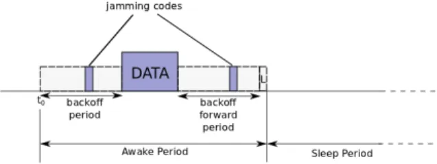
Figure 1: Description of the proposition As depicted in Figure 1, the awake period is divided into three main phases:
• A backoff period in which nodes with a packet in their queue contend to reserve the channel. The contention occurs among nodes of the same interference domain. Each node has a backoff timer that is calculated from its coordinate and is unique in the interference domain. During the backoff, the nodes sense the channel. Then, either the node’s backoff expires and the node sends a jamming code, meaning that it gains access to the channel, or it detects a jamming code before the end of its backoff timer (meaning that it loses the contention). • A time slot during which the data packet is
transmit-ted.
• Another backoff period during which all the nodes that received the data packet contend to forward it. This backoff period works the same way as the one for chan-nel reservation.
During the L slot, any node that lost the contention for the channel can send a jamming code which triggers a new awake period for the nodes that detect it. As it will be discussed in Section 4.3, and thanks to the uniqueness of the coordinate in an interference domain, the access to the channel and the selection of the forwarder are deterministic.
4.2
Wakeup time: preambles versus
synchro-nization
In the previous subsection, we assume that all the nodes of a given interference domain are awake at the beginning of the first backoff period noted t0. There are two ways of
achieving this goal (both can be used to implement RTXP). The first is by using a long preamble as in [26]. This solution does not need to maintain a global synchronization of the nodes. Nevertheless, the emission of the preamble consumes energy and time. Indeed, when an alarm converges toward the sink, each relaying node must send the preamble before executing the three phases presented in previous subsection. The second way is to have a global synchronization [29] of the nodes of the network so that all the nodes can wake up at the same time. Moreover, with global synchronization, a packet can be forwarded several times during a duty cycle, which reduces the average end-to-end delay. We choose to use a global synchronization for RTXP. So for the remainder of this paper we assume that the nodes of the WSN are syn-chronized with dedicated hardware as in [29]. Nevertheless, both schemes can be used to implement RTXP.
4.3
Virtual coordinate system
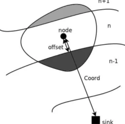
The Virtual Coordinate System (VCS) used by RTXP con-sists in a 1-D coordinate, which we proposed in a previous work [25]. The VCS is based on two parameters. The first one is the hop-count to the destination node, but since many nodes can have the same hop-count, we refine this param-eter with a second one. The nodes having the same hop-count can be seen, conceptually, as forming concentric rings centered on the sink. The second parameter represents the logical position of the node within a ring (noted offset) it is calculated in function of the repartition of its neighborhood among the different hop-count rings. Nodes having more
neighbors in proportion in the rings nearer to the sink are classified before nodes having more neighbors in proportion in the rings further from the sink. This information allows to give priority to nodes more connected to lower rings during the routing process.
Figure 2 illustrates the coordinate, the offset is the refine-ment of the hop-count (c.f. [25] for more details) and n is a ring number. In [25], the probability of having two nodes with the same coordinate in an interference domain is low but not null (this issue is discussed in [25]). In this paper we assume that the coordinate is unique in an interference domain.
Figure 2: Conceptual view of the 1-D coordinate used by RTXP
The coordinate initialization algorithm presented in [25] runs in bounded time (the bound depends on the maximum hop-count of the considered network). It is thus applicable in the context of real-time applications.
We can remark that any metric which provides the hop-count and which allows to discriminate the nodes in an in-terference domain can be used with RTXP.
4.4
In-depth detail of RTXP
First, we describe further the three phases of the protocol mentioned in Section 4.1.
Phase 1. In the first backoff period, each node being awake and having a packet to send contends for the channel. Dur-ing the contention, a node senses the channel. If it detects energy on the channel before the end of its backoff timer, it loses the contention. Otherwise, it sends a jamming code. A jamming code is a short sequence of bits, possibly ran-dom. The technique is very similar to preamble sampling [26], but with the jamming code being shorter than a typ-ical preamble. If a node loses the contention, it can notify the loss in a dedicated slot (noted L for Lost in Figure 1), by sending a jamming code in the slot. Every node that receives a jamming code in the L slot will stay awake for another awake period. As mentioned previously, we assume that the nodes are able to detect jamming codes from their 2-hop neighborhood in order to prevent the hidden termi-nal problem. The backoff timer is calculated with a bijective function from the coordinate (for example the offset is
trans-lated directly into milliseconds so the function is of the type y = x). The lemma 4.1 ensures that there is no collision in an interference domain.
Lemma 4.1. If the coordinates are unique in an interfer-ence domain and the backoff function is bijective then there is only one node that wins the contention.
Proof. We do a proof by contradiction. Let’s suppose there are two nodes that win the contention (i.e. there is a collision). That means they have the same backoff time which implies that either they have the same coordinate or the backoff function is not bijective which is a contradic-tion.
.
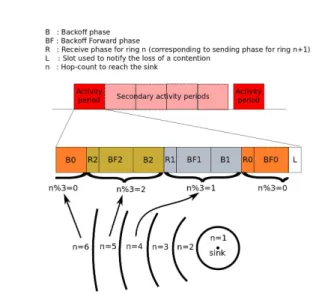
Figure 3: Description of the proposition Phase 2. During the second phase (data emission and re-ception), the node (with hop-count n) who won the con-tention of the first phase sends its packet and the nodes in range, with hop-count n − 1, receive it.
Phase 3. The third phase is another contention period (backoff forward phase). All the nodes that received a packet in the second phase contend to know which one will forward it. As in the first phase, the backoff function is bijective and calculated from the coordinate. We can notice, in this case, that we want to preserve the order given by the coordinate, thus the function must also be strictly monotonic. The first node whose backoff ends, sends a jamming code to notify the others that it will be the forwarder. We can notice that this mechanism is an opportunistic forwarding scheme based on the coordinate.
Organization of the phases. As said in Section 4.2, we choose to use a global synchronization scheme. This allows to forward a packet several times during one duty cycle be-cause potential forwarders are already synchronized. We also mentioned that we assume a 2-hop interference model, meaning that nodes that are three hops away can transmit at the same time. Thus, to give a chance to each node to
transmit during a duty cycle, whatever its hop-count, we should define three awake periods per duty cycle (but we keep only one L slot), one for nodes with 3j hop-count, one for 3j + 1 and one for 3j + 2 with j ∈ N. As depicted in Fig-ure 3, an activity period is composed of three awake periods. A packet can, at most, reach a node with 3j hop-count from a node with a 3j + 3 hop-count during one activity period. We can note that in the case that the 2-hop interference model hypothesis does not hold, it is possible to implement RTXP : for a N -hop interference model, nodes N hops away can be active at the same time.
Figure 3 depicts the different phases for nodes with differ-ent hop-counts. Bi, Ri and BFi correspond respectively
to backoff, receive and backoff forward phases with i = n mod 3. For example, a node 6 hops away from the sink contends in B0if it has a packet to send. It sends the packet
in R2if it wins the contention. It wakes up in R0to
poten-tially receive a packet and, if it has received one, it executes the BF0 phase to try to forward the packet.
When a node, which has a packet to transmit, loses the contention during the backoff phase, it has the opportunity to claim a new activity period (named secondary activity period ). This new activity period follows the previous one, without sleeping time. Only nodes which sense a jamming code in the L slot stay active. This allows to all the packets to do at least one hop toward the sink during a duty-cycle. This property is used in Section 5 in order to compute the theoretical bound on the end-to-end delay.
In WSNs, links are unreliable, the nodes may experience fading and shadowing. Thus, packets may not be correctly received. In order to mitigate the impact of unreliable links, we use an opportunistic routing scheme: data packets are broadcasted, and thus received by several nodes. The for-warder is elected during the BF phase. Moreover, the jam-ming code sent during the election of the forwarder (BF phase) is used as an acknowledgement. A node which sends a packet in the R phase then waits for a jamming code, if it does not receive one, the packet is considered lost and the node sends a jamming in the L slot to request a new activity period. The packet is resent in the new activity period. Example. The Figure 4 shows an example with a simple network. Nodes A and B both have data to send to the sink at the beginning. They contend in the first part of the activity period. B wins the contention, so it can send its packet in the R phase to C. Similarly, C sends it to D, and D then forwards it to the sink. At the end of the first activity period, node A sends a jamming code in the L slot because it has lost the contention to access the medium. Because we assume a 2-hop interference model, B, C and D sense the jamming code so they stay awake for a new activity period. In this second activity period, only A has a packet to send, thus A wins the contention and the packet is forwarded to C. At the end of the second activity period all the nodes go to sleep mode because no node transmits during the L slot (every packet has done at least one hop).
5.
THEORETICAL ANALYSIS
In this section, we derive the theoretical bound on the end-to-end delay named Worst Case Traversal Time (WCTT).
Figure 4: Example considering 4 nodes where nodes A and B have a packet to transmit
We also establish the real-time capacity of RTXP, which reflects the amount of traffic the protocol can serve while respecting the WCTT.
5.1
Delay, capacity and energy
In order to compute a bound on the end-to-end delay, we propose to calculate the worst duration for one hop and multiply it by the maximum number of hops in the network. We start by defining intermediate delays. The notations used in this section are detailed in Table 1.
B and BF durations depend on the backoff duration, which is function of the offset (backoff = f (offset)). Indeed, each node must have the possibility to send a jamming code dur-ing the period, so the duration of the backoff phases must be equal to the maximum backoff duration plus the duration of a jamming code:
DB = DBF= max(backoff ) + Djamming (1)
The R phase duration is the time required to transmit a data packet (noted DR). In our case, the data packet is an
alarm packet whose size is in the order of magnitude of a few dozens bytes.
The duration of the L slot (DL) is equal to the duration of
a jamming code (Djamming).
In order to determine the WCTT, we have to compute the length of the activity period and the sleep period. The sleep period duration (Dsleep) is calculated based on the time a
given node actually spends awake during an activity period noted Dawake, and on the duty cycle ratio noted DC. First
we have to notice that a node does not spend the whole activity period awake: it stays awake only for one B phase
plus one BF phase plus two R phases (one to send data to lower hop-count neighbors and one to receive data from up-per hop-counts nodes). Dsleepis thus determined as follow:
DC = Dawake/(Dsleep+ Dawake) (2)
Dawake= DB+ DBF+ 2 × DR+ DL (3)
Dsleep= Dawake× (
1
DC − 1) (4) The duty cycle ratio typically depends on the application characteristics, this aspect is discussed in Section 5.2. The activity period is represented in Figure 3, its duration is given by:
Dactivity period = 3 × (DB+ DBF+ DR) + DL (5)
The worst case duration for one hop is given by Dactivity period+
Dsleep because a packet, in the worst case, is transmitted
after having lost the contention every time until the limit given by the end of the sleep period. In order to give the WCTT, we have to multiply the worst case for one hop by the maximum number of hops in the network. We actually take the maximum number of hops plus one because there is a delay (which is at most one duty cycle period) between the instant the event is sensed and the first emission of the corresponding packet. So the WCTT, corresponding to the maximum end-to-end delay is given by:
W CT TRT XP = (N Bhop max+ 1) × (Dactivity period+ Dsleep) (6)
The number of activity periods (the first where all nodes wake up and secondaries triggered only if needed) is limited
symbol signification
DB Duration of the backoff (B) phase
DBF Duration of the backoff forward (BF ) phase
DR Duration of the receive (R) phase
DL Duration of the L slot
Djamming Duration of the jamming code
Dactivity period Duration of an activity period
Dawake Time a node spends awake during an activity period
Dsleep Duration of the sleep period
W CT TRT XP Theoretical bound on the end-to-end delay for RTXP
DC The duty cycle ratio CRT XP Capacity of RTXP
N Bhop max The maximum number of hops from the sink
Ebackof f Energy consumed during the backoff (B) phase
Ebackof f f orward Energy consumed during the backoff forward BF phase
ET X jamming Energy consumed during the emission of a jamming code
ET X packet Energy consumed during the emission of a packet
ERX packet Energy consumed during the reception of a packet
E1hop RT XP Energy consumed by RTXP to do one hop
Table 1: Notations used in the description of RTXP
by the length of the sleep period (which depends itself on the duty cycle value). We define the capacity of RTXP (CRT XP)
as the number of packets that can be transmitted into an interference domain during the duty cycle. Given the duty cycle duration (Dactivity period+ Dsleep), the capacity is:
CRT XP = ⌊
Dactivity period+ Dsleep
Dactivity period
⌋ (7)
Theorem 5.1. Let n ∈ N and p ∈ N be respectively a hop-count number and the number of packets in an interference domain at hop-count n. Assuming that packets can only be lost because of collisions, all packets in every interference domain at hop-count n will reach hop-count n − 1 in at most a duty cycle period if p < CRT XP.
Proof. We do a proof by contradiction. Let’s suppose one packet did not reach hop-count n−1 in one duty cycle pe-riod. Then either the packet was lost or it was delayed until the end of the period. As we assumed the only way to lose a packet is because of a collision. By lemma 4.1 we know that it is not possible, so it is a contradiction. If the packet is de-layed until the end of the duty cycle period, that means the node lost every contention until the end for that packet. So it lost more than Dactivity period+Dsleep
Dactivity period = CRT XP contentions,
so there were more than CRT XP packets (p > CRT XP) in
an interference domain, which is a contradiction.
Thus, under this capacity limit, the delivery ratio is 100% with the hypothesis that packet loss is only due to interfer-ences with other nodes. As we mentioned previously, it is not the case in practice, because nodes may experience fading or shadowing. We also mentioned that this issue is mitigated by opportunistic routing and retransmissions. This aspect is discussed in the performance evaluation section (Section 6).
The energy used during one hop is:
E1hop RT XP = p × Ebackof f+ ET X packet
+k × ERX packet
+k × Ebackof f f orward (8)
with k the number of neighbors of lower hop-count of the node and p the number of packets emitted by nodes of higher priority (with lower coordinate). We can notice that, be-cause of the opportunistic routing scheme, the energy con-sumption depends on the degree of the network.
5.2
Trade-offs
The capacity depends on the inverse of the duty cycle ra-tio, so the longer the sleep period the higher the capacity. Nevertheless, the bound on the delay of a packet increases with the sleep period. Thus a trade-off which depends on the application has to be found between the bound on the delay and the capacity of the protocol. In the case of appli-cations with low traffic and short time constraints, a small sleep period should be used. In the case of applications with high traffic and less tight time constraints, a longer sleep period should be preferred.
Parameter Value
Maximum number of hops 5 Duration of jamming code 200µs Duration of Backoff phases (B and BF) 10.2ms Duration of data transmission (R phase) 32ms
Duty cycle ratio from 100% to 1% of activity Table 2: Parameters used for the plot of capacity vs WCTT
Figure 5 is a plot of the capacity given in packets per in-terference domain that can be handled during a duty cycle in function of the WCTT (which depends itself on the duty cycle ratio). The colored part corresponds to feasible zone for RTXP. The expression is derived from Equations 6 and
Figure 5: Capacity of RTXP in function of the WCTT
7. For example, with these values (given in Table 2), if the application requires a WCTT of 6 seconds the maximum ca-pacity of RTXP is 15. This means that at most 15 packets can be transmitted in an interference domain during a duty cycle.
6.
PERFORMANCES EVALUATION AND
PRO-TOCOLS COMPARISONS
In this section, we evaluate the performances of our solution by simulation and compare it with state of the art proto-cols. We compare RTXP with a scheduled real-time solu-tion, PEDAMACS. With unreliable links, it is not possible to give hard real-time bound on the end-to-end delay. In-deed it is not possible to know with certainty the number of retransmissions needed for a packet to be correctly received. We thus compare RTXP with a nondeterministic solution, to show that our deterministic solution allows a higher delivery ratio and is thus more reliable.
6.1
Simulation environment and parameters
The simulations are performed with the WSNet simulator [2]. WSNet is a discrete event simulator which is designed especially for the simulation of WSN characteristics. For the simulations, we generated 140 random topologies, where nodes are distributed on a 50x50 units plane according to a uniform law. The 140 topologies are divided into sets of 20 topologies of m × 100 nodes with m an integer ∈ [2, 8]. A simulation is run for each topology.
During each simulation, 200 packets are sent. The traf-fic consists in alarms generated periodically from a random point of the network. Every period, a node is picked ran-domly among all nodes of the network to be the origin of the alarm. In the simulations we considered two rates, 1 alarm every 5 seconds and 1 alarm every second so we can observe how the protocols simulated under different traffic loads re-act. These rates are far from the capacity limit expressed in Equation 7. Indeed, we use a duty cycle ratio of 1%, from Equations 2 and 4 we can deduce that the duration of a duty cycle is about 2.5 seconds. According to Equation 7, it means that 100 packets can be forwarded in 2.5 seconds in an interference domain (about 40 packets per seconds).
Parameter value Number of nodes 100 to 800 Bitrate 500kbps Radio range 10 units Area 50×50 units Packet size 100 bytes Jamming code duration 200 µs Backoff duration 10,2 ms Duty cycle ratio 1% Path loss exponent 2 σ of log-normal law 4
Table 3: Simulation parameters
With 1 alarm every 5 seconds and 1 alarm every second, we are thus in cases which correspond to the low traffic hypoth-esis made in Section 3.1. It allows the nodes to sleep most of the time (few secondary activity periods triggered). The radio model is a mono-channel half-duplex with a 500kbps rate. Parameters of the simulations are detailed in Table 3. We use two propagation models, the free-space and the log-normal shadowing models. In the two cases, packet losses are only due to interferences: if the signal-to-interferences ratio is above a threshold, the packet is received, otherwise it is lost. The free-space model allows us to evaluate the perfor-mances of our protocol when the packet losses are only due to nodes interfering each others. It allows us to confront the statements made in Section 3 with simulation results. The log-normal shadowing model provides a much more realistic propagation model for WSNs [36] in this case, the path loss varies randomly as follows (the unit is dB) in function of the emitter-receiver distance d:
P l(d) = P l0+ 10 × n × log10(
d d0
) + Xσ (9)
with P l0 the path loss at a reference distance, n the path
loss exponent and Xσ a Gaussian random variable of
stan-dard deviation σ (values for n and σ are given in Table 3). In WSNet, P l0 is computed with the free-space propagation
model at a distance d0 of 1m. The Xσ term is recalculated
for each packet and each receiving node. The channel con-ditions are thus very harsh.
6.2
RTXP vs real-time solutions
Most of existing real-time X-layer solutions are scheduled-based [19] [29] [24], time slots are attributed to non-interfering nodes. We thus chose to compare our solution with the PEDAMACS protocol.
We choose PEDAMACS, a centralized solution, over a dis-tributed solution as LEMMA because, according to the sim-ulations we performed, the slot allocation mechanism of LEMMA is not able to converge under the harsh radio con-ditions we use (the shadowing term being recalculated for every transmission). Indeed, the allocation mechanism re-lies on multiple packet exchanges as described in Section 2.3 : one in the control slot and several in the slot being allo-cated (we tested with 3), under harsh conditions, there is a very low probability that all these exchanges are successful. We tested with 200 nodes, and spotted that only half of the nodes obtain a slot after 200 frames. Nevertheless, LEMMA
implements interesting mechanisms, notably CSMA/CA ac-cess within the time slots and retransmissions. We thus choose to implement a version of PEDAMACS which in-cludes these mechanisms (the results are presented in Sec-tion 6.2.3).
We can notice that we only compare the runtime phases of the protocols and not the initialization phases, we focus on the end-to-end delays and the delivery ratio of the evaluated solutions.
6.2.1
PEDAMACS
As described in Section 2.3, in PEDAMACS the sink node produces a scheduling frame after retrieving topology infor-mation (tree graph). In this section, we define the worst case traversal time and the energy consumption of PEDAMACS. In [16], authors state that it is ensured that all the packets reach the sink during the scheduling phase (i.e. during the scheduling frame). The maximum length of the scheduling frame depends on the topology, some possible cases are given in [16]. We will consider the case of a general tree graph G = (V, E) with a 2-hop interference model. Such a graph is retrieved by the sink during the initialization phases as described in Section 2.3. In this case, the maximum frame length is:
W CT TP EDAM ACS= 3 × (|V | − 1) × Tslot (10)
Equation 10 shows that, in the case of PEDAMACS, the bound on end-to-end delay (the worst case) does not depend on the number of hops, but on the number of nodes (the worst case is a linear network).
We evaluate the energy-consumption induced by a packet to do one hop. In the case of PEDAMACS, it is only the energy used by one node to send the packet and by another to receive it:
E1hop P EDAM ACS= ET X packet+ ERX packet (11)
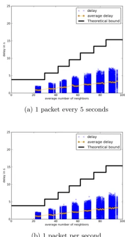
In the remainder of this section, we present the simulation results of RTXP and PEDEMACS with free-space and log-normal shadowing propagation channels. We compare the end-to-end delays of the packets, the energy spent during simulations and the delivery ratio of these protocols. We compare the delays observed during the simulations with the theoretical WCTTs of RTXP and PEDAMACS, respec-tively expressed by Equations 6 and 10. On the figures, the end-to-end delay of a packet is represented by a cross, we choose to represent all the values to be able to observe the distribution of the delays. The circles correspond to the av-erage delay for a given number of neighbors. The black solid curve corresponds to the theoretical WCTT.
6.2.2
Free Space propagation model.
Figures 6(a) and 6(b) respectively represent the end-to-end delay of alarms in function of the average number of neigh-bors for PEDAMACS for 1 packet every 5 second and 1 packet per second rates. First we can notice that all the packets meet their deadlines. This is ensured by the global scheduling. Moreover, the scheduling also ensures that there
(a) 1 packet every 5 seconds
(b) 1 packet per second
Figure 6: PEDAMACS - free-space propagation model
are no interfering nodes communicating at the same time. Since it is the only way to lose a packet with free-space prop-agation model, we observe a delivery ratio of 100%. The de-lay is not affected by the traffic load because the scheduling frame do not change according to it.
Figures 7(a) and 7(b) depict the end-to-end delays and the-oretical bound for RTXP. In this case, we also observe that all the packets meet their deadlines as predicted in Section 5. Moreover, the delivery ratio is also 100%. Nevertheless, the increase in the load affects the delay, it produces an increase of the delay of some packets. This is due to the fact that, when the load increases, it triggers more secondary activ-ity periods because there are more packets which are at the same time in the same interference domain. On the other hand, the delay does not vary with the average number of neighbors.
Energy consumption.
Figure 8 depicts the maximum energy consumption: each point of the curves corresponds to the maximum value for 20 topologies of the same size. The energy calculation for PEDAMACS and RTXP is done respectively according Equa-tions 11 and 8.
(a) 1 packet every 5 seconds
(b) 1 packet per second
Figure 7: RTXP - free-space propagation model
Figure 8: Maximum energy consumption of runtime of PEDAMACS and RTXP
average number of neighbors because the number of nodes increases. Nevertheless, the growth is not very important because the number of hops in the network does not change and the number of packets transmitted remains the same (200 alarms are produced). When the load increases, it does not affect the energy spent by PEDAMACS because the scheduling remains the same.
The energy spent by RTXP grows linearly with the aver-age number of neighbors. This is due to the fact that data packets are broadcasted to the neighbors of the sender. With the 1 packet per second rate, the energy spent is higher than with the 1 packet every 5 seconds rate. The higher the alarm rate is, the more secondary activity periods are triggered. PEDAMACS has a higher energy consumption than RTXP for networks with an average number of neighbors below 50. This is due to the fact that with PEDAMACS the nodes are waking up even if there is no traffic as a result of the scheduling. PEDAMACS is thus more suited to a periodic traffic where all nodes have a packet to send during each scheduling frame than to an alarm traffic. RTXP, on the contrary, adapts to the traffic load. If there is no alarm, nodes sleep most of the time, if there are many alarms, sec-ondary periods are triggered to handle the traffic.
6.2.3
Log-normal shadowing propagation model.
(a) delay
(b) delivery ratio
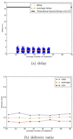
Figure 9: PEDAMACS - log-normal shadowing Figure 9(a) depicts the delay of the packets and the theo-retical bound for PEDAMACS in the case of the log-normal shadowing model. In this case as well, no packet misses its deadline. Nevertheless, Figure 9(b) represents the mini-mum, maximini-mum, and average delivery ratios observed dur-ing the simulations. The values are very low, most of the packets are lost because of the harsh channel conditions. Figure 10(a) depicts the delay of the packets and the
theoret-(a) delay
(b) delivery ratio
Figure 10: RTXP - log-normal shadowing without retransmissions
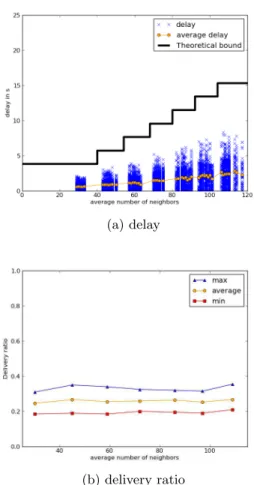
ical bound for RTXP in the case of the log-normal shadowing model with no retransmission mechanism. As in the case of PEDAMACS, all the packets meet the deadline. But, in this case, the delivery ratio (Figure 10(b)) is higher. This is due to the opportunistic scheme implemented by RTXP, which increases the reliability as described in Section 4.4.
PEDAMACS does not implement any retransmission mech-anism. Nevertheless, as described in Section 2.3, the sched-uled protocol LEMMA [24] improves the concept of PEDAMACS by allowing the nodes to access to their transmission slots with a CSMA/CA scheme. It allows the nodes to avoid transient interferences. Moreover, LEMMA also allows to retransmit the data packet several times during a time slot. In order to improve the performances of PEDAMACS, we choose to simulate these LEMMA mechanisms in PEDAMACS time slots. The results can be seen in Figure 11 these ad-ditional schemes improve the delivery ratio of PEDAMACS while allowing to meet the deadline. Nevertheless, the sults are still lower than in the case of RTXP without re-transmission, as can be seen by comparing Figures 11(b) and 10(b): in the case of PEDAMACS, the average is around 65% whereas in the case of RTXP it is around 80%. Figure 12(a) depicts the delay of the packets and the theoret-ical bound for RTXP in the case of the log-normal shadowing model with retransmissions. In this case, we notice that few
(a) delay
(b) delivery ratio
Figure 11: PEDAMACS - log-normal shadowing with LEMMA mechanisms
packets miss the deadline. The retransmission mechanism is described in Section 4.4, if a sender does not detect a jamming code during the Backoff Forward phase, it sends a jamming code in the L slot to trigger a secondary activity period. It then retransmits the packet in the new activity period (in our implementation a packet can be retransmit-ted 5 times per duty cycle, then it is resent in the next duty cycle). In some cases, there are too many retransmissions so the packet cannot meet the deadline. Nevertheless, the retransmission mechanism allows to have a higher delivery ratio even under harsh channel conditions. Figure 9(b) rep-resents the minimum and maximum delivery ratios observed during the simulations. The values are higher than those observed in the case of PEDAMACS even with LEMMA mechanisms and it improves the results of RTXP without retransmissions.
Under harsh radio channel conditions it is not possible to en-sure that all the packets are received. Neither it is possible to ensure that all packets are received before the deadline. This is due to the probabilistic nature of the radio link, in-deed there is a chance that a packet is not correctly received even after many retransmissions. RTXP is designed with the goal of avoiding probabilistic behaviors, channel access and forwarder selection are deterministic, so the behavior is predictable and we can ensure that packets meet their deadline. Nevertheless, the radio channel introduces a
prob-(a) delay
(b) delivery ratio
Figure 12: RTXP - log-normal shadowing with re-transmissions
abilistic aspect, thus one can legitimately ask if it is worth it to have a deterministic protocol on a probabilistic channel. In the next sections this issue is further investigated.
6.3
Comparison with a non real-time solution
In this section, we compare RTXP with a non real-time solu-tion under harsh radio channel condisolu-tions in order to verify that having deterministic behaviors in the protocol actually improves the real-time performance. We choose to com-pare RTXP with a XMAC and gradient routing solution [34]. XMAC [11] is a preamble MAC protocol as described in Section 2.1, but it does not wake up all the neighbors of the sender. The preamble is composed of short packets and response slots. Nodes alternately sleep and wake up. When a node wakes up, it senses the channel, if it receives a preamble packet and is the destination of the packet, it an-swers in a response slot, otherwise it goes back to sleep. In our case, we use an opportunistic gradient routing scheme, meaning that any node that receives a preamble packet and has a smaller hop-count than the sender can answer and be-come the forwarder of the current packet. A node that has a packet to send first senses the channel, if the channel is free it transmits the preamble packets. If it senses activity it backs off for a random duration and retries after. The access to the channel is thus not deterministic.
With the XMAC and gradient protocol, the end-to-end delay depends on the number of hops a packet has to do to reach the sink. A packet has to wait at most for a preamble length to do one hop (at most one duty cycle period). In order to fairly compare this solution with RTXP, we take duty cycle duration of one third of the duty cycle of RTXP (because in RTXP a packet can do up to three hops during a single duty cycle). This choice actually disadvantages RTXP because XMAC preamble lasts half a duty cycle on average. We use Equation 6 as the theoretical bound for XMAC with gradient. XMAC defines an acknowledgment packet and the number of retransmissions can be specified. During the simulations, different values are tested in order to monitor the effect retransmissions have on reliability and delay. The alarm rate used in the simulations is 1 alarm every 5 sec-onds. The channel model is log-normal propagation model. Figures 13, 14 and 15 respectively depict the results for 0, 5 and 500 retransmissions. The same parameters as previously are monitored: end-to-end delay and delivery ratio.
(a) delay
(b) delivery ratio
Figure 13: XMAC with gradient: no retransmission Figure 13(a) shows that every packet, which arrives to the sink, respects the deadline in the case there is no retrans-mission. Nevertheless, the delivery ratio, shown in Figure 13(b), is very low compared to the one achieved with RTXP (as shown in Figure 10(b)).
(a) delay
(b) delivery ratio
Figure 14: XMAC with gradient: 5 retries
shows that some packets miss the deadline. It occurs be-cause the retransmissions increase the end-to-end delay. The delivery ratio, depicted in Figure 14(b) is higher than in the previous case. Nevertheless, the amount of packets that miss the deadline is higher than in the case of RTXP as it can be seen in Figure 12(a). The delivery ratio, represented in Fig-ure 14(b), is higher than in the previous case because packets have more probabilities to be successfully transmitted when the number of retransmissions increases. Nevertheless, the delivery ratio is still smaller than with RTXP as can be seen in Figure 12(b). Moreover the difference between maximum and minimum values of delivery ratio is smaller in the case of RTXP, it is thus more stable.
In our implementation of RTXP, a packet is retransmitted 5 times during one duty cycle. If it still has not be correctly received, it will be retransmitted during the next duty cycle. This means that, in the case of RTXP, there is no bound on the number of times a packet can be retransmitted. Thus, in order to fairly compare RTXP with XMAC gradient, we choose a very high number of retransmissions: 500. As de-picted in Figure 15(a), most of the packets miss the deadline with delays up to several hundreds of seconds. Nevertheless, as shown in Figure 15(b), it results in a slight increase of the delivery ratio, but it remains below the values of RTXP as can be seen in Figure 12(b). These high delays are mostly due to the fact that the high number of retransmissions
in-(a) delay
(b) delivery ratio
Figure 15: XMAC with gradient: 500 retries
duces a high occupation of the channel, resulting in longer delays to access the channel.
These results show that introducing determinism for channel access and routing leads to better performances even with a probabilistic radio link.
7.
CONCLUSION AND FUTURE WORK
In this paper we present RTXP, a solution to handle real-time alarms in WSNs. We describe the proposition and give its theoretical bounds on the end-to-end delay and its real-time capacity. By simulation we compare RTXP and PEDAMACS, a scheduled solution. We show that RTXP is more suited to alarm traffic than PEDAMACS. By simulat-ing the protocols under harsh radio channel conditions, we show that it is not possible to give hard guarantees on the delay under unreliable radio link assumptions. Nevertheless, by favorably comparing RTXP to a non real-time solution, we demonstrate the usefulness of real-time approaches even with unreliable links.
In the future, experimentation on real sensors has to be per-formed in order to verify the performances of our solution. Notably, in reality the assumption of symmetric links may not hold, so we will have to evaluate the capacity of nodes to communicate with jamming codes in these conditions. Nev-ertheless, works such as [10] suggest that jamming codes
so-lution may be more robust to harsh conditions than explicit control packets. In this paper, we derive the theoretical de-lay bound and capacity from general statements made in the protocol description. From these statements, we also con-struct simple proofs of properties of RTXP. Nevertheless, to be trusted, the protocol must be described in a formal lan-guage and verified using a formal verification technique. A future work will thus be to apply model checking techniques to RTXP.
8.
REFERENCES
[1] Cc2500, low-cost low-power 2.4 ghz rf transceiver. [2] http://wsnet.gforge.inria.fr/, viewed 6 march 2013. [3] Ieee standard for local and metropolitan area networks
- part 15.4 : Low-rate wireless personal area networks ( lr-wpans ).
[4] Isa: Wireless systems for industrial automation: Process control and related applications (2009), isa-100.11a-2009.
[5] Rpl: Ipv6 routing protocol for low-power and lossy networks.
[6] I. Amadou. Protocoles de routage sans connaissance du voisinage pour r ˜Al’seaux radio multi-sauts. Phd thesis manuscript, insa de lyon, 2012.
[7] G. Anastasi, M. Conti, and M. Di Francesco. A comprehensive analysis of the mac unreliability problem in ieee 802.15.4 wireless sensor networks. Industrial Informatics, IEEE Transactions on, 7(1):52–65, feb. 2011.
[8] A. Bachir, D. Barthel, M. Heusse, and A. Duda. Micro-frame preamble mac for multihop wireless sensor networks. ICC ’06, pages 3365–3370, Istanbul, Turkey, 2006.
[9] S. Biswas and R. Morris. Exor: opportunistic multi-hop routing for wireless networks. In ACM SIGCOMM Computer Communication Review, volume 35, pages 133–144. ACM, 2005.
[10] C. A. Boano, M. A. Z´uniga, K. Romer, and T. Voigt. Jag: Reliable and predictable wireless agreement under external radio interference. IEEE RTSS, pages 315–326. IEEE, 2012.
[11] M. Buettner, G. V. Yee, E. Anderson, and R. Han. X-mac: A short preamble mac protocol for duty-cycled wireless sensor networks. SenSys ’06, pages 307–320, Boulder, USA, 2006.
[12] M. Caccamo, L. Y. Zhang, L. Sha, and G. Buttazzo. An implicit prioritized access protocol for wireless sensor networks. RTSS ’02, pages 39–48, Austin, USA, 2002.
[13] J. Chen, R. Lin, Y. Li, and Y. Sun. Lqer: A link quality estimation based routing for wireless sensor networks. In Sensors, volume 8, pages 1025–1038, 2008.
[14] J. Chen, P. Zhu, and Z. Qi. Pr-mac: Path-oriented real-time mac protocol for wireless sensor network. ICESS ’07, pages 530–539, Daegu, Korea, 2007. [15] O. Chipara, Z. He, G. Xing, Q. Chen, X. Wang,
C. Lu, J. Stankovic, and T. Abdelzaher. Real-time power-aware routing in sensor networks. IEEE IWQoS 2006, pages 83–92, 2006.
[16] S. Coleri. Pedamacs: Power efficient and delay aware
medium access protocol for sensor networks, ms thesis, electrical engineering and computer science, university of california, berkeley, December 2002.
[17] L. Doherty and K. S. J. Pister. Tsmp: Time
synchronized mesh protocol. DSN ’08, pages 391–398, Orlando, USA, 2008.
[18] C. C. Enz, A. El-Hoiydi, J.-D. Decotignie, and V. Peiris. Wisenet: an ultralow-power wireless sensor network solution. Computer, 37(8):62–70, 2004. [19] S. Ergen and P. Varaiya. Pedamacs: power efficient
and delay aware medium access protocol for sensor networks. In IEEE Transactions on Mobile Computing, volume 5, pages 920–930, 2006. [20] E. Felemban, C. Lee, and E. Ekici. Mmspeed:
Multipath multi-speed protocol for qos guarantee of reliability and timeliness in wireless sensor networks. In IEEE Transactions on Mobile Computing, volume 5, pages 738–754, 2006.
[21] W. R. Heinzelman, A. Chandrakasan, and H. Balakrishnan. Energy-efficient communication protocol for wireless microsensor networks. IEEE HICSS, 2000.
[22] P. Huang, H. Chen, G. Xing, and Y. Tan. Sgf: A state-free gradient-based forwarding protocol for wireless sensor networks. In ACM Trans. Sen. Netw., volume 5, pages 14:1–14:25, 2009.
[23] K. K. Khedo, R. Perseedoss, and A. Mungur. A wireless sensor network air pollution monitoring system. In International Journal of Wireless and Mobile Networks (IJWMN), Vol.2, No.2, pages 31–45, 2010.
[24] M. Macedo, A. Grilo, and M. Nunes. Distributed latency-energy minimization and interference
avoidance in tdma wireless sensor networks. Computer Networks, 53(5):569–582, 2009.
[25] A. Mouradian and I. Aug´e-Blum. 1-d coordinate based on local information for mac and routing issues in wsns. ADHOC-NOW’12, pages 42–55, 2012.
[26] J. Polastre, J. Hill, and D. Culler. Versatile low power media access for wireless sensor networks. SenSys ’04, pages 95–107, Baltimore, USA, 2004.
[27] M. V. Ramesh. Real-time wireless sensor network for landslide detection. In SENSORCOMM ’09, pages 405–409, Athens, Greece, 2009.
[28] U. Roedig, A. Barroso, and C. J. Sreenan. f-mac: A deterministic media access control protocol without time synchronization. EWSN ’06, pages 276–291, Zurich, Switzerland, 2006.
[29] A. Rowe, R. Mangharam, and R. Rajkumar. Rt-link: A time-synchronized link protocol for
energy-constrained multi-hop wireless networks. IEEE SECON, pages 402–411, Reston, USA, 2006.
[30] S. D. Servetto and C. Univerisity. Constrained random walks on random graphs : Routing algorithms for large scale wireless sensor networks. WSNA ’02, pages 12–21, Atlanta, USA, 2002.
[31] J. Stankovic and T. Abdelzaher. Speed: a stateless protocol for real-time communication in sensor networks. ICDCS ’03, pages 46–55, Providence, USA, 2003.
Quality-driven volcanic earthquake detection using wireless sensor networks. RTSS ’10, pages 271–280, San Diego, CA, USA, 2010.
[33] F. Ye, G. Zhong, S. Lu, and L. Zhang. Gradient broadcast: a robust data delivery protocol for large scale sensor networks. Wirel. Netw., 11:285–298, May 2005.
[34] W. Ye, J. Heidemann, and D. Estrin. Medium access control with coordinated adaptive sleeping for wireless sensor networks. In IEEE/ACM Trans. Netw., volume 12, pages 493–506, 2004.
[35] K. Yedavalli and B. Krishnamachari. Enhancement of the ieee 802.15.4 mac protocol for scalable data collection in dense sensor networks. WiOPT’08, pages 152–161, 2008.
[36] M. Zuniga and B. Krishnamachari. Analyzing the transitional region in low power wireless links. SECON ’04, pages 517–526, Santa Clara, USA, 2004.