Relevant Eigen-Subspace of a Graph: A Randomization Test.

HAL Id: hal-00630409

https://hal.archives-ouvertes.fr/hal-00630409

Submitted on 10 Oct 2011

HAL is a multi-disciplinary open access archive for the deposit and dissemination of sci-entific research documents, whether they are pub-lished or not. The documents may come from teaching and research institutions in France or abroad, or from public or private research centers.

L’archive ouverte pluridisciplinaire HAL, est destinée au dépôt et à la diffusion de documents scientifiques de niveau recherche, publiés ou non, émanant des établissements d’enseignement et de recherche français ou étrangers, des laboratoires publics ou privés.

Test.

Alain Lelu

To cite this version:

Alain Lelu. Relevant Eigen-Subspace of a Graph: A Randomization Test.. CAP 2011, May 2011, Chambéry, France. p. 4 à 15. �hal-00630409�

Relevant Eigen-Subspace of a Graph :

A Randomization Test.

LORIA, Nancy - France,

Abstract : Determining the number of relevant dimensions in the eigen-space of a

graph Laplacian matrix is a central issue in many spectral graph-mining applications. We tackle here the sub-problem of finding the “right" dimensionality of Laplacian matrices, especially those often encountered in the domains of social or biological graphs: the ones underlying large, sparse, unoriented and unweighted graphs with a power-law degree distribution. We present here the application of a randomization test to this problem. We validate our approach first on an artificial sparse and power-law type graph, with two intermingled clusters, then on two real-world social graphs (“Football-league”, “Mexican Politician Network”), where the actual, intrinsic dimensions appear to be 11 and 2 respectively ; we illustrate the optimality of the transformed dataspaces both visually, and numerically by means of a decision tree.

Keywords : graph mining, dimensionality reduction, intrinsic dimension, randomization

test, relevant eigen-subspace, graph, graph Laplacian, small-world graph.

1. Introduction

Spectral methods have been recently considered an important approach for extracting knowledge from graphs. For example, spectral graph clustering has been considered by many authors a most promising path to “better” clustering techniques (Von Luxburg, 2007). Or spectral characteristics have been considered relevant clues for finding out “graph motifs” in biological applications (Banerjee, 2008). Not to mention the scientific (and economic...) importance of spectral centrality indices such as PageRank (Brin & Page, 1998) for the study of social networks. Two main questions arise when using graph spectral methods:

What transformation of the dataspace is most relevant for this task? Though the case is far from closed, a consensus exists for considering the dominant eigenspace of one or another of the tightly related “graph Laplacian” matrices as the relevant one.

How many major dimensions must be considered in this transformed dataspace for conveniently observing features or performing graph mining operations? This last problem is the one we try to cope with in the present paper. Many answers have been proposed, mainly in the more general framework of rectangular datatables, but most of them rely on the empirical evidence of a “gap” in the scree-plot of the eigenvalue sequence, whether visual or based on numerical indices such as second differences (Cattell,1966), or on specific statistical models often untrue in the case of large and sparse graphs encountered in most of the social or biological application domains (Bouveyron et al.,2009).

Whereas statistical comparisons with “null models”, i.e. randomized versions of a graph, attract a growing interest for tasks such as graph motifs discovery (Milo et al., 2002), no proposal has been advanced, to our knowledge, on the problem of delimiting by means of a rigorous statistical methodology the relevant eigen-subspace of a graph. We will limit here our investigations to the unoriented and unweighted graphs.

In section 2 we will present a few related contributions. In section 3 we will describe our general TourneBool randomization test and specify it in the case of unoriented and unweighted graphs. In section 4 we will focus on eigenspace approaches in graph studies, and will briefly recall precursor contributions as well as state-of-the-art well-established results. Section 5 will expose the use of the TourneBool test for finding out the relevant eigen-subspace of a graph. Three applications will ensue: in section 6 we will describe our process for generating an artificial 2-cluster sparse graph with a major realistic feature, i.e. a power-law global distribution of the nodes degrees, and the one-dimensional eigen-space resulting from our test. The second and third applications in section 7 involve the well-known “football league” social graph (Girvan & Newman,2002) first, where the TourneBool test delineates an eleven-dimensional relevant eigenspace, visually displaying the main 12-conference loosely intermingled structure as well as the deviations from this structure. A decision tree numerically confirms these nuanced results. And second, the “Mexican politicians network” appears to be strongly structured in a two-dimensional intrinsic embedding. As a conclusion, we will claim that the resultant eigenspace is a stable groundwork for building further representations, whatever data mining method is used.

2. Related approaches

The authors of contribution (Milo et al.,2002) compare an oriented graph to its randomized counterparts (same number of nodes and ingoing/outgoing degree distribution) in order to detect significant directed subgraphs termed “network motifs”. As their objective, far from ours, is mainly focused on detecting elementary building blocks in biological networks, they impose

further constraints on their randomized null models, such as embedding the same repartition of 3-motifs as in the original graph when extracting 4-motifs. The authors of contribution (Banerjee,2008) have other bio-inspired objectives, such as the discovery of motif joinings or duplications when comparing graphs. They show that the full spectra of the graph laplacians, and the resulting spectral plots, include characteristic traces of these events. They explore properties of the whole graph spectra, not properties of null models spectra, or of dominant parts of the spectrum.

In (Lelu & Cadot,2010) we have compared word-text binary matrices to their randomized versions, in order to bring out valid links (and anti-links) in the two inter-texts and inter-words derived graphs. Though tightly related to our present method and tools, none of these approaches deals with the problem of finding out the “right” reduced representation space of a graph. The contribution (Gionis et al., 2007) deals, as we do, with the problem of finding out the number of relevant eigen-dimensions in a rectangular binary matrix, but presents a heuristic approach based on a unique randomized matrix.

3. The Tournebool randomization test

3.1 General case: testing any numerical property for any binary matrix TourneBool (Cadot,2005) is a method for generating random versions of a binary datatable with prescribed margins, and the ensuing test for validating any statistics conducted on it. It is to be noted that the principles of generation of random matrices with prescribed margins seem to have been discovered independently several times, in various application domains: ecology (Connor E & Simberloff, 1979; Cobb & Chen, 2003), psychometrics (Snijders, 2004), combinatorics (Ryser, 1964), sociology (Roberts, 2000). The contribution (Cadot, 2006) legitimates the rigorous permutation algorithm based on rectangular “flip-flops”, and shows that any Boolean matrix can be converted into any other one with the same margins in a finite number of cascading flip-flops, i.e. compositions of elementary rectangular flip-flops: at the crossings of rows i1 and i2, and columns j1 and j2, a rectangular flip-flop keeping the margins unchanged is possible if the (i1,j1) and (i2,j2) values are 1 whereas the (i1,j2) et (i2,j1) values are 0.

As is the case for all other randomization tests (Manly,1997), the general idea comes from the exact Fisher test (Fisher, 1936), but it applies to the variables taken as a whole, and not pairwise. The flip-flops preserve the irreducible background structure of the datatable, but break up the meaningful links specific to a real-life data table. Consider for example a text vs. words incidence matrix: if some words appear in nearly all the texts, they will appear as such in all the simulated matrices too, and no link

between these words will ensue. Now consider a few long texts systematically comprising none of these considered frequent words: the simulated matrices will not reproduce this interesting feature, which will only be brought to light by comparison to the original one. In this way, comparing with simulations allows one to depart the background structural part of a linkage out of the other part, the one we are interested in. The background structure depends on the application domain, and also on the distributions of the margins. For example, most of texts×words datatables have a power-law distribution of the words, and a binomial-like one for the number of unique words in the texts. This background structure induces our “statistical expectation” of no links conditionally to the type of corpus. Getting rid of the background structure enables this method to process any type of binary data, both (1) taking into account the marginal distributions, (2) doing this without any need to specify the statistical models of these distributions.

When using this algorithm, one must fix the values of three parameters: the number of rectangular flip-flops for generating non-biased random matrices, the number of randomized matrices, the alpha risk. The two last parameters are fixed in accordance with the usual compromises: on the computer science side, the trade-off between speed and quality - the more simulated matrices, the higher the quality of estimation, but the longer the computation time, too... For large matrices, we use to ask for 100 or 200 simulations. On the statistical side, the trade-off between the alpha and beta risks: the smaller the alpha value, the lesser the risk of extracting links due to the sole chance, but also the greater the beta risk of rejecting significant and meaningful links. Our experience is to fix the value to the usual 5% or 1%. As for the first parameter (the number of elementary flip-flops), our rule of thumb is to start with four times the number of ones in the matrix, and adjust it, if necessary, considering the sequence of the computed Hamming distances. It is to be noted that the permutation tests, from which emanate the randomization tests, have been proven to be the most “powerful” ones, i.e. to minimize the beta risk for a given alpha risk (Droesbeke & Finne, 1996).

3.2 Application to graphs

As it is, the TourneBool test is akin to be applied to adjacency matrices of bipartite, unoriented, unweighted graphs, as the non-zero elements of such matrices include two symmetric rectangular binary matrices, and this structure is akin to be reproduced when generating random versions as described above. For generating randomized versions of the adjacency matrix of an unoriented, unweighted graph, further constraints have to be imposed at the step of enabling or not a rectangular flip-flop: the square matrix must be kept symmetric and its diagonal empty.

4. Eigen-spaces for graph mining

To the best of our knowledge, the first application of eigen-analysis to graphs dates back to (Benzécri, 1973), when Correspondence Analysis (C.A.) was applied to adjacency matrices. Let us recall that C.A. (Lebart et al., 1984; Greenacre,2007) relies on the eigen-analysis of a matrix Q issued from any two-way correspondence matrix X (in the case of a undirected and unweighted graph, X is binary and symmetric; Q is symmetric, too):

Q = Dr-1/2 X Dc-1/2 (1)

where Dr and Dc are the diagonal matrices of the row and column totals. The eigen-decomposition of Q writes:

Q = U ΛΛΛΛ V’ (2)

where ΛΛΛΛ is the diagonal matrix of the eigenvalues (λ1... λL = 1, L being

the number of connected components; 1 > λL+1 >... > λR > 0, R being the

rank of X). U and V are the eigenvector matrices for the rows and columns respectively. The C.A. factors F and G ensue, by means of products by diagonal matrices:

F = x..1/2 Dr-1/2U ΛΛΛΛ G = x..1/2 Dc-1/2V ΛΛΛΛ (3)

where x.. is the grand total of X. In (Benzécri,1973) Benzécri has shown analytical solutions for simple graphs such as rings or meshes. In (Lebart, 1984) Lebart has generalized to contiguity analysis, and illustrated by showing that the (F2, F3) factor plane representation of the contiguity graph between French counties reconstitutes the appearance of the France map.

An independent research track starting with (Chung,1997) has defined two “normalized graph Laplacians”, namely the symmetric Laplacian (I – Q), where I is the identity matrix, and λ1... λL = 0, L being the number of

connected components; 0< λL+1<...< λR, R being the rank of X, and the

“random walk” variant I - Dr-1 X. Note that the dominant eigenvector of

(Dr-1 X)’ (more precisely of α (Dr-1 X)’ + (1/N)(1- α)11’ for the sake of

“imposing” the presence of one sole connected component) is the PageRank centrality index (Brin & Page, 1998).

Spectral graph clustering consists of grouping the nodes in a K-dimensional major eigen-subspace – for a review see (Von Luxburg, 2007) – and is an increasingly active research line. To our knowledge and up to now, the problem of determining the number K, when the distribution of degrees is non-Gaussian, has not received more satisfactory answers than the scree-plot visual or second-difference heuristics (Cattell,1966), visually prominent in the case of small graphs, but difficult to put into practice in the case of large ones.

5. Determining the relevant eigen-subspace of a graph with Tournebool A well-established result in data analysis states that the relevant, noise-filtered information lies in the dominant eigen-elements of a data matrix

(Chung, 1997). In the case of the Q matrix, Benzécri, Chung and many others have shown that the value of its first eigenvalue, of multiplicity L (L being the number of connected components), is one. The same is true of the Dr-1 X matrix the representation space of which seems to be preferred by

many authors. Thus our test sets apart the case of this dominant eigenvalue, of value one in the randomized versions of Q or Dr-1 X too, and answers to

the sequence of questions: does the (L+1)th, (L+2)th, ... eigenvalues significantly exceed their randomized equivalents ? Our test then writes:

• Generate a sufficient sample (X1, X2, ... Xp) of randomized versions of the original matrix X0 (e.g. 200 matrices).

• Extract the full sequence of singular values of Q0 or Dr-1 _{X0, in}

decreasing order.

• For each k-order eigen-space, starting from k = L+1, compare the k-th

singular value of Q0 or Dr-1 X0 to the set of corresponding k-th singular

values in the sample: if the current singular value λk is greater than or equal to the randomized one located at the significance threshold (e.g. than the third one at the 99% threshold, here), it is deemed significantly diverging from randomness, and the algorithm goes on with k = k + 1.

When the algorithm stops, the value k-L-1 is the dimension number of the relevant eigenspace.

6. Validation: artificial graph adjacency matrix

We will focus on trying to reproduce two characteristics that stand out from the general experience of real-world social or biological graphs: 1) a power-law distribution of their degrees; 2) cluster structures which are by no way all-or-none phenomena: they rather amount to progressive, fuzzy memberships around dense data-cores. In other words, clusters are generally intricate, entangled, and by no way orthogonal.

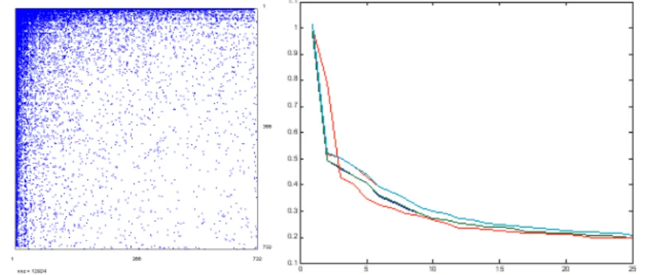
Figure 2 – At left: The two-cluster M0 random adjacency matrix with minimum degree 4, and a

power-law degree distribution. At right: The “scree-plot” of the 50 first eigenvalues derived from

M0 (solid red line) compared to the variation intervals of its randomized counterparts. By

6.1 Data generation:

We will first build such intertwined clusters in the simplest case of two clusters, by generating a one-cluster table, e.g. appending a full (750, 800) “ones" matrix and a full (750, 660) “zeros" one, then creating another (750, 1460) matrix by randomly permuting the columns, and eventually stacking the two matrices into a (1500, 1466) one. The second step consists in “morphing" this matrix so as to fit to some prescribed relative column and row sum profiles (e.g. a power-law distribution for the column sums, and a binomial one for the row sums): the process of alternating a global stretching or expanding for each column vector so as to fit to the corresponding prescribed sum profile, then doing the same for the row vectors, lets the transformed datatable converge to a real positive matrix embedding a (distorted) memory of the initial structure. The third step consists in turning this table binary, first by normalizing it (i.e. dividing by its maximum value), then by considering each value proportional to a probability for drawing a value “one”; the resulting (1500, 1460) table comprises many empty columns, or columns summing to 1 or 2; in a final cleansing process, we remove these columns in order to prevent side effects, and we now yield a (1500, 836) binary matrix X0 with a power-law distribution of the column sums. The last phase consists in building a symmetric power-law binary adjacency matrix starting from the symmetric (836, 836) matrix Z0 = X0’ X0, on the same principles: morphing and pruning Z0 into a symmetric power-law real matrix with an empty diagonal, then “binarize” it by means of the above-described probabilistic process.

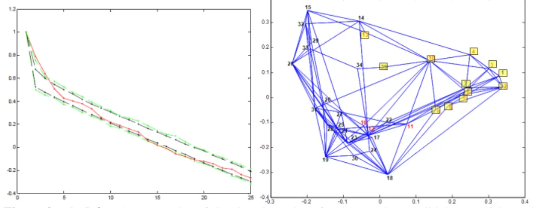
Figure 3 – At left: The 2-cluster intertwined structure in matrix M0, highlighted by sorting the

rows and columns along the U2 values. At right: The 828 nodes in the (U2, U3) plane.

The final result is a M0 (828, 828) adjacency matrix with minimum degree 4 (see Figure 2, left) and a power-law degree distribution.

6.2 Results

Eigenspace test: Figure 2 (right) shows the “scree-plot” of the 50 first eigenvalues of Q0, compared to the plot of the 99% confidence interval of its 200 randomized counterparts generated by Tournebool. As jumps out

from the figure, the only “first” (i.e. second) singular value dominates their confidence intervals, emphasizing the 2-cluster intertwined structure, visually evident when sorting the rows and columns along the U2 values (figure 3, left).

7. RELEVANT EIGEN-SUBSPACE OF REAL-WORLD SOCIAL

GRAPHS

7.1 The Football-league graph

The graph of the regular-season Division I college football game for the year 2000 (GIRVAN & NEWMAN, 2002) is an interesting small real-life test

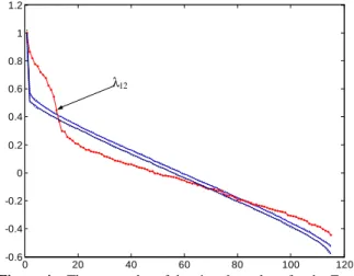
social network in that it includes the “theoretical” social structure made of 12 regional “conferences”, in addition to the unsupervised structure emanating from the 115-node graph. The TourneBool test with 200 randomized adjacency matrices, at the 99% confidence threshold results in the scree-plot shown in Figure 4: the eleven “first” eigenvalues (N°2 to N°12, as there is a single connected component in the graph) of the original Dr-1 M0 matrix clearly dominate the confidence “corridor” of its 200

randomized counterparts. 0 20 40 60 80 100 120 -0.6 -0.4 -0.2 0 0.2 0.4 0.6 0.8 1 1.2 λ12

Figure 4 – The scree-plot of the singular values for the Football-league social graph (solid line in

red). The dotted lines delimit the 99% confidence interval, the solid blue ones delimit the minimum to

maximum observed variation interval. By construction, the first eigenvalue of any diag(d°)-1 M

stochastic matrix is 1.

Figures 5 and 6 display the (U2, U3) and (U11, U12) planes in which conferences appear with different colors. Eye-catching evidence in these example plots show that all-or-none clustering results, as well as nuanced remarks about deviations out of the theoretical structure, depending on the conference, may be pulled out from this representation. In contrast, the U13

to U15 factors display no outstanding evidence of interpretable structures. An important remark is that this dataspace “normalizes” the group phenomena, whatever the number of concerned individuals: small striking phenomena are highlighted in the same way as large trends.

Factor 2 and Factor 3

-0,2 -0,15 -0,1 -0,05 0 0,05 0,1 0,15 0,2 0,25 -0,2 -0,15 -0,1 -0,05 0 0,05 0,1 0,15 Atlantic Coast Big East Big Ten Big Twelve Conference USA Independents Mid-American Mountain West Pacific Ten Southeastern Sun Belt Western Athletic

Figure 5. The (U2, U3) plane. Each conference has its own color, and a line with this color connects its teams, from the first one to the last one.

Factor 11 and Factor 12

-0,2 -0,1 0 0,1 0,2 0,3 0,4 0,5 -0,2 -0,1 0 0,1 0,2 0,3 0,4 0,5 Atlantic Coast Big East Big Ten Big Twelve Conference USA Independents Mid-American Mountain West Pacific Ten Southeastern Sun Belt Western Athletic

Figure 6 – The (U11, U12) plane. Each conference has its own color, and a line with this color

connects its teams, from the first one to the last one.

We have quantitatively tested this remark, performing a grid-optimized decision tree in the 11-dimensional eigen-subspace: Table 1 shows which conferences may be accurately, if not perfectly, reconstructed, starting from the eigen-subspace, and which may not (e.g. the “Independents” or “Sun Belt” conferences).

TABLE I. RULES ISSUED FROM A DECISION TREE IN THE 11-D RELEVANT

EIGEN-SUBSPACE U2:U12 FOR RECONSTITUTING THE 12

FOOTBALL-CONFERENCES (T,TP,FP stand for True, True Positive, True Negative respectively).

Conferences Rules Number of

T TP FP F-score 0-Atlantic Coast 1-Big East 2-Big Ten 3-Big Twelve 4-Conference USA 5-Independents 6-Mid-American 7-Mountain West 8-Pacific Ten 9-Southeastern 10-Sun Belt 11-Western Athletic U5<-0.146 U10<-0.136 U6>0.1 & U3>0.05 U4>0.115

U7<-0.1 & U10>0.1 U11<-0,01& U12>0.12 U2>0.05 & U3>0.1 U9>0.16

U2<-0.132 U3<-0.131 3.U11+2.U12>0.7 U6>0.06 & U7<-0,1

9 8 11 12 10 5 13 8 10 12 7 10 9 8 11 12 9 2 13 8 10 12 7 8 0 0 0 0 0 0 0 0 0 0 3 1 1 1 1 1 0.95 0.57 1 1 1 1 0,82 0,84

7.2 The Mexican politicians network

The social graph « Mexican Politician Network »

(http://vlado.fmf.uni-lj.si/pub/networks/data/esna/Mexican.htm) linking 35 Mexican politicians at

the end of the 20th century, has been studied by (de Nooy et al.,2004) and is available online. Some of them are belong to the army: it is interesting to investigate whether this belonging is, or is not, a structuring feature of the global network of the political power in this country.

Figure 9 – At left: The scree-plot of the singular values for the Mexican politicians social graph

(solid line in red). The black dotted lines delimit the 99% confidence interval; the pale green ones delimit the minimum to maximum observed variation interval. At right: The (U2, U3) plane. In red: Army officers; Boxes: a decision tree solution maximizing the Augmented Rand Index when comparing to the Army/civilian partitioning.

Figure 9 (left) ensues from the TourneBool test, at the confidence threshold of 99%, on 2000 randomized adjacency matrices: the two « major »

eigenvalues (N°2 and N°3, as this graph comprises a unique connected component) of the Q = D-1/2 M0 D-1/2 matrix are clearly dominating the « confidence corridor » issued from the 2000 corresponding matrices. Figure 9 (right) shows the projection of the 35 politicians in the (U2, U3) plane which constitutes the entire intrinsic space of this graph. Army officers appear in red: a three-pole organization appears visually, one pole is dense, mainly including army officers, except two (central) civilian politicians (F. Madero, E. Portes Gil), and the two others mainly comprise civilians.

8. Conclusions, perspectives

We have shown that the TourneBool randomization test succeeded in finding out the most relevant reduced dataspace for graphs of known structure: an artificially generated 828 nodes graph endowed with a 2-cluster structure and a power-law degree distribution gave rise to a one-dimensional relevant eigen-subspace; the real-life example of “Football league” social network with 12 categories gave rise to an eleven-dimensional relevant eigen-subspace. Another social graph (“Mexican politicians”) with three structuring poles gave rise to a two-dimensional relevant eigen-subspace.

Having a robust estimate of the “right dimensionality” of a graph opens many perspectives:

• It provides a lower bound for the “real number” of possible clusters, which is a precious help for many graph clustering methods.

• It gives a stable base for deriving the “best possible reconstitution” of the adjacency matrix, in order to identify fortuitous links akin to be filtered and potential links particularly consistent with the logics at work in the studied network - a useful feature for recommender systems.

It opens the way to coping with other long-time pending problems, such as: are there real distinct clusters in large, Zipfian graphs, or progressive gradients, or multi-scale structures, or a mix of these elements? How many of them, in what proportions? Our current research line is dealing with these yet unsolved problems.

References

BANERJEE, J. (2008). On the spectrum of the normalized graph Laplacian.

Linear Algebra and its. Applications, 428, p. 3015-3022.

BENZECRI J.-P.(1973). L'analyse des données (3 tomes). Dunod.

BOUVEYRON C., CELEUX G. and GIRARD S. (2009): Intrinsic Dimension

Estimation by Maximum Likelihood in Probabil. PCA. Preprint, in: HAL n°00440372.

BRIN S. & Page L. (1998). The PageRank hypertextual Web Search Engine.

CADOT M. (2005). A simulation technique for extracting robust association rules. In:CSDA 2005, Chania, Greece

CADOT M. (2006). Extraire et valider les relations complexes en sciences

humaines : statistiques, motifs et règles d’association. PhD. thesis, Université de Franche-Comté.

CATTELL R.B. (1966). The scree test for the number of factors. Multivariate

Behavioral Research. 1(2), p. 245-276.

CHUNG F.R.K. (1997). Spectral Graph Theory. CBMS Regional Conference

Series in Mathematics, No. 92, American Mathematical Society.

COBB G.&CHEN Y. (2003). An application of markov chain monte carlo to

community ecology. The American Mathematical Monthly. p. 264–288. CONNOR E&SIMBERLOFF D. (1979). The assembly of species communities: Chance or competition? Ecology. p. 1132–1140.

DE NOOY W.,MRVAR A.,BATAGELJ V.(2004). Exploratory Social Network

Analysis with Pajek. Cambridge: Cambridge University Press.

DROESBEKE J & FINNE J. (1996) Inférence non-paramétrique – Les

statistiques de rangs. Editions de l’Université de Bruxelles.

FISHER R. (1936). The use of multiple measurements in taxonomic problems. Annals of Eugenics p. 179–188.

GIONIS A., MANNILA H., MIELIKÄINEN T., TSAPARAS P. (2007). Assessing

data mining results via swap randomization. ACM Trans. Knowl. Discov.

Data.

GIRVAN M.&NEWMAN M.E. J. (2002). Community structure in social and biological networks. Proc. Natl. Acad. Sci. USA 99, p. 7821–7826.

GREENACRE M. (2007). Correspondence Analysis In Practice. Chapman &

Hall/crc Interdisciplinary Statistics Series.

LEBART L., MORINEAU A., WARWICK K. (1984). Multivariate Descriptive

Statistical Analysis. John Wiley and sons, New-York

LEBART L. (1984). Correspondence Analysis of Graph Structure - Inv. Comm. Meeting of the Psychometric Society (Jouy-en-Josas), Bulletin

Technique du CESIA, vol 2, p. 5-19.

LELU A.&CADOT M(2010). Statistically valid links and anti-links between

words and between documents. Advances in Knowledge Discovery and

Management (AKDM), Springer, p. 307-324.

MANLY B. (1997). Randomization, Bootstrap and Monte Carlo methods in

Biology. Chapman and Hall/CRC.

MILO, SHEN-ORR, ITZKOVITZ, KASHTAN, CHKLOVSKII, AND ALON (2002). Network Motifs: Simple Building Blocks of Complex Networks. Science vol. 298, p. 824-827.

ROBERTS J. M. (2000). Simple methods for simulating sociomatrices with

given marginal totals. Social Networks. Vol. 22, pp. 273-283. RYSER H. (1964). Recent Advances in Matrix Theory. Madison.

SNIJDERS T. (2004). Enumeration and simulation methods for 0-1 matrices with given marginals. Psychometrika. p. 397–417.

VON LUXBURG L., A. (2007). Tutorial on Spectral Clustering. CoRR