aliFreeScan: une approche sans alignement pour annoter l’ARN non codant dans des données génomiques à l'aide d'apprentissage machine

(1)

ALIFREESCAN: UNE APPROCHE SANS ALIGNEMENT

POUR ANNOTER L’ARN NON CODANT DANS DES

DONNÉES GÉNOMIQUES À L’AIDE

D’APPRENTISSAGE MACHINE

par

Ali Fotouhi

Mémoire présenté au Département d’informatique

en vue de l’obtention du grade de maître ès sciences (M.Sc.)

FACULTÉ DES SCIENCES

UNIVERSITÉ DE SHERBROOKE

Sherbrooke, Québec, Canada, April 16, 2020

(2)

Le April 16, 2020

Le jury a accepté le mémoire de Ali Fotouhi dans sa version ﬁnale

Membres du jury

Professeur Shengrui Wang Directeur

Département d’Informatique Professeur Aïda Ouangraoua

Codirectrice

Département d’Informatique Professeur Djemel Ziou

Membre interne Département d’Informatique

Professeur Manuel Lafond Président-rapporteur Département d’Informatique

(3)

Sommaire

Dans ce mémoire, nous essayons de trouver un moyen d’annoter le génome en exploitant uniquement les informations de séquence pour toute famille d’ARN. Nous avons évalué le potentiel des approches d’apprentissage automatique pour l’identification du génome entier des ARN non codants (ARNnc). Nous avons testé plusieurs al-gorithmes et identifié plusieurs défis pour développer une méthode d’apprentissage automatique précise pour la recherche d’ARNc dans les génomes. L’annotation du génome est l’identification d’éléments de séquence fonctionnels dans le génome d’un organisme. La connaissance de la présence et de la localisation de ces éléments de séquence, associée à la compréhension de leurs rôles fonctionnels, aide à révéler le type de processus biologiques qui se déroulent dans l’organisme ainsi que l’historique de son évolution. Les classes d’éléments de séquence fonctionnels comprennent les gènes codant pour les protéines, les éléments d’ARN non codants, ainsi que d’autres. Les éléments d’ARN fonctionnels sont des ARN qui ne sont pas traduits en pro-téines, mais remplissent plutôt leur fonction biologique directement en tant qu’ARN. L’annotation des ARN est généralement effectuée à l’aide d’ARN connus en tant que requêtes pour des recherches d’homologie avec le génome entier étudié. Nous présen-tons les résultats de l’analyse du génome en utilisant uniquement les informations de séquence des ARN sous forme de requêtes de prédiction.

Mots-clés: Annotation du génome; ARN-non-codants; Techniques d’apprentissage.

(4)

Summary

In this thesis, we try to find a way to annotate the Genome exploiting only the sequence information for any RNA family. We have evaluated the potential of machine learning approaches for whole-genome identification of non-coding RNAs (ncRNAs). We have tested several algorithms and identified several challenges to developing an accurate machine learning method for the search of ncRNAs in genomes. The Genome annotation is the identification of functional elements of the sequence in the genome of an organism. Knowledge of the presence and location of these sequence elements, combined with an understanding of their functional roles, helps to reveal the type of biological processes that take place in the organism as well as the history of its evolution. The classes of these elements include protein-coding genes, non-coding RNA (ncRNA) elements, and others. ncRNAs are RNAs that are not translated into proteins, but rather fulfill their biological function directly as RNA. RNA annotation is typically performed using known RNAs as queries for homology searches against the entire genome being studied. We present the results of the genome analysis using only the RNA sequence information as queries for the prediction of ncRNAs.

(5)

Remerciements

Dans la voie de la réussite de mon mémoire, j’ai obtenu l’aide de nombreuses personnes et je veux proﬁter de cette occasion pour remercier tous ceux et celles qui m’ont aidé en cours de route pour atteindre cet objectif. En particulier, je suis re-connaissant pour mes conseillers de recherche, les professeurs Shengrui Wang et Aïda Ouangraoua pour leurs conseils et leur soutien continu tout au long de mon mémoire. Leur patience et leurs connaissances ont été précieuses tout au long de ma recherche, et je leur exprime ma profonde gratitude pour m’avoir donné l’opportunité de par-ticiper à cette recherche. Je suis redevable à mes parents de toujours m’encourager et de se tenir à mes côtés. Je tiens à remercier ma meilleure amie, ma chère Mina Majidi, pour ses encouragements sans ﬁn et son soutien mental à tout moment et en tout lieu.

(6)

Abbreviations

CM Covariance Model

ncRNA non-coding Ribonucleic acid mRNA Messenger Ribonucleic acid ML Machine Learning

MML Multimodal Machine Learning wl Window Length

MWL Multiple Window Length SWL Single Window Length sz Shift Size

seq Sequence seg Segment

NOS Number of Segments rc Reverse Complement

(7)

List of Figures

2.1 Sliding window approach for segment extraction.. . . 10

2.2 Average length of sequences for families in training data. . . 12

2.3 Frequency of the sequence lengths of all families in the training data. 13

2.4 Average length of embedded RNA sequences in the genome. . . 14

2.5 Frequency of the embedded RNA sequences’ lengths in the genome. . 15

(10)

List of Tables

2.1 Confusion matrix. . . 18

2.2 Overall view of the used methods and their results. . . 19

3.1 10-fold cross validation - Method1. . . 22

3.2 Evaluation of the classiﬁers on test/unseen data - Method1. . . 22

3.3 Classiﬁer result - Method1.. . . 23

3.4 Behaviour of Method1 in diﬀerent window lengths for tRNA and Ham-merhead_3. . . 24

3.6 Evaluation of the classiﬁers - Method2. . . 26

3.7 Classiﬁer result including tRNA and noise. . . 27

3.8 Classiﬁer result including U5 and noise. . . 27

3.9 Classiﬁer result including MIR159 and noise. . . 28

3.10 Classiﬁer result including tmRNA and noise. . . 28

3.13 Classiﬁer result - Method4. . . 34

3.14 Classiﬁer result - Method4 with rc. . . 34

3.15 Predicted label for some of the sequences using Method4. . . 35

3.16 Top frequent patterns in all sequences. . . 36

3.17 Top frequent patterns per family. . . 36

3.18 Number of frequent patterns from each k − mer.. . . 39

3.19 Quantity of common frequent patterns occurrences in families. . . 39

(11)

List of Tables

3.22 Classiﬁer report - Method5 reduced features. . . 41

3.23 Classiﬁer report - Method5 reduced features with rc. . . 41

3.26 Classiﬁer report - 5-6-7mers. . . 43

3.27 Classiﬁer report - 5-6-7mers - rc . . . 43

A.1 Information about RNA Families in training data. . . 48

A.2 Information on bucketing the RNA families based on the length (wl intervals). . . 51

A.3 Comparison between number of sequences and their generated seg-ments - Method4. . . 54

(12)

Chapter 1 Introduction

In this chapter, we start with presenting some background information and the description of the problem studied in this thesis. Then we specify the objective of this thesis.

1.1 Background

The central dogma of molecular biology states that gene sequences (DNA) are transcribed into RNA according to the law of chemistry and physics. Ribonucleic Acids (RNAs) are transcripts of portions of DNA called genes. In DNA, every gene consists of two complementary nucleotide strands that are coupled through A-U and G-C bonds that ﬁt in a helix. After transcription, RNA is composed of a single strand of nucleotides that can fold back on itself in various structures, called secondary structures. There are two types of RNA: coding RNAs, which are translated into proteins, and non-coding RNAs (ncRNAs), which realize multiple functions such as functional RNAs. The function of these RNAs is intrinsically linked to their folding structures [8, 1].

Non-coding RNAs are involved in translation, splicing, gene regulation, and other functions [23]. Several well-known ncRNAs such as transfer RNAs or ribosomal RNAs can be found throughout the tree of life. They fulﬁll central functions in the cell and

(13)

1.2. Literature Review

thus have been studied for a long time [34]. Many non-coding RNAs (ncRNAs) are short (often, 100 nucleotides [nt] or less) [16], they are poorly conserved at the sequence level, and may vary dramatically in length.

The assumption that RNA can be readily classified into either protein-coding or non-protein–coding categories has pervaded biology for close to 50 years. Until re-cently, discrimination between these two categories was relatively straightforward: most transcripts were clearly identifiable as protein-coding messenger RNAs (mR-NAs), and readily distinguished from the small number of well-characterized non-protein–coding RNAs (ncRNAs). Well-known types (family) of non-coding RNAs include transfer (tRNAs) and ribosomal RNAs (rRNAs). Recent genome-wide stud-ies have revealed the existence of thousands of non-coding transcripts, whose function and significance are being discovered but still incomplete [6].

Many different types of functional non-coding RNAs participate in a wide range of important cellular functions but the large majority of these RNAs have not been annotated in published genomes. The transcription of a subset of genes into comple-mentary RNA molecules specifies a cell’s identity and regulates the biological activi-ties within the cell. Collectively defined as the transcriptome, these RNA molecules are essential for interpreting the functional elements of the genome and understanding development and disease [19]. So identifying these RNAs and annotating them are crucial tasks.

Several programs have been developed for RNA identification, including specific tools tailored to a particular RNA family as well as more general ones designed to work for any family. Many of these tools utilize covariance models (CMs), statistical models of the conserved sequence, and the structure of an RNA family [26]. We briefly discuss the idea of genome annotation and some of the existing tools.

1.2 Literature Review

1.2.1 Genome annotation of ncRNAs

It has been demonstrated in numerous studies that the true catalog of RNAs encoded within the genome (the "transcriptome") is more extensive and complex

(14)

than previously thought [13, 18]. However, mRNAs account for only 2.3% of the human genome [13], and therefore the vast majority of this unexpected transcription, sometimes referred to as "dark matter" [12, 31], appears to be non–coding. The implicit challenge that this matter presents to our understanding of the expression and regulation of genetic information called for new techniques for the discovery of these ncRNAs.

Unsurprisingly, a great deal of attention is now focused on the non-coding tran-scriptome, leading to the discovery of thousands of small RNAs (<200 nt in length). Many of these have since been classiﬁed into novel categories on the basis of function, length, and structural/sequence features [11].

Genome annotation is the identiﬁcation of functional sequence elements in an organism’s genome. Functional ncRNA elements are RNAs that are not translated into proteins, but rather carry out their biological function directly as RNAs. Much like proteins, many of these RNAs fold into a speciﬁc three-dimensional structure that is intrinsically related to their function. Knowledge of the presence and location of these sequence elements coupled with the understanding of their functional roles help reveal the type of biological processes that take place in the organism as well as the evolutionary relationships between organisms. Classes of functional sequence elements include protein-coding genes, non-coding RNA elements, as well as others [26].

RNA annotation is typically performed using known RNAs as queries for ho-mology1

searches against the entire genome being studied. Despite the widespread importance of functional RNAs, the large majority of them have not been annotated in published genomes [26]. RNA annotation could be a tedious task for several rea-sons: as mentioned earlier RNAs tend to be short and search is carried out at the RNA/DNA level, which may have lower statistical power due to the smaller alphabet size [26]. The size of the genomes being searched also calls for eﬃcient algorithms able to process large sequence databases in a reasonable time.

To cope with the reduced statistical signal, the most successful RNA homology search programs take advantage of the structural conservation of many functional

1. Homology is a concept that takes into account similarities that occur among nucleic acid sequences.

(15)

RNAs by scoring a combination of the conserved sequence and the secondary structure of an RNA family [12]. Sequence- and structure-based tools can be divided into two categories:(1)these that are speciﬁc tools designed for a particular RNA family; and (2) general tools that can work for any family.

1.2.2 Previous studies

The most widely used RNA homology search tool targets the single largest gene family, tRNAs. The tRNAscan-SE program [24, 5] uses a powerful statistical model called the covariance model (CM) that scores candidates based on both their sequence and predicted secondary structures. Covariance models (CMs) are probabilistic mod-els of sequences and secondary structures of an RNA family [10,8].

CMs are constructed from multiple sequence alignments of known homologs of the family that are annotated with a consensus secondary structure. A CM is use-ful for creating sequence- and structure-based multiple sequence alignment of those homologs. CMs are analogous to profile hidden Markov models, commonly used for linear sequence analysis of protein domain families, but with added complexity for modeling a conserved secondary structure. Like CMs, a profile HMM is constructed from an alignment of homologous sequences (but without structure annotation) [26]. CMs, which are shown to be slow, outperform sequence-based methods particu-larly well for families like tRNA that are short (about 70 nucleotides) and exhibit low levels of sequence similarity while maintaining a highly conserved secondary struc-ture. To deal with the slow search speed of CMs, tRNAscan-SE uses tRNA-specific prefilters that allow to ignore a large fraction of the database, leaving only promising subsequences to be evaluated by the slow CM methods. The result is a tool fast enough to search large mammalian genomes on a desktop computer in a few hours [26].

The strategy of using fast family-specific filters before a CM-based search is em-ployed by other family-specific RNA search tools as well. For example, the Bcheck program [36] uses the sequence and structure-based pattern matching program RN-ABOB [9] as a fast prefilter for CMs to identify RNase-P genes. RNABOB, like other pattern-matching programs, identifies subsequences that can fold into a particular

(16)

structure based on user-deﬁned constraints. SRPscan [30] uses the same strategy to identify the signal recognition particle RNAs (SRP RNAs). Due to the higher com-plexity of their algorithms, CMs may be impractical when searching large sequence databases but still, they are more sensitive (able to ﬁnd more true homologs) than sequence-only-based searches [26].

There are some other sequence- and structure-based tools such as Aragorn [21] that do not use CMs. Aragorn is a tRNA and tmRNA finder that uses a tRNA-specific search algorithm for searching the part of a highly conserved B-box consensus sequence as an alignment around that seed. Aragorn’s sensitivity is similar to tRNA-SE but faster. The Arwen [22] is another program from the developers of Aragorn which works in a similar way to detect tRNA genes in metazoan mitochondrial nu-cleotide sequences. Therefore, these methods produce the same results using different methods than CM and are slightly faster.

Structure-based methods are not necessary for all RNAs. For longer RNAs (about 1500nt) sequence-based homology search methods perform well due to a high level of sequence conservation [26]. They are sometimes annotated using the pairwise sequence similarity search tool BLASTN [3] with homologous query sequence from closely related species, or with the RNAmmer tool [20] based on sequence-based proﬁle hidden Markov models.

With the exception of tRNAscan-SE, not many of these tools are commonly used for annotating a genome. Genomes are usually annotated using the Infernal software package. Infernal[28, 27, 26] is one of the most used tools for annotating genomes. Infernal is a software package that implements general CM search methods that can be used for any RNA family. It includes programs to build a CM from an alignment, search a target sequence database with a CM, and create multiple sequence alignments of putative homologs with a CM.

All existing homology search methods rely on alignment techniques, which makes them time-consuming. They also use both sequence and secondary structure infor-mation of RNAs. CMs are more sensitive than sequence-only-based searches but are much slower due to the higher complexity of their scoring alignment algorithms to the point of being impractical when searching large sequence databases. An alternative way for these methods is Machine learning models.

(17)

1.2.3 Machine learning relevance to genome annotation

Originally a branch of artiﬁcial intelligence, machine learning has been fruitfully applied to a variety of domains. The basic idea of machine learning (in our case speciﬁcally supervised learning) is to construct a mathematical model for a particular concept (an element class in the case of genome annotation) based on its features in some observed data. The model can then be applied to identify new instances of the concept in other data [25, 2,35].

One major reason for the popularity of machine learning methods is their ability to automatically identify patterns in data. This is particularly important when the expert knowledge is incomplete or inaccurate, when the amount of available data is too large to be handled manually, or when there are exceptions to the general cases. Machine learning methods are also good at integrating multiple, heteroge-neous features. This property allows the methods to detect subtle interactions and redundancies among features, as well as to average out random noise and errors in individual features. Another strength of machine learning is its ability to construct highly complex models needed by some genomic element classes [35].

Three aspects of data integration by machine learning deserve more discussions. First, the input features could contain redundant information. Different machine learning methods handle redundant features in drastically different ways [17, 7]. Sec-ond, if a large number of features are integrated but the amount of training examples is limited (a phenomenon quite common in genome annotation), multiple issues could come up. The training examples may not be sufficient to capture the combination of feature values characteristic of the classes to be modeled. Third, it could be difficult to combine features of different data types [35], i.e. RNA primary and secondary structures’ information.

An ultimate goal of genome annotation is to identify all types of functional ele-ments and all their occurrences in a genome. However, classifying these novel RNA species remains a challenging task, and we have merely only a vague idea of what subcategories exist, and how we might use experimental or sequence information to distinguish between them. Currently, there are still likely undiscovered genomic ele-ment classes given the rapid discovery of new classes (such as many non-coding RNAs) in recent years. Some element classes also have so far very few discovered instances.

(18)

1.3. The purpose of this thesis

Indeed, the RNA world does not seem to have unveiled all its secrets [33].

In terms of machine learning, these two facts imply that currently, it is impossible to perform purely supervised learning for all element classes2

. Using this terminology, we use the machine learning approach to explore the genomic data.

1.3 The purpose of this thesis

As discussed earlier, CMs outperform sequence-based methods, particularly for short families. Interestingly, however, long ncRNAs (>200 nt) appear to comprise the largest portion of the mammalian non-coding transcriptome. The biological sig-niﬁcance of these long ncRNAs is controversial. Despite an increasing number of long ncRNAs having been shown to fulﬁll a diverse range of regulatory roles, the func-tions of the vast majority remain unknown and untested. This is also true of small RNAs to some extent. Nevertheless, there is an ongoing lack of clarity regarding the true number of ncRNAs within the genome. We expect that detection of ncRNAs throughout the genome could exploit a novel machine learning technique.

There are several challenges in applying machine learning techniques to genome annotation and the corresponding key research problems like lack of training examples and unbalanced positive and negative sets. For some classes of genomic elements, there are insuﬃcient known examples for supervised machine learning methods to capture the general patterns of the classes. With the spread of high-throughput DNA sequencing, each day more RNA-seq data is being produced rapidly, which may pave the way for emergence and development of automated methods to exploit these large volumes of sequence data.

By its very nature, genomics produces large, high-dimensional data sets that are well suited to analysis by machine learning approaches. We have evaluated the poten-tial of machine learning models for whole-genome identification of non-coding RNAs (ncRNAs). We have tested several algorithms and identified several challenges to de-veloping an accurate machine learning method for the search of ncRNAs in genomes. In this thesis, we try to find a way to annotate the genome exploiting only the se-quence information for any RNA family. We discuss RNA annotation in the genome,

(19)

1.3. The purpose of this thesis

highlighting challenges speciﬁc to RNA sequences using Machine Learning techniques. We present the results of the scanning genome utilizing just the sequence informa-tion of the RNAs as queries for predicinforma-tion. In the basic setting, the framework is constructed from observed examples with known labels (RNAs), which is called the supervised learning setting. Then using these examples as queries we would be able to scan the entire genome looking for ncRNAs.

The rest of the thesis is organized as follows. In Chapter2we define the data that will be used and the underlying challenges. In Chapter3 we propose our approaches to tackle this problem. Different methods are used as part of each approach. These methods are chosen based on the defined challenges and we aim to eliminate them step by step. We also interpret the results for each method which directs us to the next method. Finally, we conclude with remaining challenges and the perspective to be considered.

(20)

Chapter 2 Experimental Framework

In this chapter, we provide information about the applied ML models, the data acquisition process, and its characteristics. The initial challenges are discussed as well. Finally, we summarize the methods discussed in this study.

2.1 Challenges

Our goal is to identify the functional elements and occurrences of ncRNAs through the genome applying different Machine Learning models. This concept (ncRNA iden-tification) falls under supervised learning. Our ML approach is constructed from observed examples (ncRNA sequences and noise) with their labels (family name). We scan the genome using the sliding window approach, extracting segments and then the trained model is used to predict the label of these segments categorizing them in different RNA families. Figure2.1 depicts the sliding window approach with a window length of 20 (wl = 20) and shift or slide size of 5 (sz = 5).

Prior to apply a machine learning model suitable for homology-based RNA detec-tion problems using RNA sequences, we should ﬁnd out the underlying challenges. As mentioned earlier, we want to develop an approach for any RNA family with any length. This means we deal with numerous RNA families with diﬀerent sequence lengths.

(21)

(22)

2.2. The model foundation should be similar to these in length.

Furthermore, not all the genome portions are ncRNAs, so integrating noise into training data is another crucial task that makes the applied model capable of dis-tinguishing the true RNAs from non-RNA parts. Also determining the appropriate length and the quantity of these noise sequences are other issues that rise from the noise generation process. Overall, in order to cope with these challenges, the method should include the generation of noise and take into account the presence of diﬀerent sequence lengths in the training phase.

2.2 The model foundation

Based on the challenges presented in the previous section, two approaches to apply the ML models were followed:

— Multiple window1

length (MWL) — Single window length (SWL)

Multiple window length means that the training data includes all the RNA se-quences as they are with various length then scanning the genome is done using several window lengths according to the length of the RNA sequences present in the training data, i.e. scanning genome for each chosen window length separately.

Single window length implies normalizing or cutting all the sequences in the train-ing data into one ﬁxed length, i.e. the traintrain-ing data includes all the RNA sequences but chopped into segments that all have the same length as depicted in Figure 2.1, then the scanning is done using the same length in a single run. In this section, we discuss the details of these two approaches.

In general, whatever the chosen approach, we follow the same procedure. However, the two approaches remain diﬀerent, even if they follow the same steps (or framework). These steps are as follows:

— The training data preparation (vector representation)

— k-fold cross validation for finding the best classifier with the best parameters — Choosing the model (best classifier)

1. For the rest of this article we will use the word "window" as a shorten version of "scanning window"

(23)

2.2. The model foundation

— Scanning the genome using window length(s) — Reporting the classiﬁcation results

2.2.1 Data

For the training data of the supervised learning approach, veriﬁed2

RNA data is required to be used as the query in our applied ML models. We use the RNA sequences used in [14] as the RNA in the training data and the test data (genome) is obtained from the Infernal benchmark [27].

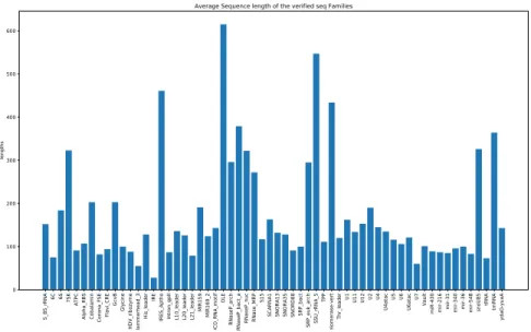
5_8 S_r RNA 6C 6S 7SK _ATPC Alp ha _R BS Cob ala min Corona _F SE Fla vi_C RE Gcv B Gly cin e HDV_rib ozy me Hamme rhe ad _3 His_l ea de r _IRE IRE S_Ap tho Intron_g pII L1 0_le ad er L2 0_le ad er L2 1_le ad er MIR 15 9 MIR1 69 _2 MOC O_R NA_motif OLE RNa se P_a rch RNa se P_b act_a RNa se P_n uc RNa se _M RP S15 SC AR NA1 SNOR A1 3 SNOR A3 5 SNOR D8 8 SR P_b act SR P_e uk_a rch SS U_rR NA_5 TPP Te lome rase -ve rt Thr_le

ader U1 U11 U12 U2 U4

U4 ata c U5 U6 U6 ata c U7 _Vault miR -43 0 mir -21 6 mir -31 mir-34 0 mir-36 mir-54 8 snoU8 5 tR NA tmR NA yd aO-yu aA families 0 100 200 300 400 500 600 leng ths

Average Sequence length of the verified seq Families

Figure 2.2 – Average length of sequences for families in training data The training data is composed of the sequences of 60 ncRNA families3

and added noise sequences. In total, there are 5520 sequences from these 60 RNA families in the training data. Detailed information of these families could be found in Supplementary Materials (AppendixA). The number of the sequences for each of these families varies between 15 and 409. The average length of sequences for each family is shown in

2. RNA sequences that their structures and their functions are verified in biology labs experi-mentally.

3. For the sake of simplicity we consider that the number of classes in the genome are known and are the same as the families in the training data (60 families).

(24)

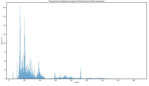
Figure2.2. Figure 2.3 depicts the frequency of the sequence lengths in training data varying between 27 and 842.

0 100 200 300 400 500 600 700 800 lengths 0 25 50 75 100 125 150 175 200 fre que ncie s

Frequencies of Sequence length of all Families of verified sequences

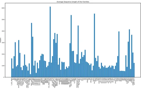
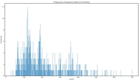
Figure 2.3 – Frequency of the sequence lengths of all families in the training data. The test data is obtained from the 10 pseudogenomes with embedded true RNA sequences. The details for the creation of these pseudogenomes could be found in Infernal’s benchmark documentation [28]. Our aim is to detect these embedded RNAs and predict correctly their labels. Information about the length of these embedded RNAs could be found in Figure 2.4 and Figure 2.5.

We represent each sequence (example) of RNA as a tuple (xi,j, yi) such that xi,jis a

vector representation of the sequence i with j features, and yiis the label providing the

RNA family to which the sequence belongs to. Regarding the sequence representation (feature vectors) we use k − mer frequency. We start with k = 3 to reduce the dimensionality of our training data since there would be 64 features (64 3_mers i.e. AAA, AAC, etc and the label) for each sequence. Later, we will try k = 4, 5, 6, 7 as well.

(25)

2.2. The model foundation 5_8 S_r RNA 6C 6S 7SK_ATPC Alp ha _R BS Ar throp od _7 SK Cob ala min Corona _F SE Corona _p k3 Fla vi_C RE Gcv B Gly cin e HDV_rib ozy me Hamme rhe ad _3 His_l ea de r_IRE IRE S_Ap tho Intron _g pI Intron_g pII L 10 _le ad er L1 9_le ad er L2 0_le ad er L2 1_le ad er Le u_le ad er Ly sin e M IR 15 9 M IR1 67 _1 MIR 16 9_2 MIR3 96 MIR4 73 MIR4 74 MOC O_R NA_motif OLE PyrR R2 _re tro_e l RNa se P_a rch RNa se P_b act_a RNa se P_n uc RNa se _M RP S15 SC AR NA1 SECIS SNOR A1 3 SNOR A3 5 SNOR D1 5 SNOR D2 5 SNOR D8 8 SNOR D9 6 SR P_b act SR P_e uk_a rch SS U_rR NA_5 SgrST-box_TLS-PK 3_TPP Te lome rase -cil Te lomera se -ve rt Thr_le

ader U1 U11 U12 U2 U3 U4

U4 ata c U 5 U6 U6 ata c U7_Vault bicoid _3 glmS isrNisrO miR -43 0 mir -10 mir-17 2 mir-21 0 mir-21 6 mir-23 9 mir-28 3 mir-31 mir-34 0 mir-36 mir-54 8 mir-81 mir-87 msr pre Q1 -II pu rD_rli28_rne5_sR13_{sR28 sR4 sR5 sR8 snR}5 sn oR 72 Y sn oU8 5 sp eF tRNA tmRNA yd aO-yu aA yy bP-ykoY families 0 100 200 300 400 500 600 leng ths

Average Sequence length of the Families

Figure 2.4 – Average length of embedded RNA sequences in the genome.

Noise generation

The noise corresponds to the regions of the genome that are not transcribed or for which the function is not known yet. These parts are usually called "dark matter" of the genome [12]. Noise sequence is simply a random sequence of nucleotides with the same length as the RNAs in the training data. So these are new observations added to the training data that correspond to nonRNA sequences in genome. So the noise portion of the training data should help to better distinguish ncRNA with nonRNA parts.

We explain the noise generation process ﬁrst regarding the multiple window length. To add the noise sequences, we take into account two things: the length of these noise sequences and their quantity4

. Since we have diﬀerent RNA families with various sequence lengths, the noise should also have diﬀerent lengths. In other words, the length of a noise sequence should be proportional to each sequence in a RNA family to look alike biologically.

For instance, the length of the sequences for Hammerhead_3 family are between

4. Number of noise sequences in the training data

(26)

2.2. The model foundation 0 100 200 300 400 500 600 700 Lengths 0 2 4 6 8 10 12 Fre que ncie s

Frequencies of Sequence length of all Families

Figure 2.5 – Frequency of the embedded RNA sequences’ lengths in the genome. (40, 82). In this situation, the noises corresponding to this family is of the lengths 40, 55, and 82. It means we add noises with the minimum, average, and maximum sequence length from each family. On the other hand, in some cases where the minimum and maximum of the lengths are so close, i.e. they have a lower standard deviation, the noises corresponding to these families are set to have a single length which is their average. Information about the number of noise sequences for each family and their lengths could be found in Table A.1 in Appendix A. The quantity of noise sequences per family is 1.5 times the sequence number of that family in the training data, i.e. if there are 100 sequences of one family, 150 noise sequences for that family is added to the training data.

We use the ﬁrst portion (pseudogenomes with length ≈ 106

nt) of our genome from

the infernal benchmark. As we said there are 10 of these pseudogenomes (rmarks) with true RNAs embedded in random positions. In order to generate the noise, we take the ﬁrst pseudogenome (rmark1) and remove those segments which are true RNAs from the 60 RNA families. Then randomly take segments with decided lengths for each family. Finally, their k − mer representation is added to the training data alongside the RNA sequences.

(27)

Regarding the single window length approach, the noise generating process is almost the same as multiple window length approach. We use rmark1 of our genome from the infernal benchmark. This time, instead of choosing noise sequences with diﬀerent length, we use sequences of single length wl (= 50nt).

2.2.2 Model selection

In order to choose the best classifier, 10-fold cross-validation is used on 75% of the training data using different classifiers from the python’s scikit-learn library [32] including K-Nearest Neighbors (KNN), Support Vector Machines (SVM), Random Forest, and Logistic Regression. The remaining 25% of the examples are used as unseen data.

Cross-validation is a re-sampling procedure used to evaluate machine learning models on a limited data sample. Cross-validation is used in applied machine learning to estimate the skill of a machine learning model on unseen data (25% of the examples in our case). That is, to use a limited sample in order to estimate how the model is expected to perform in general when used to make predictions on data (test set) not used during the training of the model.

Neighbors-based classiﬁcation is a type of instance-based learning or non-generalizing learning: it does not attempt to construct a general internal model, but simply stores instances of the training data. Classiﬁcation is computed from a simple majority vote of the nearest neighbors of each point: a query point is assigned the data class which has the most representatives within the nearest neighbors of the point [32].

Although SVM and LR are devoted to binary classification, these models imple-ment the “one-against-one” approach [29] for multi-class classification. If n_class is the number of classes, then n_class ∗ (n_class − 1)/2 classifiers are constructed and each one trains data from two classes [32]. We use support vector machines with linear, polynomial, and rbf kernels.

2.2.3 Scanning the Genome

As we know, another problem is choosing the length of the scanning window in order to extract segments to annotate (family label prediction). Since almost all ML

(28)

models work on the base of similarity, the test data (extracted segments from genome) should be similar to the training data. So the extracted segments should be in the same length of the sequences in the training data.

Regarding the MWL approach, in order to simplify the segment extraction process (shown in Figure 2.1) in the genome for each of the RNA families with different lengths, we have defined intervals of length 10 starting at 20 (i.e. 20-30, 30-40, ...) and classified these families according to their lengths in these intervals. Then the average length of families in each interval is used as a chosen scanning window length. For instance, for (90-100) length interval, we find all the RNA families that their sequence length lie in this interval. Then the average of their length is chosen for scanning window (wl) of this interval. These information could be found in Table

A.2 in Appendix A.

For each wl in Table A.2, the segments are extracted from the genome with the shift size of wl/2. Then for all generated segments, their labels are predicted. The number of the segments generated each time varies due to the diﬀerent window length (wl) and shift size (sz). In general, it is calculated using this formula:

N OS = len(genome) − wl sz

For instance, for a window length of 40, since the length of ramrk2 is 1014774, the expected number of segments generated for this window length (sz = 20) is 50738 in the scanning process. For another wl = 434, the expected number of segments is 4676.

Regarding the single window length approach, we choose a single scanning window length, wl (= 50nt), with the shift size of sz = 10 to extract segments and predict their labels.

2.2.4 Classification report

Finally, the results of the classiﬁers after 10-fold cross-validation is reported. Based on these results, we choose the best classiﬁer and proceed to the test phase. In order to evaluate the model, we chose the second pseudogenome (rmark2), of 10 pseudogenomes from the Infernal benchmark with length 1014774.

(29)

Accuracy scores and F1-score measures are used as evaluation scores. If ˆyi is

the predicted value (family label) of the i-th example (RNA sequence) and yi is

the corresponding true value, then the fraction of correct predictions over nsamples is

deﬁned as: Accuracy(y, ˆy) = 1 nsamples nsamplesX−1 i=0 1( ˆyi, yi)

The F-measure can be interpreted as a weighted harmonic mean of precision and recall. A measure reaches its best value at 1 and its worst score at 0. In this con-text, we can define the notions of precision, recall and F-measure where the terms "positive" and "negative" refer to the classifier’s prediction, and the terms "true" and "false" refer to whether that prediction corresponds to the external judgment (some-times known as the "observation"). In our context, multi-class classification task, the notions of precision, recall, and F-measures can be applied to each label indepen-dently and results are combined across the labels using the average. So RNA families are considered positive and the noise is considered negative.

precision = tp tp + f p recall = tp tp + f n F 1 = 2 · precision × recall precision + recall

Actual class (observation)

Predicted class tp (true positive) Correct result fp (false positive) Unexpected result (expectation) fn (false negative) Missing result tn (true negative) Correct absence of result

Table 2.1 – Confusion matrix.

(30)

2.2. The model foundation T able 2.2 – O ve ra ll v ie w of the us ed me tho ds and the ir re sult s Sp ec s M ult iple Windo w L eng th Sing le Windo w L eng th M et ho d1 M et ho d2 M et ho d3 M et ho d4 M et ho d5 M et ho d6 C omput at io na ly ex p ens iv e Y es (t es t pha se ) Y es (t es t pha se ) Y es No No No k _me r re pr es en ta tio n 3_me rs 3_me rs 3_me rs 3_me rs 3t o7 _me rs 5t o7 _me rs R NA re ca ll lo w lo w -hig h lo w lo w No is e re ca ll hig h hig h -lo w hig h hig h ov er all re ca ll hig h hig h -hig h hig h hig h tr aining pha se ac cur ac y hig h lo w -hig h hig h hig h

(31)

In summary, we use veriﬁed RNA and noise sequences with their labels as training data and generate vector features from these sequences using k − mer frequency representation. A machine learning model is learned on this data. Then using a scanning window based on one of the two approaches (MWL or SWL) genomes are scanned and the segments annotated. We discuss the developed methods for each of these approaches in detail in the next chapter but Table2.2 gives an overall preview of the methods.

(32)

Chapter 3 Experimental Methods and Results

In this chapter, the various methods proposed to meet the challenges that are presented. The results of each method are discussed and at the end of each method description, there is a conclusion part in which the limits of the method are reported and solutions are provided.

3.1 APPROACH1: Multiple Window Lengths

In this approach, we present diﬀerent methods for the MWL approach and discuss them in depth.

3.1.1 Method1: Multiple Window Length

In this method, we produce the 3 − mer representation of the RNA sequences that we call the sequence space. The sequence space (seq5520×64) is a matrix with 5520

objects (RNA sequences of diﬀerent families) with 64 features plus the last column which is the label showing to which family this sequence belongs. Using the noise generation method described in the previous chapter, the noise space (noise8312×64)

is also created. The training data, training_data13832×64, is then composed of both

(33)

3.1. APPROACH1: Multiple Window Lengths

Results of the classiﬁers after 10-fold cross-validation could be found in Table

3.1 and the result of the evaluation on the unseen data are shown in Table 3.2. In table 3.2 the result of Majority Voting is also included which combines the top three classiﬁers and gets the results based on the majority of the class labels predicted by each individual classiﬁer.

Classifiers Accuracy F1 KNN (k=8) 88.38 0.88 SVM - linear 90.75 0.90 SVM - poly 91.66 0.91 Random Forest(30) 85.43 0.82 Logistic regression 90.16 0.89 Table 3.1 – 10-fold cross validation - Method1.

Classifiers Accuracy F1 KNN (k=8) 88.72 0.88 SVM - linear 90.89 0.90 SVM - poly 91.55 0.91 Logistic regression 89.82 0.89 Majority Voting 93.26 0.93 KNN, SVM(linear,ploy)

Table 3.2 – Evaluation of the classiﬁers on test/unseen data - Method1. Regarding the scanning, for each wl in TableA.2, the segments are extracted from the genome with the shift size of wl/2. Then for all generated segments, their labels are predicted.

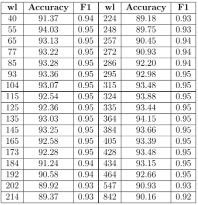
For each value of wl, using the selected classiﬁer (Majority Voting: KNN, linear and polynomial SVM), the labels are predicted for each of those segments and the recall is calculated for the embedded RNA sequences in rmark2 whose length is in the range of chosen wl. It means, for instance for Hammerhead_3 whose sequence length is in (40,82) range, the recall is calculated for the segments that are generated based on window lengths 40, 55, and 85 separately which are intervals that cover Hammerhead_3. The classiﬁcation result for this method taking into account all

(34)

3.1. APPROACH1: Multiple Window Lengths wl Accuracy F1 wl Accuracy F1 40 91.37 0.94 224 89.18 0.93 55 94.03 0.95 248 89.75 0.93 65 93.13 0.95 257 90.45 0.94 77 93.22 0.95 272 90.93 0.94 85 93.28 0.95 286 92.20 0.94 93 93.36 0.95 295 92.98 0.95 104 93.07 0.95 315 93.48 0.95 115 92.54 0.95 324 93.88 0.95 125 92.36 0.95 335 93.44 0.95 135 93.03 0.95 364 94.15 0.95 145 93.25 0.95 384 93.66 0.95 165 92.58 0.95 405 93.39 0.95 173 92.28 0.95 428 93.48 0.95 184 91.24 0.94 434 93.15 0.95 192 90.58 0.94 464 92.66 0.95 202 89.92 0.93 547 90.93 0.93 214 89.37 0.93 842 90.16 0.92

Table 3.3 – Classiﬁer result - Method1. possible window lengths1

for each segment can be found in Table 3.3. The results of Table 3.3 show really high accuracy scores.

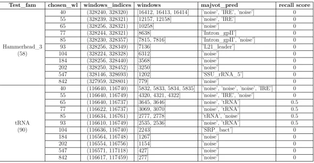
Since we are interested in detecting ncRNAs, we explore some of these predictions for families in isolation. We look at the prediction results of two specific families ’Hammerhead_3’ and ’tRNA’ in different length intervals. Also regarding the recall score, to verify the effect of window length, we take a look at the same position with different window lengths in the scanning process. It does not mean we are applying family-specific method since our training data consists of all RNA sequences.

As scanning window length increases, the number of segments should decrease. Table 3.4 includes prediction results and recall scores of two diﬀerent families ’Ham-merhead_3’ and ’tRNA’ in diﬀerent length intervals. ’Ham’Ham-merhead_3’ is embedded in (328256,328314) position with length 58 on reverse complement2

and ’tRNA’ is

1. Not all the length intervals are included. We have used the window length of the RNA families that are present at rmark2.

2. The reverse complement of a DNA sequence is formed by reversing the letters then inter-changing A and T and interinter-changing C and G. For instance the reverse complement of ACCTGAG

(35)

3.1. APPROACH1: Multiple Window Lengths embedded in (116645,116735) position with length 90.

Table 3.4 clarifies the possible problems. One problem is that the noise is not the only parameter to consider. There are some other parameters that have high influence as well. The other problem is the effect of the chosen wl on the predicted labels. This causes the wrong prediction for RNA families with shorter sequences while choosing larger window lengths. These predictions are either noise or RNA families with the same length of the chosen wl. Finally, the embedded reverse complement of some RNA sequences in pseudogenomes could be another factor to consider.

Test_fam chosen_wl windows_indices windows majvot_pred recall score

Hammerhead_3

40 (328240, 328320) [16412, 16413, 16414] [’noise’, ’IRE’, ’noise’] 0

55 (328239, 328321) [12157, 12158] [’noise’, ’IRE’] 0 65 (328256, 328321) [10258] [’noise’] 0 77 (328244, 328321) [8638] [’Intron_gpII’] 0 85 (328230, 328357) [7815, 7816] [’Intron_gpII’, ’noise’] 0 93 (328256, 328349) [7136] [’L21_leader’] 0 (58) 104 (328224, 328328) [6312] [’noise’] 0 184 (328256, 328440) [3568] [’noise’] 0 202 (328250, 328452) [3250] [’noise’] 0 547 (328146, 328693) [1202] [’SSU_rRNA_5’] 0 842 (327959, 328801) [779] [’noise’] 0 tRNA

40 (116640, 116740) [5832, 5833, 5834, 5835] [’noise’, ’noise’, ’noise’, ’IRE’] 0

55 (116640, 116749) [4320, 4321, 4322] [’noise’, ’IRE’, ’noise’] 0

65 (116640, 116737) [3645, 3646] [’noise’, ’tRNA’] 0.5 77 (116622, 116737) [3069, 3070] [’noise’, ’tRNA’] 0.5 85 (116634, 116761) [2777, 2778] [’tRNA’, ’noise’] 0.5 93 (116610, 116749) [2535, 2536] [’noise’, ’tRNA’] 0.5 (90) 104 (116636, 116740) [2243] [’SRP_bact’] 0 184 (116564, 116748) [1267] [’noise’] 0 202 (116554, 116756) [1154] [’noise’] 0 547 (116571, 117118) [427] [’noise’] 0 842 (116617, 117459) [277] [’noise’] 0

Table 3.4 – Behaviour of Method1 in diﬀerent window lengths for tRNA and Ham-merhead_3.

From these observations, we see that the inﬂuence of the sequence length combined with noise factor make the prediction incorrect. Adding noises with diﬀerent lengths makes the problem harder since for 3 − mer representation shorter sequences have fewer counts of 3 − mers while longer sequences have larger frequencies.

is CTCAGGT.

(36)

Conclusion and perspective

Based on these results, we see that the model (chosen classifier) is not able to distinguish between RNAs and noises for most of the families. Knowing the signifi-cance of length, we try to normalize it in order to reduce its influence. One solution to normalize is by dividing the frequency of each 3_mer xi,j by the length of the ith

sequence. In order to detect other inﬂuencing parameters, an in-depth analysis is conducted to get more insight into the data. For the rest of the section 3.1, we take a closer look at data and possible parameters like reverse complement and length. We try another method that includes normalizing the length and also we take into account the fact that some of the RNA sequences have been embedded in their reverse complement form. Our hypothesis is that since each sequence and its reverse com-plement has totally diﬀerent k − mer representation, we hope including both in the training data may increase the evaluation metrics like recall. Details of this method will be discussed in the following section.

3.1.2 Method2: Multiple Window Length normalized with

the sequence length and taking into account the reverse

complement

In this method, we normalize the training data by dividing the value of each 3 −

mer by the sequence length l. Moreover, to take into account the reverse complement,

the 3−mer representation of the reverse complement for each sequence in the training data is added. This means the size of the training data will be doubled which may increase the complexity and the computation time.

To deal with this matter, four RNA families are selected, tRN A, U 5, M IR159, and tmRN A, to be examined thoroughly so the training data includes a single-family and the noise. This is exactly the family-speciﬁc strategy. The criteria for choosing these families are based on their sequence quantity in training and test data and their length range. For each of these four families, the training data includes the 3 − mer representation of the sequence i and its reverse complement as well as noise data generated from rmark1 using the same procedure as for Method1 3.1.1. The model is trained on this training data and ﬁnally, at the test phase, the predicted results for

(37)

corresponding and also other window length intervals are provided.

Classifiers Accuracy F1 KNN (k=5) 80.48 0.80 SVM - linear 48.24. 0.34 SVM - poly 43.03. 0.25 SVM - rbf 43.03 0.25 Random Forest(30) 94.05 0.93 Logistic regression 47.77 0.33 Table 3.5 – 10-fold cross validation - Method2.

The classifiers are then applied to the generated training data (Tables3.5and3.6). Except for Random Forest, all other classifiers perform poorly so the majority voting is not used in this case. Then labels are predicted using the best classifier for extracted segments. For each window length (wl), chosen for scanning, the generated segments are normalized by wl. Reverse complement of the segments are not generated in the test data.

Classifiers Accuracy F1

KNN (k=5) 81.89 0.82

Random Forest (30) 95.18 0.95 Table 3.6 – Evaluation of the classiﬁers - Method2.

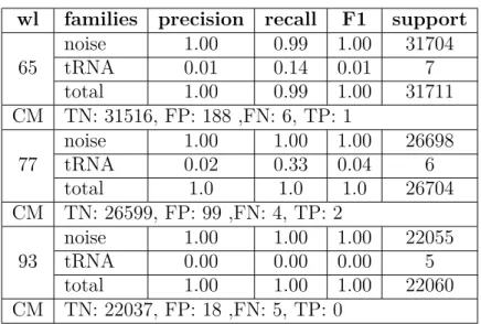
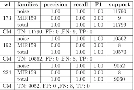
We examine one family at a time versus noise. The classiﬁcation results for these experiments are provided in Tables3.7-3.10. The results include recall, precision, F1 score, and the "support" which indicates the number of segments in each class after scanning with the chosen window length. The confusion matrix is also provided. By examining these results, we see that for almost all of these families the true positive value is zero, which means the classiﬁer reports the RNA as noise.

It appears clearly that Approach1 is not able to yield the expected output. Besides all the challenges related to noise and window length, wl, the fact that the scanning process should be done for each of these wl intervals separately is a hassle. All these obstacles are strong shreds of evidence for not investing in this approach (MWL).

Tables 3.7-3.10 show no improvements using this method compared to Method1. So normalizing with the sequence length and including reverse complement in the

(38)

wl families precision recall F1 support

65 noise 1.00 0.99 1.00 31704 tRNA 0.01 0.14 0.01 7 total 1.00 0.99 1.00 31711 CM TN: 31516, FP: 188 ,FN: 6, TP: 1 77 noise 1.00 1.00 1.00 26698 tRNA 0.02 0.33 0.04 6 total 1.0 1.0 1.0 26704 CM TN: 26599, FP: 99 ,FN: 4, TP: 2 93 noise 1.00 1.00 1.00 22055 tRNA 0.00 0.00 0.00 5 total 1.00 1.00 1.00 22060 CM TN: 22037, FP: 18 ,FN: 5, TP: 0

Table 3.7 – Classiﬁer result including tRNA and noise.

104 noise 1.00 1.00 1.00 19503 U5 0.00 0.00 0.00 11 total 1.00 1.00 1.00 19514 CM TN: 19503, FP: 0 ,FN: 11, TP: 0 115 noise 1.00 1.00 1.00 17792 U5 0.00 0.00 0.00 11 total 1.00 1.00 1.00 17803 CM TN: 17789, FP: 3 ,FN: 11, TP: 0 135 noise 1.00 1.00 1.00 15135 U5 0.00 0.00 0.00 10 total 1.00 1.00 1.00 15145 CM TN: 15135, FP: 0 ,FN: 10, TP: 0

Table 3.8 – Classiﬁer result including U5 and noise.

training data did not lead to any diﬀerence. It means we should seek the answer elsewhere.

3.1.3 Conclusion and perspective

Length of scanning window, shift size, noise generation, noise quantity, and the reverse complement of the sequence are the challenges we started with. These

(39)

vari-3.1. APPROACH1: Multiple Window Lengths

173 noise 1.00 1.00 1.00 11790 MIR159 0.00 0.00 0.00 9 total 1.00 1.00 1.00 11799 CM TN: 11790, FP: 0 ,FN: 9, TP: 0 192 noise 1.00 1.00 1.00 10562 MIR159 0.00 0.00 0.00 8 total 1.00 1.00 1.00 10570 CM TN: 10562, FP: 0 ,FN: 8, TP: 0 224 noise 1.00 1.00 1.00 9052 MIR159 0.00 0.00 0.00 8 total 1.00 1.00 1.00 9060 CM TN: 9052, FP: 0 ,FN: 8, TP: 0

Table 3.9 – Classiﬁer result including MIR159 and noise.

315 noise 1.00 1.00 1.00 6447 tmRNA 0.00 0.00 0.00 16 total 1.00 1.00 1.00 6463 CM TN: 6447, FP: 0 ,FN: 16, TP: 0 364 noise 1.00 1.00 1.00 5561 tmRNA 0.00 0.00 0.00 14 total 0.99 1.00 1.00 5575 CM TN: 5560, FP: 1 ,FN: 14, TP: 0 405 noise 1.00 1.00 1.00 5009 tmRNA 0.00 0.00 0.00 14 total 0.99 1.00 1.00 5023 CM TN: 5009, FP: 0 ,FN: 14, TP: 0

Table 3.10 – Classiﬁer result including tmRNA and noise.

ous parameters and challenges affect the model differently in isolation and together. The model improvements did not handle all these obstacles and so far, from these challenges, length plays an important role. Using different window lengths requires multiple scans for each wl which is a big challenge that lingers whichever if the perfect model was found.

Now we move to the second approach that uses a single window length to eliminate

(40)

the eﬀect of length. For this approach, the other challenges still exist as well. Besides, the sequences may look more alike by just using the same length for all.

(41)

3.2. Approach2: Single Window Length

3.2 Approach2: Single Window Length

In this section, we deﬁne possible solutions for length, noise quantity, and the reverse complement by using single window length to control existing challenges. First of all, we deﬁne what we mean by "single" window length and how it is possible to represent these sequences with various lengths using just one length.

The main idea behind single window is similar to the scanning process (Figure

2.1). For each sequence S = s1s2...sl with length l, starting at position i = 1, we take

segments of length wl (window length), i.e. seg = sisi+1...si+wl. Then by repeating

this process by shifting the start position i along the sequence, i = i + sz (shift size), the next segment is generated. For instance for wl = 50 and sz = 10, following segments are generated: seg1 = s1s2...s50, seg2 = s11s12...s60 and so on. Hence, each

sequence S would be replaced by segment chunks of the original sequence. For a sequence S with length l the number of segments (NOS) generated with length wl and shift size sz are:

N OS = l − wl sz

This means the number of the sequences in the training data increases since each sequence is replaced with N OS sub-sequences generated by this notion. We refer to this process as sequence "segmentation". Segmentation process looks exactly like the scanning process depicted in Figure2.1. In other words, each sequence in the training data is replaced by all the segments (NOS) extracted using this segmentation process oﬀ that sequence.

Regarding the noise generation and its quantity, it is generated randomly and the quantity of the noise will depend on the situation and the number of the segments generated from each sequence. Furthermore, the reverse complement is not generated for every single sequence in the training data. However, in the test phase for each segment, the labels are predicted for both the segment and its reverse complement. So this also eliminates the complexity and the confusion of having both sequence and its reverse complement in the training data.

(42)

3.2.1 Method3: Single window length

We regenerate the same training data in 3.1.1 satisfying conditions for current method. Each sequence of RNA in the training data is segmentized with wl = 50 and

sz = 10 so the families and sequences smaller than 50 are eliminated. Based onA.1,

IRE entirely and Hammerhead_3 is partially eliminated. N OS could be calculated

using the formula above. For instance for a sequence of length l = 130, N OS is 7. This means a sequence with length 130, will be replaced by 7 sequences with length 50 and the training data consists of their k − mer representation.

N OS = 123 − 50

10 = 7

The training_data106042×65 is composed of 97730 segments generated by the

seg-mentation process of RNA sequences and 8312 noises (random segments of rmark1 with length 50). Notice that the same quantity of noise as Method1 in section 3.1 is included (1.5 times of sequences per family).

Following the same habit of choosing the classifier using 10-fold cross-validation, a classifier was not able to be trained on the generated training data (i.e. the program did not end after running for a long time). The reason for this is due to the increase in the number of sequences in the training data that they look alike due to the overlap (as a result of segmentation) which makes it difficult for the classifiers. Another possible reason is that due to high similarity between the sequences, 64 features are not enough to distinguish these sequences, i.e. short sequences do not tend to have significant differences in terms of 3 − mer frequencies.

In order to reduce the number of sub-sequences in the training data, we could use a certain number of sequences from each family as initial seed (init_seq) and generate the segments just for those initial sequences or deﬁne a threshold for the number of segments produced after segmentation process for each family.

(43)

3.2.2 Method4: Single window length with upper limit for

generated segments

There are different ways to reduce the computational complexity of the program. One is choosing a specific number of examples (RNA sequences) from each family for the segmentation process which causes different number of N OS values for each RNA family. This means families containing shorter sequences tend to generate fewer segments of single length 50 and on the other hand families with longer sequences would result in a larger number of the segments. As a result, since the length of the sequences of RNA families are different, each family will produce a various number of segments using the same initial number of sequences. This may result in imbalanced data due to the fact that the length of these sequences vary.

In order to approach this challenge, we suggest having an upper limit (init_seg) for the total number of the segments that are generated for each family after segmen-tation. Using this method, the number of the elements for each class (RNA family) would be more alike. This means although the number of segments from diﬀerent families does not vary, some families utilize a small number of their RNA sequences to generate the same number of single-length segments.

init_seg is deﬁned as a maximum number of segments that each family could have

in the training data regardless of their original sequence quantity. With init_seg = 250, the variation of generated segments is high so we choose init_seg = 150. The comparison between the number of sequences of each family and generated segments using an upper limit of 250 and 150 is shown in TableA.3. The column "original data" indicates the number of sequences in each RNA family at the beginning (original ﬁle). Then we show the number of sequences that are used from each family to generate

init_seg segments.

Based on these results we proceed with init_seg = 150 which reduces the number of segments from diﬀerent families to 7923. We reduced the number of noises to 200 (10% of the seq space) since there is a maximum of 150 elements from each RNA family. Like all other methods, cross-validation is used to choose the best classiﬁer. These results are shown in Tables 3.11 and 3.12.

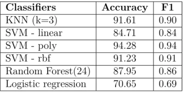
SVM poly is chosen for predicting the labels of segments after scanning. Classiﬁ-32

(44)

3.2. Approach2: Single Window Length Classifiers Accuracy F1 KNN (k=3) 91.61 0.90 SVM - linear 84.71 0.84 SVM - poly 94.28 0.94 SVM - rbf 91.23 0.91 Random Forest(24) 87.95 0.86 Logistic regression 70.65 0.69 Table 3.11 – 10-fold cross validation - Method4.

Classifiers Accuracy F1 KNN (k=3) 92.81 0.91 SVM - poly 94.53 0.94 SVM - rbf 92.22 0.92 Majority Voting 94.24 0.93 (knn,svm poly,svm rbf)

Table 3.12 – Evaluation of the classiﬁers - Method4.

cation results using this classiﬁer for both normal and reverse complement of segments is shown in Tables 3.13 and 3.14. These results just include the four families that are chosen in the previous approach (3.1) since including the results for all families would take lots of space. These classes represent RNAs of diﬀerent lengths so they are reliable for future interpretation.

Comparing the recall scores in Tables 3.13 with the results from 3.1 we see that although overall results decreased (due to low noise recall), the recall scores for some of the families are improved and some of the segments that were missed completely are predicted correctly but recall value for noise is decreased. This shows that the model has diﬃculties distinguishing between noise and true RNA. Furthermore, low precision scores indicate that more true families are misclassiﬁed either as other classes or noise. This may indicate that 3 − mers representation is not the best choice. A closer look at the predicted labels using Method4 proves these ideas.

Results in3.15for tRNA, mir-31, and L20_leader show how Method4 is improved. Speciﬁcally for tRNA compared to 3.4 in Method1. Another interesting thing is the prediction of Alpha_RBS for L20_leader segments while these two families are not even in the same length range. Table A.1 shows that Alpha_RBS sequences length

(45)

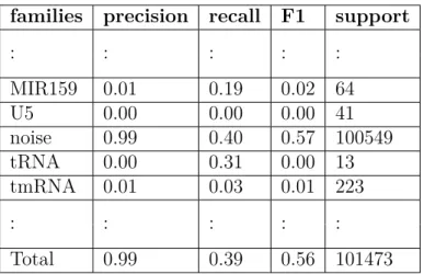
Table 3.13 – Classiﬁer result - Method4.

families precision recall F1 support

: : : : : MIR159 0.01 0.19 0.02 64 U5 0.00 0.00 0.00 41 noise 0.99 0.40 0.57 100549 tRNA 0.00 0.31 0.00 13 tmRNA 0.01 0.03 0.01 223 : : : : : Total 0.99 0.39 0.56 101473

Table 3.14 – Classiﬁer result - Method4 with rc.

families precision recall F1 support

: : : : : MIR159 0.01 0.12 0.01 64 U5 0.00 0.00 0.00 41 noise 0.99 0.40 0.57 100549 tRNA 0.00 0.00 0.00 13 tmRNA 0.01 0.03 0.01 223 : : : : : Total 0.98 0.39 0.56 101473 34

(46)

are in (88-119) range where L20_leader includes sequences with length (119-134). The same condition happened in U5 and OLE cases but SNORA35 and SNORA13 have almost the same sequence length. Again this demonstrates that for segments of length 50, 3 − mers are not able to make diﬀerence.

Family Length Method4 recall

tRNA 90 [’tmRNA’, ’tRNA’, ’tRNA’, ’tRNA’, ’tRNA’] 0.8

mir-31 78 [’U6’, ’mir-31’, ’mir-31’] 0.66

U5 110 [’mir-548’, ’noise’, ’OLE’, ’SNORA35’, 0

’SNORA13’, ’noise’, ’noise’]

L20_leader 126 [’L20_leader’, ’L20_leader’, ’noise’, ’Alpha_RBS’, 0.22 ’Alpha_RBS’,’Alpha_RBS’, ’noise’, ’Alpha_RBS’,

’GcvB’]

Table 3.15 – Predicted label for some of the sequences using Method4.

In summary, families, and noise are not perfectly distinguishable but recall values for families are increased. Decreased recall score for noise means the noise parts of the genome are labeled as RNA. One possibility is overlapping due to small shift size(sz = 10). The stronger possibility is the representation of these sequences (3−mers). Since a fixed length of 50 is chosen, which is respectively short, the chances that these segments would have totally different 3 − mer frequencies are low and overlapping caused by small shift size intensifies this problem. The main reason for choosing k = 3 is the small number of produced features. Using 3−mers we have 64 features however using 4, 5, or 6_mers increases the number of features and hence the dimensionality. For the final attempt, the frequent patterns of the length {3,4,5,6,7} are used. We discuss the details for the methods based on this idea in the following sections.

3.2.3 Method5: Single window length with reduced (1000)

frequent patterns

We found the most frequent k − mers of k = {3, 4, 5, 6, 7} overall in all sequences as well as per family. The frequency of the most frequent patterns in all sequences

(47)

(seq space) is shown in table 3.16. We can see that all of them are 3 − mers. Table

3.17 shows the top frequent pattern for each RNA family.

Occurrence Patterns 91703 GGG 86245 AGG 83776 AAA 83023 CGG 81041 GGC 80761 GGA 80731 GGU 80086 AAG 79653 GAA 77399 GAG 75982 GCC 75088 CCG 72944 UUU 72783 GCA

Table 3.16 – Top frequent patterns in all sequences.

Table 3.17: Top frequent patterns per family. Begin of Table

Family Patterns Occurrence

SRP_euk_arch GGG 2603 Flavi_CRE CAG 1008 noise AUA 9194 His_leader AAA 533 IRES_Aptho ACU 5948 RNaseP_bact_a CGG 17032 U6 AGA 3229 HDV_ribozyme GGC 303 ydaO-yuaA GGG 2718 mir-31 GCU 311 36

(48)

Continuation of Table 3.17

snoU85 UGU 732 U11 UUU 1132 GcvB UUU 874 SRP_bact AGC 5892 MOCO_RNA_motif GCC 1835 mir-216 CUG 231 RNaseP_nuc GGG 3847 U1 GGG 2124 5_8S_rRNA GAA 1662 Alpha_RBS UUU 419 SSU_rRNA_5 AAU 14618 RNase_MRP GCG 1322 Glycine AGG 321 7SK UCC 2495 OLE AAA 1653 TPP UGA 1580 L10_leader UUU 725 U2 UUU 6108 Telomerase-vert CGC 1916 Thr_leader AAA 610 L20_leader UUU 390 SNORD88 CCC 680 U6atac ACA 993 MIR159 UGA 1057 mir-36 GGU 376 U4atac UUU 769 Intron_gpII GGG 994 L21_leader UUU 225 ATPC AAA 1549

(49)

Continuation of Table 3.17

Corona_FSE UGU 203 SNORA13 UUU 1056 6S CCU 787 tRNA GGU 5474 tmRNA AAA 5505 Hammerhead_3 UGA 467 U4 UUU 4295 6C CCC 644 Cobalamin CCG 12083 SNORA35 GCA 447 U12 UUU 874 mir-340 UGU 530 Vault UUC 873 U5 UUU 3797 RNaseP_arch GAA 1220 U7 UUU 547 mir-548 AAA 974 S15 AAA 1503 MIR169_2 UUU 992 SCARNA1 UGU 741 miR-430 UUU 537 End of Table3.17

Since the frequency of patterns is aﬀected by the number of sequences and their length, we choose the top 100 frequent patterns in each family and choose the union of these frequent patterns. Overall, from these top 100 patterns of each family, 1064 frequent patterns are selected. Table 3.18 shows the number of selected frequent patterns from each k − mer group.

Almost all the 3 − mers and 4_mers are frequent in all families so they may not be informative. We reduce the dimensionality by eliminating the features that

aliFreeScan: une approche sans alignement pour annoter l’ARN non codant dans des données génomiques à l'aide d'apprentissage machine