HAL Id: tel-01456470
https://tel.archives-ouvertes.fr/tel-01456470
Submitted on 5 Feb 2017HAL is a multi-disciplinary open access archive for the deposit and dissemination of sci-entific research documents, whether they are pub-lished or not. The documents may come from teaching and research institutions in France or abroad, or from public or private research centers.
L’archive ouverte pluridisciplinaire HAL, est destinée au dépôt et à la diffusion de documents scientifiques de niveau recherche, publiés ou non, émanant des établissements d’enseignement et de recherche français ou étrangers, des laboratoires publics ou privés.
Detection and classification of type Ia supernovae for
cosmology in the complete data set of SNLS
Anais Möller
To cite this version:
Anais Möller. Detection and classification of type Ia supernovae for cosmology in the complete data set of SNLS. Cosmology and Extra-Galactic Astrophysics [astro-ph.CO]. Université Paris Diderot (Paris 7), 2015. English. �tel-01456470�
Th`ese pr´epar´ee `a l’UNIVERSIT´E PARIS DIDEROT ´
Ecole doctorale STEP’UP - ED N 560
CEA Saclay Irfu/SPP Cosmologie
D´
etection et classification des supernovae de type Ia pour
la cosmologie dans l’ensemble des donn´
ees de SNLS
par
Anais M¨oller
present´ee et soutenue publiquement le 28 septembre 2015
Th`ese de doctorat de Physique de l’Univers dirig´ee par Vanina Ruhlmann-Kleider
devant un jury compos´e de:
LIDMAN Chris Rapporteur Astronomer (Australian National Observatory)
MAGNEVILLE Christophe Rapporteur Physicien senior (CEA Saclay Irfu/SPP)
GRENIER Isabelle President du jury Professeur (Paris Diderot)
LE GUILLOU Laurent Membre Maˆıtre de conf´erences (UPMC/LPNHE)
PAIN Reynald Membre Directeur de recherche (LPNHE-CNRS)
STARCK Jean-Luc Membre Directeur de recherche (CEA Saclay Irfu/SAp )
RUHLMANN-KLEIDER Vanina Directrice de th`ese Directeur de recherche (CEA Saclay Irfu/SPP)
Universit´
e Sorbonne Paris Cit´
e
UNIVERSIT´E PARIS DIDEROT ´
Ecole doctorale STEP’UP - ED N 560
CEA Saclay Irfu/SPP Cosmologie
Detection and classification of type Ia supernovae for
cosmology in the complete data set of SNLS
by
Anais M¨oller
presented on September 28th, 2015
PhD on physics
supervised by Vanina Ruhlmann-Kleider
Jury:
LIDMAN Chris Referee Astronomer (Australian National Observatory)
MAGNEVILLE Christophe Referee Senior physicist (CEA Saclay Irfu/SPP)
GRENIER Isabelle President of the jury Professor (Paris Diderot)
LE GUILLOU Laurent Member Maˆıtre de conf´erences (UPMC/LPNHE)
PAIN Reynald Member Research director (LPNHE-CNRS)
STARCK Jean-Luc Member Research director (CEA Saclay Irfu/SAp )
RUHLMANN-KLEIDER Vanina PhD supervisor Research director (CEA Saclay Irfu/SPP)
dos por barandas baj´ısimas. [. . . ] Quiz´a me enga˜nen la vejez y el temor, pero sospecho que la especie humana -la ´unica- est´a por extinguirse y que la Biblioteca perdurar´a: ilumi-nada, solitaria, infinita, perfectamente inm´ovil, armada de vol´umenes preciosos, in´util, incorruptible, secreta.”
Abstract
Detection and classification of type Ia supernovae for cosmology in the complete data set of SNLS
by Anais M¨oller
In this work, I present improvements on the detection of transient events and the classi-fication of supernovae (SNe) using supernova photometric redshifts in the SNLS deferred analysis. Detection of transient events can provide numerous false detections, while the photometric classification of type Ia SNe is usually contaminated by other types of SNe. Reducing the number of false detections and the misclassified SNe while maintaining the type Ia SN sample are important issues for both present and future surveys.
In order to reduce the artifacts that provide false detections, I developed a subtracted image stack treatment to reduce the number of non SN-like events using morphological component analysis. This technique exploits the morphological diversity of objects to be detected to extract the signal of interest. At the level of our subtraction stacks, SN-like events are rather circular objects while most spurious detections exhibit di↵erent shapes. SNIa Monte-Carlo (MC) generated images were used to study detection efficiency and coordinate resolution. When tested on SNLS 3-year data this procedure decreases the number of detections by a factor of two, while losing only 10% of SN-like events, almost all faint ones. MC results show that SNIa detection efficiency is equivalent to that of the original method for bright events, while the coordinate resolution is slightly improved. The deferred pipeline uses only photometric information to classify SNe. The advantages of a photometric sample include larger number of events classified as type Ia, larger redshift coverage and no need for spectroscopic observations. I present here a new classification using photometric supernova redshifts optimized by a machine learning classification strategy. This algorithm provides redshifts for all events with a better average precision and lower catastrophic errors than the host galaxy photometric redshift catalogue used in the SNLS3 analysis. I optimized the selection strategy using machine learning techniques such as BDTs which increases efficiency and purity of the SNIa sample. This new photometric SN-redshift classification provides a type Ia SN sample with a contamination of less than 10% according to Monte-Carlo studies.
D´etection et classification des supernovae de type Ia pour la cosmologie dans l’ensemble des donn´ees de SNLS
par Anais M ¨OLLER
Dans cette th´ese, je pr´esente des am´eliorations sur la d´etection d’ev´enements transitoires et la classification des supernovae (SNe) en utilisant les redshifts photom´etriques de supernova dans l’analyse dif´err´e de SNLS. La d´etection des ´ev´enements transitoires peut fournir de nombreuses fausses d´etections, tandis que la classification photom´etrique des SNe de type Ia est g´en´eralement contamin´e par d’autres types de supernovae. R´eduire le nombre de fausses d´etections et les SNe malclass´es tout en maintenant l’´echantillon du type Ia sont des questions importantes pour les investigations pr´esentes et futures. Afin de r´eduire les artefacts qui fournissent des fausses d´etections, j’ai d´evelopp´e un traitement pour les stacks des images soustraites pour r´eduire le nombre d’´ev´enements qui ne se ressamblent a SNe en utilisant Morphological Component Analysis. Cette technique exploite la diversit´e morphologique des objets `a d´etecter pour extraire le signal d’int´erˆet. Au niveau de nos piles de soustraction, ´ev´enements comme SN sont plutˆot circulaires alors que la plupart des d´etections parasites pr´esentent des formes di↵´erentes. Images des SNe Ia g´en´er´ees par Monte-Carlo (MC) ont ´et´e utilis´es pour ´etudier l’efficacit´e de la d´etection et la r´esolution des coordonees. Lors d’un essai sur le donn´ees SNLS des 3 ans cette proc´edure diminue le nombre de d´etections par un facteur de deux, tout en ne perdant que 10 % d’´ev´enements qui se ressamblent au SNe, presque tous faibles. R´esultats des MC montrent que l’efficacit´e de d´etection SNIa est ´equivalente `a celle de la m´ethode originale pour les ´ev´enements lumineux, tandis que la r´esolution de coordonn´ees est l´eg`erement am´elior´ee.
L’analyse di↵´er´e utilise uniquement des informations photom´etriques pour classer les supernovae. Les avantages d’un ´echantillon photom´etrique comprennent plus grand nombre d’´ev´enements class´es comme de type Ia, la couverture de redshift plus grande et pas besoin d’observations spectroscopiques. Je pr´esente ici une nouvelle classification en utilisant redshifts photom´etriques de supernovae optimis´ees par une strat´egie de classi-fication avec machine learning. Cet algorithme fournit des d´ecalages vers le rouge pour tous les ´ev´enements avec une meilleure pr´ecision moyenne et inf´erieure erreurs catas-trophiques que l’analyse avec photom´etrique redshifts de la galaxie hˆote avec SNLS3. J’ai optimis´e la strat´egie de s´election `a l’aide des techniques de machine learning comme BDTs que augmente l’efficacit´e et la puret´e de l’´echantillon SNIa. Cette nouvelle clas-sification photom´etrique SN-redshift fournit un ´echantillon des SNe type Ia avec une contamination de moins de 10 % selon les ´etudes de Monte-Carlo.
Contents
Abstract ii
Resum´e iii
Contents iv
List of Figures vii
List of Tables xi
Abbreviations xii
1 Introduction 1
2 Physical Universe: cosmology and acceleration of expansion 4
2.1 Rise of General Relativity . . . 5
2.2 Symmetry: Cosmological Principle . . . 7
2.3 Space: Manifolds and metric . . . 7
2.4 Dynamic universe: Friedmann-Lemaˆıtre-Robertson-Walker Metric. . . 9
2.5 Expanding universe. . . 10
2.6 Universe’s content . . . 14
2.6.1 Matter: baryons and dark matter. . . 14
2.6.2 Radiation . . . 15
2.6.3 Dark energy as a homogeneous fluid . . . 16
2.7 Friedmann equations . . . 17
2.8 ⇤CDM . . . 18
3 Cosmological Observable: Supernovae of type Ia 21 3.1 Supernovae . . . 21 3.1.1 Empirical classification. . . 22 3.2 Supernovae of type Ia . . . 23 3.2.1 Spectroscopic properties . . . 24 3.2.2 Photometric properties . . . 25 3.2.3 Standardizing SNeIa . . . 28 3.2.4 SN Ia rates . . . 30 3.2.5 Proposed mechanisms . . . 31
3.2.5.1 Single degenerate model (SD) . . . 32
3.2.5.2 Double degenerate model (DD). . . 33 iv
3.3 Distance measurements with SNe Ia . . . 33
4 SuperNova Legacy Survey (SNLS) 36 4.1 The instrument . . . 36
4.2 SNLS survey . . . 37
4.3 The pipelines . . . 41
5 SNLS deferred photometric analysis 44 5.1 Image Processing . . . 45
5.1.1 Astrometry and resampling . . . 45
5.1.2 Subtractions . . . 46
5.2 Detection of transient events . . . 49
5.2.1 Lunation stacks. . . 50
5.2.2 Detection catalogues . . . 50
5.2.3 Detection efficiency for SNLS3 . . . 51
5.3 Selection of SN-like events . . . 53
5.3.1 Light curve reconstruction . . . 53
5.3.2 SN-like cuts . . . 55
5.4 SN classification: type Ia selection . . . 57
5.4.1 SALT2 and photometric host-galaxy redshift . . . 58
5.4.2 Light curve sampling requirements . . . 59
5.4.3 Using SALT2 parameters for SNIa selection . . . 59
5.5 5-year analysis changes. . . 63
5.6 Summary . . . 64
6 A brief introduction to signal processing and sparsity 66 6.1 Basic concepts: sparsity, atom, dictionary and scales . . . 67
6.2 Morphological diversity . . . 69
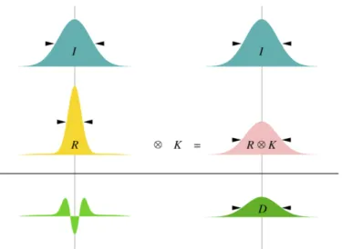
6.3 Morphological Component Analysis. . . 70
6.4 Dictionaries . . . 71
6.4.1 From Fourier to wavelet . . . 71
6.4.2 Two-dimensional wavelets . . . 73
7 Improving detection of transient events 77 7.1 Subtracted image stacks defects . . . 78
7.2 Disentangling real transient events from artifacts . . . 82
7.2.1 Choice of dictionaries . . . 82
7.2.2 First treatment: removal of main artifacts . . . 84
7.2.3 Second treatment: signal extraction with varying noise . . . 88
7.3 New Detection strategy . . . 90
7.3.1 Validating a detection . . . 93
7.3.2 Assigning coordinates . . . 94
7.3.3 Improving coordinate resolution . . . 95
7.4 Results with SNLS3 data . . . 97
7.5 MC studies . . . 98
7.5.1 Corrections: Isolation . . . 98
7.5.2 Corrections: Redshift and SNIa rate distributions. . . 99
Contents vi
7.6 SNLS and beyond... . . 105
7.7 Summary . . . 106
8 Classification of SNe Ia using photometric redshifts 108 8.1 Machine learning and boosted decision trees . . . 109
8.1.1 Principles . . . 109
8.1.2 TMVA. . . 112
8.2 Considerations for our application . . . 112
8.2.1 Samples used in the BDT set-up and analysis . . . 114
8.2.2 BDT analysis set-up . . . 116
8.2.2.1 Finding the appropiate hyperparameters . . . 116
8.2.2.2 Choosing a set of classification variables . . . 118
8.2.2.3 Choice of the BDT response threshold . . . 119
8.3 Classification of SNe Ia using photometric redshifts . . . 122
8.4 Host-galaxy photometric redshift analysis (zgal). . . 123
8.4.1 zgal + SALT2 + sequential cuts: SNLS3. . . 124
8.4.2 zgal + SALT2 + BDT analysis . . . 125
8.5 SN photometric redshift analysis (zpho) . . . 132
8.5.1 Classification using SALT2 twice (zpho+SALT2) . . . 134
8.5.1.1 zpho + SALT2 + sequential cuts analysis . . . 134
8.5.1.2 zpho + SALT2 + BDT analysis . . . 136
8.5.2 zpho + general fit + BDT analysis . . . 141
8.6 Summary . . . 148
9 Conclusions 152
A Resum´e du travail en francais 154
Bibliography 161
2.1 Galaxy distribution from 2dFGRS and SDSS . . . 8
2.2 Original diagram by Hubble in 1929 . . . 11
2.3 Comparisson H0 measurements by Planck 2015.. . . 11
2.4 Hubble diagram from the Supernova Cosmology Project . . . 16
2.5 E↵ect dark energy models on H and dL . . . 19
2.6 ⌦⇤ vs. ⌦m confidence contours of the JLA analysis . . . 20
3.1 SNe spectra and light curves . . . 23
3.2 Image of a galaxy with a SNIa . . . 23
3.3 SNIa spectrum for SN1981b . . . 24
3.4 SNIa light curve from SNLS . . . 26
3.5 Calan Tololo light curves with correction. . . 26
3.6 SNe Ia properties correlations as seen by SNLS . . . 29
3.7 Stretch and color of SNLS SNIa light curves as a function of their host galaxy stellar mass . . . 29
3.8 Observed SN Ia volumetric rate evolution with fitted parameters for the two parameter model . . . 31
4.1 CFHT dome. . . 37
4.2 The MegaPrime instrument . . . 37
4.3 MegaCam imager . . . 38
4.4 MegaCam filter transmission curves . . . 39
4.5 Full sky map with position of the deep and wide fields of CFHTLS . . . . 39
4.6 MegaCam e↵ective passbands at the center of the focal plane . . . 40
4.7 Light curves for SNLS SN Ia candidates . . . 41
4.8 JLA Hubble diagram . . . 43
5.1 Example of using subtraction for detecting SNe Ia . . . 47
5.2 Reference image for field D1 . . . 48
5.3 Image subtraction principle with a PSF adjustment. . . 49
5.4 Sketch: detection of transient events as in SNLS3 for each virtual CCD . 51 5.5 Detection efficiency for SNe Ia as a function of the generated iM peak magnitude in all survey fields. . . 53
5.6 Di↵erence in the reduced 2 between i M light curve fits by a constant and by an SN-like shape . . . 55
5.7 SN-like selection cuts applied on SNLS3 . . . 57
5.8 SALT2 parameters plot for color and stretch . . . 61
5.9 Color-magnitude diagrams . . . 62
5.10 E↵ect of the SNIa selection cuts. . . 63 vii
List of Figures viii
5.11 Distribution of host-galaxy photometric redshifts for photometrically
se-lected SNe Ia in SNLS3 . . . 65
6.1 Example of signals in time and Fourier space . . . 68
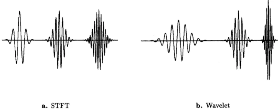
6.2 Basis functions for STFT and wavelet transform . . . 72
6.3 NGC2997 starlet decomposition . . . 73
6.4 Simulated Hubble Space Telescope image of a distant cluster of galaxies . 74 6.5 Example of curvelet . . . 74
6.6 Ridgelet example . . . 75
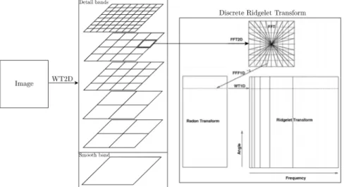
6.7 Flowchart of image decomposition in the discrete ridgelet dictionary . . . 75
6.8 Decomposition flowchart of an image in the first-generation discrete curvelet dictionary . . . 76
7.1 Reference image for field D1 . . . 79
7.2 Detection map for field D4 in SNLS3 . . . 79
7.3 Di↵erent defects on the subtracted image stacks on large scale. . . 80
7.4 Di↵erent defects on the subtracted image stacks on small scale . . . 80
7.5 Image stack for field D4, ccd 00 and lunation 10 . . . 81
7.6 SN 04D1c with its host-galaxy and after subtraction . . . 83
7.7 Typical atoms from the dictionaries used in the MCA algorithm . . . 83
7.8 MCA decomposition of a optical ghost . . . 85
7.9 MCA Decomposition of a SN Ia event . . . 85
7.10 Varying noise: pixel content in a 50x50 pixels box at di↵erent locations in a subtracted image stack . . . 86
7.11 MCA Decomposition of a SN Ia event where part of the signal leaks into the residuals. . . 87
7.12 Image stack before and after first treatment . . . 88
7.13 Varying noise after first treatment . . . 89
7.14 SNIa in the original subtracted image stack and after both treatments . . 91
7.15 Image stack for field D4 original, after first treatment and after two-step . 91 7.16 New detection strategy schema . . . 92
7.17 A SNIa event in the original subtracted image stacks and after cleaning . 93 7.18 Number of pixels required to validate a detection: # lost events vs. # detections . . . 94
7.19 Detection maps for field D4 in SNLS3 . . . 96
7.20 Detection efficiency versus isolation distance for an early version of the new detection procedure compared with the standard detection procedure. 99 7.21 Redshift distribution of SNe Ia generated by MC in field D1. . . 100
7.22 Comoving volume distribution for our MC studies . . . 101
7.23 Redshift distribution for MC after rate and comoving volume weights are applied. Arbitrary normalization. . . 101
7.24 Efficiency of detection as a function of the generated peak magnitude in iM102 7.25 Coordinate resolution vs. number of stack years. . . 104
7.26 Profile of the coordinate resolution against redshift . . . 105
8.1 Classification example: classical approach vs. BDT . . . 110
8.3 Distribution of the SNIa and core-collapse after SN-like cuts as a function
of generated redshift . . . 115
8.4 Samples involved in BDT training and classification . . . 116
8.5 Example ROC curve . . . 117
8.6 Overtraining test . . . 118
8.7 Variable ranking TMVA . . . 118
8.8 Example of a global efficiency versus purity . . . 119
8.9 Example of a contamination-classification efficiency ratio versus BDT re-sponse plot . . . 120
8.10 zgal classification: SNLS3 purity of classified SNIa sample and contami-nation as a function of host-galaxy redshift . . . 125
8.11 zgal classification: SNLS3 global SNIa efficiency as a function of generated redshift . . . 126
8.12 zgal + SALT2 + BDT: AUC score against di↵erent choices of BDT hy-perparameters . . . 127
8.13 zgal + SALT2 + BDT: example of overtraining with hyperparameters . . 127
8.14 zgal + SALT2 + BDT: ranking of variables . . . 128
8.15 zgal + SALT2 + BDT: signal and background vs. DBT response . . . 128
8.16 zgal + SALT2 + BDT: study of the signal shoulder in BDT distribution . 129 8.17 zgal + SALT2 + BDT: global efficiency vs. purity . . . 130
8.18 zgal + SALT2 + BDT: gloabal efficiency vs. gz . . . 131
8.19 zgal + SALT2 + BDT: purity and contamination . . . 132
8.20 zgal + SALT2 + BDT: SNLS3 data as a function of BDT response . . . . 133
8.21 zpho + SALT2 + sequential cuts: parameters plot for color and stretch . 135 8.22 zpho + SALT2 + sequential cuts: color-magnitude diagrams . . . 136
8.23 zpho + SALT2 + BDT: signal and background vs. BDT response . . . . 137
8.24 zpho + SALT2 + BDT: study of the signal shoulder in BDT distribution 138 8.25 zpho + SALT2 + BDT: global efficiency vs. purity . . . 139
8.26 zpho + SALT2 + BDT: purity and contamination vs. zpho . . . 140
8.27 zpho + SALT2 + BDT: SNLS3 data as a function of BDT response . . . 141
8.28 zpho + SALT2 + BDT: global efficiency . . . 142
8.29 zpho + SALT2 + BDT: study of efficiency low . . . 142
8.30 zpho + general fit + BDT: signal and background vs. BDT response . . . 143
8.31 zpho + general fit + BDT: global efficiency vs. purity . . . 144
8.32 zpho + general fit + BDT: purity and contamination. . . 145
8.33 zpho + general fit + BDT: global efficiency vs. gz . . . 146
8.34 zpho + general fit + BDT: BDT response for SNLS3 data . . . 146
8.35 zpho + general fit + BDT: SNLS3 data vs. BDT response 1. . . 147
8.36 zpho + general fit + BDT: SNLS3 data vs. BDT response 2. . . 148
8.37 Comparisson global efficiencies against gz . . . 151
A.1 JLA Hubble diagram . . . 155
A.2 Color-magnitude diagrams . . . 156
A.3 Pile de soustraction D4, ccd 00 et lunation 10 avec ´etoile brillante et “optical ghost” dans A.3a et le plan de d´etection avec la m´ethode originale de SNLS3 A.3b. De nombreuses detections peuvent ˆetre attribu´ees `a des artefacts. . . 158
List of Figures x
4.1 MegaCam technical specifications . . . 38
5.1 Number of detections in lunation and final catalogues for SNLS3 data. . . 51
7.1 Number of detections and SN-like events for the original and new procee-dures applied on SNLS3 data. . . 98
7.2 Coordinate resolutions and corresponding magnitude bias of SNIa detec-tion original and new procedures . . . 103
8.1 Number of simulated light curve events that were selected as SN-like candidates . . . 115
8.2 Volumetric SN rates derived from SNLS data . . . 120
8.3 Classification analyses . . . 123
8.4 zgal classification: SNLS3 statistics . . . 124
8.5 zgal + SALT2 + BDT: statistics . . . 131
8.6 zpho + SALT2 + sequential cuts: statistics using sequential cuts . . . 136
8.7 zpho + SALT2 + BDT: statistics . . . 140
8.8 zpho + general fit + BDT: statistics . . . 145
8.9 classification summary: statistics . . . 150
A.1 R´esolution des coordonn´ees en pixels (limite sup´erieure) avec le biais en magnitude correspondant. Pour plusieurs ann´ees de donn´ees. . . 157
A.2 Nombre des d´etections et ´ev´enements qui se ressamblent au SNe dans les donn´ees de SNLS3 pour l’ancienne et la nouvelle procedure. . . 157
Abbreviations
BAO Baryon Acoustic Oscillations BDT Boosted Decision Tree CC Core Collapse supernovae
CFHT Canada France Hawaii Telescope CMB Cosmic Microwave Background EFE Einstein Field Equations GR General Relativity
MC Monte Carlo
SFR Star Formation Ratio SN(e) SuperNova(e)
SN(e)Ia SuperNova(e) type Ia SNLS Supernova Legacy Survey
SNLS3 Supernova Legacy Survey 3 year of data SNLS5 Supernova Legacy Survey 5 year of data gz Simulation generated redshift
zgal Host-galaxy photometric redshift zpho Supernova photometric redshift
m()gal magnitudes in the (iM,rM,gM,zM) filters for the zgal analysis m()pho magnitudes in the (iM,rM,gM,zM) filters for the zpho analysis c()gal chi squared for the (iM,rM,gM,zM) filters for the zgal analysis c()pho chi squared for (iM,rM,gM,zM) filters for the zpho analysis
Introduction
At the beginning of 20th century, our Universe was thought to be static, everlasting and small. In 1915, when Einstein introduced his theory of General Relativity, he believed that the Universe was static. Around 1920, measurements by Slipher and Hubble pointed that the Universe was bigger than the Milky Way and it was dynamic. Cosmology was born. In 100 years, our conception of the Universe has changed from a static and visible matter universe, to a universe which is expanding and is composed of visible matter, dark matter, radiation and dark energy.
Dark energy emerged as an explanation for the accelerated expansion of the Universe revealed by studies of distant Supernovae of type Ia (SNe Ia) at the end of the XXth century. Until now the nature of this component is unknown and a large scientific e↵ort is being held to characterize it.
Supernova studies provide a robust measurement of the expansion of the Universe in the form of a Hubble diagram, luminosity distance as a function of redshift. SNe Ia possess rest-frame light curves which are observed to be similar. Moreover, the photons from these SNe Ia are a↵ected mainly by the traveled distance, not depending on the clustering of matter, providing us with ”standard candles”.
This work is based on data from the Supernova Legacy Survey (SNLS), a second gener-ation experiment designed for detecting and measuring precisely SNe at high redshift, in a range between 0.2 and 1, which is the interesting range for studying the expansion of the Universe. SNLS collected 5 years of data from which only 3 have been completely analyzed. The complete 5-year analysis is still ongoing in 2015.
Introduction 2
I worked on the deferred photometric pipeline of SNLS set up in Saclay. As its name indicates, it is an independent pipeline and only uses photometric information to detect and classify SNe Ia.
In the era of large future surveys, spectroscopic resources will be limited for candidate follow-up and classification, which makes photometric pipelines interesting to study. The SNLS deferred photometric pipeline provides a 100% photometric sample. The advantages of a photometric sample include larger number of events classified as type Ia, larger redshift coverage and no need for spectroscopic observations.
My work was based on improving the detection of transient events and the classification of supernovae using supernova photometric redshifts in the SNLS deferred analysis. This was done in the view of a complete 5-year SNLS photometric analysis. It must be highlighted that the classification of SNe Ia using supernova photometric redshifts is unprecedented.
The first step for detecting SNe events is to make a sample of transient events to be later classified. Detection using only photometry with di↵erence images in one filter, where a reference image is subtracted, provides a good approach. However, di↵erence images are filled with various artifacts from instrumental defects and incomplete subtraction of permanent objects. Disentangling real transient events from artifacts becomes an important requirement especially for photometric only pipelines. This is also of interest for future surveys which will process large amounts of data, such as LSST which expects to detect one million SNe per year.
In the first part of this work, I will present a new approach for improving transient event detection based on morphological component analysis for di↵erence image stacks in the SNLS deferred processing. Our goal is to obtain a reduction of the number of detections while limiting the loss of SNe Ia in the detection sample. We exploit the di↵erent morphologies of objects in the stacks to separate transient objects from artifacts.
In the second part of this work, I will present the photometric classification of a SN-like sample into type Ia and core-collapse supernovae. I explore a new classification using photometric supernova redshifts and di↵erent classification strategies, from sequential cuts to machine learning techniques.
The improvements and new methods in this work were made in the view of a complete 5-year SNLS deferred photometric analysis that will provide a 100% photometric SNIa sample at high redshift of the order of 1, 000 events.
Chapter 2
Physical Universe: cosmology and
acceleration of expansion
“Cosmology sits at the crossroads between theoretical physics and astronomy.” Jean-Philippe Uzan
Cosmology, as the study of the Universe’s evolution and contents, is a field where there is constant interaction between theory and observations. Based on physical laws, theo-retical physics tries to describe nature’s components and their interactions. Meanwhile, astronomical observations require introducing hypotheses in order to conciliate phenom-ena with physical theories. In this chapter we will introduce both the theoretical part of a cosmological model and observations that have contributed to modify these models.
To study the evolution of the Universe we need first to construct a cosmological model. Basically, what we want is to have a set of equations describing the components of the Universe and how they interact, and to solve them for a particular case which is our Universe. The elements needed for constructing such a cosmological model are:
i. a gravitational theory,
ii. symmetry hypotheses for the large scales,
iii. a hypothesis on the topology of the Universe or its global structure,
iv. a description of the components of the Universe and their non-gravitational inter-actions.
Our current cosmological model is the ⇤CDM model which assumes the gravitational theory to be General Relativity which will be introduced in Section § 2.1. For the large scale hypothesis we assume the Copernican or Cosmological Principle presented in Section § 2.2. In Section § 2.3 we will introduce the space we live in, its topology, where it is assumed that spatial sections are simply connected. The components of our Universe are treated in Section§ 2.6, which are the Standard Model of particle physics plus, added due to observational evidence, dark matter and dark energy. Finally, we write the equations that describe the dynamics of our Universe in Section § 2.7.
2.1
Rise of General Relativity
To construct physical laws the first question that arises is: does every observer through-out the Universe see the same phenomena? This question has motivated a postulate on which every physical theory is based:
The postulate of relativity: “The laws of physics are invariant in all inertial reference frames.”
In the 18th century Newton proposed his theory of gravitation where he defined special reference frames, called “inertial frames”. To go from one inertial frame to another one the Galilean transformation was used. Following the relativity postulate:
The principle of Galilean Relativity: the laws of motion under Galilean transformations are invariant.
One century later, Maxwell presented his empirical theory of electrodynamics. A novelty was that the statement that the velocity of light was constant. However, this theory did not satisfy the principle of Galilean Relativity.
With these new laws, Einstein proposed in the early 1900’s to replace Galilean trans-formations with Lorentz transtrans-formations. The latter left Maxwell equations invariant. However, Newton’s gravitation theory did not fulfill this invariance. Einstein proposed a modification of the laws of motion to make them Lorentz invariant. He proposed:
Chapter 2. Physical Universe: cosmology and acceleration of expansion 6
The principle of special relativity: all physical equations must be invariant under Lorentz transformations.
Under this principle he formulated the theory of special relativity which postulates that for all observers, the speed of light in a vacuum is the same.
Then, in 1907 Einstein introduced one of the cornerstones of his theory:
The principle of equivalence of gravitation and inertia: “at a very space-time point in an arbitrary gravitational field it is possible to choose a locally inertial coordinate system such that, within a sufficiently small region of the point in question, the laws of
nature take the same form as in unaccelerated Cartesian coordinate systems in the absence of gravitation” (pg. 68 [1]).
Finally, in 1916 Einstein published “The Foundation of the General Theory of Relativity” where he described what is now our gravitation theory. The main principles behind General Relativity (GR) are:
• the inertial and gravitational masses are equal,
• the inertial and gravitational forces are equivalent,
• special relativity laws without gravitation are valid in a local inertial frame.
General Relativity relates the presence of energy to distortions in the space-time metric. This theory provides the following Einstein equations:
Rµ⌫ 1
2Rgµ⌫+ ⇤gµ⌫ =
8⇡GTµ⌫
c4 , (2.1)
where G is Newton’s gravitation constant, gµ⌫the metric, Tµ⌫ is the stress-energy tensor, Rµ⌫ the Ricci tensor, R the Ricci scalar and ⇤ the cosmological constant.
A word about the cosmological constant:
At the beginning of the 20th century, the accepted view was that we lived in a static Universe. To account for this Einstein introduced a cosmological constant in his equa-tions. However, observations by Hubble in 1929 showed that the Universe was expanding and there was no need for a cosmological constant that made the Universe static. A
cosmological constant was introduced again at the end of the 20th century to account for the accelerated expansion of the Universe. The latter is part of the current cosmological model.
Einstein principles set up the basis for GR which is our current gravitational theory. Solutions for Einstein’s equations can be found assuming some symmetries. In the following, our symmetry hypotheses are presented.
2.2
Symmetry: Cosmological Principle
The main hypothesis on our theoretical cosmology is the “cosmological principle”:
The Universe appears the same to all observers at any epoch regardless their individual location.
It implies that the Universe is spatially homogeneous and isotropic. This is a very strong principle and one of the cornerstones of our cosmological model, it even determines the structure of regions that cannot be observed. Since there are structures and astrophysical objects such as stars and galaxies in our Universe, this principle is considered as valid statistically (viewed on a large enough scale, that is above⇡ 100Mpc). The cosmological principle is linked to the “Copernican principle” that states that we do not live in a special place or center of the Universe.
Statistical isotropy and homogeneity have been observationally supported by, for exam-ple, measurements on the Cosmic Microwave Background (CMB) anisotropies [2] and the large scale galaxy distribution. Two maps of the latter are shown in Figure 2.1.
2.3
Space: Manifolds and metric
The global structure of our Universe, our topology, is described by the way we define distances. The first assumption is that spatial sections are simply connected.
The topological space we live on is a 4-dimensional manifold that resembles Euclidean space near each point. To define distances between two events on this manifold we
Chapter 2. Physical Universe: cosmology and acceleration of expansion 8
(a)
(b)
Figure 2.1 Galaxy distribution from 2dFGRS [3] and SDSS [4]. In2.1b galaxies are colored by their star ages, the redder the older stars. The homogeneity and isotropy at large scales are evidenced through these distributions.
require a coordinate system and a metric tensor. An event is described on a coordinate system by a 4-vector with time and space components, x = (x0, x1, x2, x3). The metric tensor gµ⌫(x), which allows to transform coordinates, is symmetrical by construction. The interval between two events x and x + dx, also called proper time, is given by:
ds2 = gµ⌫(x)dxµdx⌫ . (2.2)
The metric tensor can be dependent on the position where it is considered. In particular, space can be curved and be locally Euclidean but not globally. The metric also allows to incorporate gravity, not as an external force but curving or distorting space-time. In spherical coordinates the proper time can be written as:
ds2 = dt2 a(t)2 d 2+ f2( )d⌦2 , (2.3)
where d⌦2= d✓2+ sin2(✓)d 2 and
f ( ) = 8 > > > > > < > > > > > :
sin( ) 3-sphere with positive curvature plane with zero curvature
sinh( ) 3-hyperbola with negative curvature
and a(t) is the scale factor that accounts for the Universe expansion. These three choices for f ( ) represent three types of homogeneous and isotropic universes. The 3-sphere represents a closed universe with a finite volume while the 3-hyperbola is an open universe with infinite volume.
Currently observational measurements show that we live in a flat universe. Data from the Cosmic Microwave Background (CMB) by Wilkinson Microwave Anisotropy Probe in 2003 [5],[6] and then by Planck in 2015 [2] combined with BAO data are consistent with spatial flatness.
2.4
Dynamic universe: Friedmann-Lemaˆıtre-Robertson-Walker
Metric
To describe the dynamical universe we can derive the Friedmann-Lemaˆıtre-Robertson-Walker metric using the metric on Equation 2.3 and the cosmological principle. The cosmological principle requires homogeneity and isotropy at every time, then the metric can vary with time. With the change of variable r = f ( ) in equation 2.4we obtain:
ds2 = dt2 a(t)2 ✓ dr2 1 kr2 + r 2d⌦2 ◆ , (2.5)
with k of values +1 for a 3-sphere, 1 for an hyperbola and 0 for a plane. This is the Friedmann-Lemaˆıtre-Robertson-Walker metric.
The scale factor a(t) sets the scale of the geometry of space. To quantify the change in the scale factor we define the Hubble parameter:
H(t) = ˙a(t)
a(t) . (2.6)
The current Hubble constant is denoted H0 and can be written using Equation2.6with the current time as t0. The convention is that for t0, a0 = 1.
Chapter 2. Physical Universe: cosmology and acceleration of expansion 10
2.5
Expanding universe
The Universe has three possible states according to the sign of ˙a. If ˙a > 0 the Universe is expanding, if ˙a = 0 it is static and if ˙a < 0 it is contracting.
At the beginning of the 20th century the Universe was thought to be static. However, with the galaxy distance measurements by Hubble in 1929 the idea of an expanding and changing universe was born. He measured the distances to “extra-galactic nebulae”, that is galaxies, outside our Milky Way and compared them to their redshift [7]. At that time, he associated the redshift to velocities through the Doppler formula. He found a linear relation between these distances and velocities seen in Figure 2.2. This linear relation is known as the Hubble law and is given by the expression:
v = H0d . (2.7)
The measurement by Hubble in 1929 yielded an approximate value of H0 = 500kms 1M pc 1 which was largely overestimated due to bad distance calibration. Note that Hubble’s measurements were within a maximum redshift of z = 1000kms 1/c⇡ 0.003. The value of H0 has been estimated using di↵erent physical measurements with some disagree-ments between determined values. Direct measuredisagree-ments by the Hubble Space Telescope provided a measurement of H0 = 73.8± 2.4km/s/Mpc [8]. Indirect measurements, or constraints in the ⇤CDM model, from combining data from WMAP9, SPT, ACT and BAO gave a value of H0 = (69.6±0.7)km/s/Mpc [9], while Planck 2015 data provided a value of H0= (67.6±0.6)km/s/Mpc [2]. Comparisons between some H0determinations can be seen in Figure 2.3.
Figure 2.2 Original diagram by Hubble in 1929 showing velocity versus distance for galaxies. Due to bad distance calibration these measurements led to an overestimatted Hubble constant. The original caption was: “Velocity-Distance Relation among Extra-Galactic Nebulae. Radial velocities, corrected for solar motion, are plotted against distances estimated from involved stars and mean luminosities of nebulae in a cluster. The black discs and full line represent the solution for solar motion using the nebulae individually; the circles and broken line represent the solution combining the nebulae into groups; the cross represents the mean velocity corresponding to the mean distance of 22 nebulae whose distances could not be estimated individually.”[7]
Figure 2.3 Comparison of H0 measurements from di↵erent data samples and
Chapter 2. Physical Universe: cosmology and acceleration of expansion 12
For higher redshifts as well, the most direct evidence of the expansion of the Universe is given by the Hubble diagram. While measuring redshifts can be quite straight forward, determining distances can be a challenge. Standard candles, objects with the same intrinsic brightness, provide a way of measuring distances using what is called luminos-ity distances. Examples of standard candles are Cepheid variable stars which intrinsic brightness is related to their period and type Ia Supernovae which are the objects used in this work and described in Chapter§ 3. Brief definitions of cosmological redshift and luminosity distance are presented in the following.
Cosmological Redshift
In an expanding universe, the traveling light frequency is modified by the changing metric. This change is called redshift and can be defined as:
1 + z = ⌫e ⌫o
, (2.8)
where ⌫eis the frequency of light emitted and ⌫ois the observed one. Taking the FLRW metric in Eq. 2.5, assuming that the scale factor changes negligibly during a single period and that the redshift is only due to the Universe’s expansion:
1 + z = ao ae
, (2.9)
where ao is the scale at the observation time (usually taken as ao= 1) and ae the scale at the emission time. Note that there is no dependence on the evolution of the scale factor at intermediate times. The redshift depends only on the scale factor at the time of emission and observation, it is a direct probe of the ratio of the scale factor at di↵erent times.
Luminosity distance
For an object with intrinsic luminosity L, the observed flux F can be expressed as:
F = L
4⇡d2 , (2.10)
where the intrinsic luminosity (assuming the photons to have the same energy) is given by:
L = N ⌫
dt , (2.11)
with N is the number of photons, ⌫ their frequency and dt the infinitesimal emission time span.
If the Universe was static, the d in Equation2.10would represent the radius of the sphere for which the object with luminosity L would give a flux F . However, we know that the Universe is not static and this equation should be transformed to a comoving shell. We can write the flux observed as a function of the comoving spherical shell radius, f ( ) as:
F = Lo
4⇡f ( )2 , (2.12)
where Lo is the observed luminosity. The observed luminosity can be related to the emitted (or intrinsic) luminosity L taking into account the frequency change for a photon by the changing metric in Equation 2.8 and the time dilation dto = (1 + z)dt. The observed luminosity Lo can be expressed as:
Lo = L
(1 + z)2 (2.13)
Then, it is useful to define the luminosity distance as:
dL= (1 + z)f ( ) , (2.14)
where f ( ) = if we are in a flat universe as in equation 2.4. Where the flux can be expressed as:
F = L
4⇡d2 L
. (2.15)
Luminosity distance depends on the energy content of the Universe and this dependence will be seen in Section§ 2.7.
Chapter 2. Physical Universe: cosmology and acceleration of expansion 14
2.6
Universe’s content
In this section I will present our Universe’s di↵erent components of matter and energy, equivalent due to the well known E = mc2 equation.
We can apply the first law of thermodynamics to our dynamic Universe of total energy density ⇢, with pressure p. This gives the variation of energy dU of a system for an adiabatic change of volume dV :
dU = pdV . (2.16)
Rewriting 2.16 as a function of the scale factor and expanding the first derivative, we obtain the equation of energy conservation in our expanding Universe:
d⇢
dt = 3H(⇢ + p) . (2.17)
Note that for each component in the Universe this equation should be individually treated. Each content can be simplified treating it as an e↵ective fluid and relating the energy density of the fluid to its pressure through its state equation
p = !⇢ , (2.18)
where ! is the equation of state parameter.
Two big categories of contents can be defined, relativistic (radiation) and non-relativistic matter which will be introduced in the following. However, recent evidence points to-wards a third type of content which is due to the so called cosmological constant. This is dark energy that will be introduced as a third category.
2.6.1 Matter: baryons and dark matter
Non-relativistic matter has no pressure and is denoted with the subscript m. From Equation 2.18, this means that ! = 0. The energy density of matter is dominated by its mass energy. Then, the energy conservation equation becomes:
d⇢m
when integrated there is an inverse proportionality between its density and the scale factor as
⇢m/ a 3 . (2.20)
Originally, non-relativistic matter included only ordinary (baryonic) matter. However, observations in the early 20th century by Zwicky and Smith [10] of the velocities of galaxies in the Coma and Virgo clusters provided the first hints for another type of non-relativistic matter. At that time, estimations of the total mass required to gravita-tionally bind the galaxies were two orders of magnitude above Hubble’s estimation of the galaxy mass. This led Zwicky to postulate the existence of an “invisible” matter that interacts gravitationally. This matter is called dark because it doesn’t interact with electromagnetic radiation. Probes like the CM, BAO and SNe also provide information about a larger content of matter in the Universe than the one accounted by baryons [2] [11]. However, no direct or indirect detection of dark matter has been accomplished till the present date. Currently, this matter is thought to be cold, meaning that the veloc-ities of the particles are too small to erase structure formation in the early Universe. In the current cosmological model non-relativistic matter is composed of baryons and cold dark matter (CDM).
2.6.2 Radiation
Particles which have velocities close to the speed of light c are considered as relativis-tic matter or radiation. Radiation, denoted with the subscript r, is described by the equation of state ⇢r= 3pr. The energy conservation equation for radiation is:
d⇢r
dt = 4H⇢r, (2.21)
integrating
⇢r / a 4. (2.22)
Radiation undergoes a loss of energy due to the expansion of the Universe but also an additional loss proportional to a 1.
Chapter 2. Physical Universe: cosmology and acceleration of expansion 16
2.6.3 Dark energy as a homogeneous fluid
The e↵ect of the cosmological constant in Einstein’s equations can be reproduced by an homogeneous fluid with pressure p⇤= ⇢⇤ and
⇢⇤= ⇤c 4
8⇡G , (2.23)
where c is usually taken to be 1 for simplification.
Dark energy is considered as an “exotic negative-pressure fluid that provides the impetus for cosmic acceleration.” [12]. The introduction of such a fluid was motivated by the accelerated expansion of the Universe. In 1998, two teams lead by Perlmutter, Riess and Schmidt [13–15] found that the Universe was expanding in an accelerated way that did not agree with a Universe composed only by matter (baryonic and dark matter) and radiation under GR. The Hubble diagram from measurements by Perlmutter et al. can be seen in Figure 2.4.
Figure 2.4 Hubble diagram showing data from the Supernova Cosmology Project with multiple model lines to compare with data. Data require the addition of a cosmological constant to General Relativity equations. [13]
2.7
Friedmann equations
To express the dynamics of our cosmological model we have Friedmann’s Equations. Taking the time component on Einstein field equation (Eq. 2.1) µ = ⌫ = 0 we obtain, for our flat universe, the first Friedmann equation:
H2= 8⇡G 3 ✓ ⇢ + ⇤ 8⇡G ◆ , (2.24)
where here ⇢ = ⇢matter+ ⇢radiation.
The second Friedmann equation can be obtained taking the trace of Einstein’s equa-tions (Eq. 2.1) ¨ a a = 4⇡G 3 (⇢ + 3p) + ⇤ 3 , (2.25)
where p = pmatter+ pradiation.
For both Friedmann equations we can introduce the cosmological constant as an energy density ⇢⇤ = ⇤/8⇡G. Then we can define a total energy density ⇢total = P⇢i and a total energy density ptotal=Ppi where i stands for all components in the Universe.
We can define the critical energy density as the current energy density in our Universe:
⇢c(t) = 3H02
8⇡G . (2.26)
For each component i, the normalized density parameter ⌦i is defined as:
⌦i(t) = ⇢i(t) ⇢c(t)
, (2.27)
when t = t0 we have ⌦0i.
As a function of the normalized density parameters ⌦i, the first Friedmann equation (Eq. 2.24) can be written as:
✓ H H0
◆2
Chapter 2. Physical Universe: cosmology and acceleration of expansion 18
where ⌦i, a and H are functions of time. Using Equation2.9 we obtain: ✓
H H0
◆2
= ⌦k(1 + z)2+ ⌦m(1 + z)3+ ⌦r(1 + z)4+ ⌦⇤, (2.29)
at t = t0 this equation becomes
⌦r,0+ ⌦m,0+ ⌦⇤,0= 1 ⌦k,0, (2.30)
where only 3 of the 4 ⌦’s are independent. For our flat Universe we can also find that the total energy density is equal to the critical density
⌦r,0+ ⌦m,0+ ⌦⇤,0= 1 ) ⇢r,0+ ⇢m,0+ ⇢⇤,0= ⇢c . (2.31)
Using Friedmann equations, luminosity distances in Eq. 2.14 can be expressed as a function of the Hubble parameter which depends on the content of our Universe
dL= c(1 + z) H0 Z z 0 dz0 H(z0)/H0 (2.32)
for a flat universe.
This is a very important result since it allows to constrain cosmological parameters, ⌦s, using an observable, the luminosity distance. Studying the luminosity distance of a standard candle as a function of redshift, through a Hubble diagram, the di↵erent cosmological models can be tested (see Figure 2.5).
2.8
⇤CDM
This chapter provides all the ingredients of our current cosmological model, the so called ⇤CDM. I introduced our current gravitational theory, large scale symmetry hypotheses, a hypothesis on the topology of the Universe and a description of the components of the Universe.
Observations provide data to constrain the model’s parameters, the so-called cosmolog-ical parameters. Observations are consistent with a spatially flat Universe (⌦k < 0.005 [2]) containing : baryonic matter, dark matter, radiation and dark energy. However, the nature of either dark matter or dark energy is unknown motivating research on the area.
Figure 2.5 Examples of di↵erent dark energy models with respect the expansion his-tory H and luminosity distance dL as a function of redshift. Dark energy models with
di↵erent equation of state parameters are shown in red (! = 1.2), grey (! = 1) and blue (! = 1.8). The brown curve is for an alternative gravity theory called Dvali-Gabadadze-Porrati [16]. All models have the same matter density and assume spatial flatness. Uncertainties in the non relativistic matter density are indicated through the curve’s thickness [12].
A recent work using SNLS, SDSS-II, HST and several SNIa nearby data (JLA sample) by Betoule et al. shows the ⇤CDM confidence contours in ⌦⇤ and ⌦m for SNe Ia and other probes, see Figure 2.6.
⇤CDM is the simplest model that agrees with observations from the accelerated ex-pansion of the universe (e.g. using type Ia supernovae), CMB and large scale structure in the distribution of galaxies. It is the standard model of cosmology and the physical context of my PhD work.
Chapter 2. Physical Universe: cosmology and acceleration of expansion 20
Figure 2.6 ⌦⇤ vs. ⌦m confidence contours (68% and 95%) of the JLA analysis [11].
Contours are shown for type Ia supernovae (JLA with new calibration and all data, C11 the previous compilation by Conley et al. [17]), CMB temperature data (Planck), CMB polarization data (WP=WMAP) and Baryon Acoustic Oscillation data (BAO). The dashed line corresponds to a flat universe.
Cosmological Observable:
Supernovae of type Ia
To study the expansion of the Universe we need first to be able to measure distances. For this, we require very homogeneous objects with known absolute magnitude, standard candles, or objects whose absolute brightness is correlated with other observables, stan-dardizable objects. They must be very bright objects that can be detected with current technologies up to high redshift. Such objects are Supernovae of type Ia (SNeIa) which will be described in this Chapter.
Supernovae are defined and classified empirically in Section § 3.1 since their physical mechanisms are still uncertain. Then, in Section§ 3.2I describe SNeIa, their spectral and photometric properties, why they are standardizable, their volumetric rate measurement and model, and some of the proposed physical mechanisms behind them. Last, the relation between SN Ia luminosity and distance is shown in Section § 3.3.
3.1
Supernovae
Supernovae (SNe) are very luminous stellar explosions that can last several weeks. They have been long observed and studied, but their origins remain an open question. How-ever, their observed properties are well known and can be used to classify them.
Chapter 3. Cosmological Observable: Supernovae 22
The empirical classification of SNe is based both on their spectroscopic and photometric properties. Spectroscopic properties are obtained from the absorption lines on the SNe spectra. Photometric properties are defined through a light curve, which is the variation of the measured flux with respect of time. Light curves can be drawn for one or many broadband filters.
3.1.1 Empirical classification
Classification by spectroscopy of SNe is done around maximum light. This is due to the evolution of SN spectra which makes easier to observe some features in this time period and to the fact that for distant SNe (redshift above 0.3) the spectrum signal-over-noise ratio is acceptable only around maximum light.
There are two main observational categories of SNe based on the presence or not of hydrogen in their spectra. SNe of type II show hydrogen lines while type I lack them. Di↵erent subtypes are found for each category. Further details on the SN spectral classification can be found in [18].
• Type I : no hydrogen lines.
– Ia : presents silicium lines and no helium. They will be thoroughly described in Section§ 3.2.
– Ib : contains a line of helium.
– Ic : lacks lines of both helium and silicon.
• Type II : hydrogen lines present
– IIn: nominated by narrow lines of hydrogen.
– IIb: presents signatures of hydrogen in spectra which fade and are replaced with helium features.
– II-P and II-L : no particular spectral features, P and L stand for plateau and linear referring to the shape of the post maximum light curve.
Figure 3.1 Left, schematic light curves of SNe Ia, Ib/c, II-P and II-L. Right, spectral lines that allow to classify these types of SNe, from 1999 observations. [19]
Figure 3.2 Galaxy with SNIa 04D1dc light delivered after explosion on the left side of its center.
3.2
Supernovae of type Ia
Type Ia SNe have very homogeneous spectral and photometric properties. Therefore their light curves and spectra are rather reproducible. They are transient events which last circa 60 days and their maximum luminosity is close to their host galaxy luminosity. In Figure3.2a galaxy with a SNLS supernova is shown.
SNe Ia have quite homogeneous properties. However there is a dispersion of around 0.3 in magnitude for SNe Ia at the same redshift. We will show in subsection § 3.2.3 that this variability can be reduced by around a factor of two when using measurable features in the SNIa light curves. There are also peculiar SNe Ia that can be identified
Chapter 3. Cosmological Observable: Supernovae 24
by spectral properties and can be either sub or super luminous relative to the bulk of the peak magnitude distribution.
3.2.1 Spectroscopic properties
As introduced in Section§ 3.1, type Ia SNe possess no hydrogen nor helium lines. Their spectra present lines of intermediate mass elements such as silicium, calcium, magnesium iron and sulfur. Their spectral features, although homogeneous, show some diversity.
Normal SNe Ia like SN1996X [20] and SN1994D [21] have clear spectral features due to Si II, Ca II, S II,O I and Mg II around maximum brightness and then develop lines of Fe II. An example of a normal SNIa spectrum can be seen in Figure3.3. Peculiar events have a di↵erent spectral evolution with some extra features (e.g. stronger lines for some elements or extra lines). More details can be found in [22].
Figure 3.3 SNIa spectrum for SN1981b [23].
• Helium and hydrogen absence.
• Silicon: absorption line of Si II at 4130˚A. A second Si II line at 6100˚A has varying depth for some peculiar SNe Ia.
• Sulfur: a “W” shape can be seen due to the doublet of S II at 5649˚A.
• Calcium: a doublet due to Ca II at 3934˚A and 3968˚A is present in all SNe Ia but also in other SNe. In some peculiar SNe Ia this doublet is very weak.
3.2.2 Photometric properties
Type Ia supernovae have a varying luminosity that can be roughly modeled through the ballistic expansion of a sphere. In that model the light curve luminosity is powered by the radioactive decay of N i56 and varies according to the opacity of the ejecta to the decay products. This could explain that the luminosity of a supernova varies in two main phases. At the beginning of the explosion, the emitted light is captured by the star’s high matter density. Then, luminosity increases during circa 15 days (in the object’s rest frame) when density decreases. This period is called the rising time. The maximum flux can be as high as 4⇤ 109 solar luminosities in the blue band (this band is centered on 4450˚A and has a bandwidth of 940˚A). Then, the luminosity starts slowly to decrease during one month or more. A light curve of an SNIa as detected by SNLS, where these two phases are seen, is shown in Figure3.4.
Note that, for observations in the red and infrared filters, observed SNIa light curves have a second small peak around 20 days after blue band maximum.
SNe Ia are not standard candles since there is a variability in magnitude for objects at the same redshift. However, we will see that this variability is linked to other observables and thus can be, to some extent, corrected for. I will introduce magnitudes in the following.
Chapter 3. Cosmological Observable: Supernovae 26
Figure 3.4 SNIa light curve from SNLS. Measurements are done in 4 di↵erent broad-band filters and are indicated by points, squares and triangles. The lines correspond to fits to measurements. A rising time is clearly seen between days 820 and 850 and then a diming part until day 950.
Figure 3.5 27 SNIa light curves from the Calan Tololo survey in the V band. On top, observed dispersion of absolute magnitudes in observed SNeIa. Below, the corrected curves [24].
Magnitudes
The observed magnitude, m, of an object is defined by:
m = 2.5 log10 ✓ F Fref ◆ , (3.1)
where F is the measured flux and Fref a reference flux. Objects that are more luminous have smaller magnitudes.
Measured magnitudes can be expressed as a function of the luminosity distance dL in Equation 2.32as: m = 2.5 log10 " L ✓ 10pc dL ◆2# + C , (3.2)
where L is the intrinsic object luminosity and C a constant.
Magnitudes can be expressed in color bands which are defined according to the survey or standard. In particular, the bands in the U BV RI standard are:
• Ultraviolet band U: ef f = 360nm and = 50nm.
• Blue band B: ef f = 430nm and = 72nm.
• Green band V : ef f = 550nm and = 86nm.
• Red band R: ef f = 650nm and = 133nm.
• Infrared band I: ef f = 820nm and = 140nm.
One can define a rest-frame B magnitude (at peak luminosity for our SNe Ia) as:
m⇤B(z) = 2.5 log10 " L ✓ 10pc dL ◆2# + C = 5 log10dL(z) 10pc + MB , (3.3)
where MBis the absolute B-band magnitude of the supernova. If all type Ia supernovae were identical, this MB (for all SNeIa) and m⇤B (for same redshift SNeIa) should be the same for these objects. However, we know there is an intrinsic absolute magnitude dispersion to be accounted for. This will be addressed in the following.
Chapter 3. Cosmological Observable: Supernovae 28
3.2.3 Standardizing SNeIa
SNeIa are not standard candles, however they can be standardized (estimate a common intrinsic luminosity or absolute magnitude MB). For this, we can use correlations be-tween photometric observables, or variability of the light curve, and the intrinsic luminos-ity. The two main correlations are: the width-luminosity relation and the brighter-bluer relation.
The variability of the light curve can be expressed using its stretch and color. Chro-matic di↵erences are expressed through color, while stretch corresponds to the time span of the curve. Light curves can be modeled using a luminosity parameter, a decline rate parameter and a single color parameter. This parametrization will be treated in Section
§ 3.3.
The width-luminosity relation (also known as brighter-slower) shows that brighter SNe Ia have broader light curves than fainter ones [25]. The equivalent is that brighter SNe Ia have a slower decline rate than fainter ones (Figure 3.6a).
The brighter-bluer relation provides a correlation between color and SNe Ia luminos-ity (Figure 3.6b). Apart from the intrinsic color, some authors attribute part of this correlation to the reddening caused by dust in the host galaxies [26].
Using both correlations we are able to standardize SNe Ia and to use them as distance indicators, as we will see in Section§ 3.3. However, there is a remaining scatter in their absolute peak magnitudes up to ⇡ 0.15 mag [28,29].
Other correlations may be useful to reduce the remaining absolute magnitude dispersion. For example, a correlation between SNIa stretch and their host-galaxy mass was found in [30] using SNLS data as can be seen Figure3.7. Also, it was proposed by [30] to split the SNe Ia sample in two according to host-galaxy mass, due to a seen o↵set in Hubble residuals for the two samples.
The search for other correlations to reduce the absolute magnitude dispersion is an ongoing research field.
-(a) Brighter-slower correlation. Residue on the Hubble diagram for events after being corrected for the brighter-bluer relation.
(b) Brighter-bluer correlation. Residue on the Hubble diagram for events after being corrected for the brighter-slower relation
Figure 3.6 SNe Ia properties correlations as seen by SNLS. Blue circles stand for nearby events and black for distant ones [27].
Figure 3.7 Stretch and color of SNLS SNIa light curves as a function of their host galaxy stellar mass. The weighted mean for stretch and color are shown as red points [30].
Chapter 3. Cosmological Observable: Supernovae 30
3.2.4 SN Ia rates
The SNIa rate is the number of SNe Ia occurring in a space region during a time frame or equivalently in a given volume of the Universe. Measuring this rate and fitting it to a model provides useful information that can constrain the physical mechanisms of SNe Ia and their progenitor models.
The first attempt to measure the SN rate was done by Zwicky (1934-38): “The average frequency of occurrence of supernovae is about one supernova per extra-galactic nebula per six hundred years” for the local volume [31–33]. Recent surveys as SNLS, SDSS, VIMOS, HST have also made e↵ort to measure the SNIa and core-collapse rates.
A very simple model for the SNIa rate was presented by Pritchet et al. [34] which we will use to approximate the rate in Chapters § 7 and § 8. The authors argue that the rate of SN Ia explosions is⇡ 1% of the stellar death rate, independent of star formation history. The SNIa rate is delayed respect to the star formation rate and is expressed as a function of (1 + z)↵ where ↵ = 2 [35].
A second model called the two-component model, agrees very well with data at di↵erent redshifts. Proposed by Scannapieco et al. [36], this model for SNeIa rate contains a component dependent on the star formation rate (SFR) and another dependent on the host galaxy mass:
rV(t) = AM?(t) + B ˙M?(t) , (3.4)
where M? is the stellar mass of the host galaxy, ˙M? is the SFR, A and B are constants that can be fit on data and are respectively given by SNe Ia per year per unit mass and SNe Ia per year per unit star formation [36].
High-redshift SNe Ia rates and properties were measured as a function of the stellar mass and star formation in their host galaxies using SNLS data by Sullivan et al. [37]. Also for SNLS data, Neill et al. in [38] computed the rate for a redshift around 0.5 providing the A and B parameters in Equation3.2.4. The authors in [39] later studied the rate evolution for a larger sample of SNe Ia for three redshift bins between 0.2 < z < 0.75. Figure 3.8
shows the measured SNIa volumetric rate as measured by di↵erent experiments, among which SNLS. The measurements are compared with the fit from the two component model.
Figure 3.8 Observed SN Ia volumetric rate evolution with fitted parameters for model in Equation3.2.4. SNLS rates are shown as filled blue squared for three redshift bins. Other rates are shown for previously published SN Ia rates derived from samples primar-ily confirmed by spectroscopy (filled circles), with only 50% spectroscopic confirmation (open circles) and only confirmation through photometric methods (open triangles) [39].
The two-component model implies that at higher redshift the SNIa rate is dominated by star formation. Data at high redshift (z > 1) has higher systematics which prevents an accurate SNIa rate to be measured and compared to the model. Until present time, the two-component model remains the one that fits most data at high and low redshifts.
3.2.5 Proposed mechanisms
As previously mentioned, the possible mechanisms to explain SNe Ia are still debated. SNe Ia are widely accepted to be thermonuclear explosions of a carbon-oxygen white dwarf (CO WD). The explosion is produced when the CO WD approaches the mass limit of Chandrasekhar. This is the mass at which the electron degeneracy pressure in a WD (equivalent to thermal pressure in a main sequence star) is not enough to resist gravitational collapse. A typical CO WD has a mass of up to 1.2M and to acquire the Chandrasekhar mass, 1.4M , must accrete matter from another object [40].
Chapter 3. Cosmological Observable: Supernovae 32
Since no SNIa progenitor system has been observed until now, based on the explosion’s observables there are two main options for the companion object, either another CO WD or a non-degenerate stellar companion (e.g. a main sequence star, a red giant). The model with two WD is called double degenerate scenario (DD) while the one with a WD and a companion star is called single degenerate (SD) scenario.
CO WD explosions are coherent with observations of SNIa spectra and light curves due to:
• Similar event luminosities: explained by the similar critical mass required to trigger the stellar explosion.
• Light curve timescale: consistent with the half life of Ni56 which is the end of the carbon-oxygen fusion chain.
• Other elements found in the spectra: silicium, sulfur, calcium are products of the carbon-oxygen fusion.
• Lack of helium and hydrogen lines: few stellar objects lack hydrogen and helium, among which CO WD.
3.2.5.1 Single degenerate model (SD)
This model proposes a binary system consisting of one white dwarf and another less compact star. The WD accretes mass from its companion until it approaches the Chan-drasekhar mass where the Fermi degeneracy pressure can not sustain the non-rotating matter. Some fine tuning is required since the accretion flow has to be self-regulated to avoid self ignition of the material or a red-giant expansion of the WD [40]. When the C-O fusion threshold is reached, the temperature of the star diverges and it explodes. The bulk of the star goes through a runaway fusion reaction that converts C and O into intermediate and heavy mass elements.
This scenario is questioned by astronomical observations and modeling due to:
• Required fine tuning of the self-regulation accretion flow.
• Lack of relevant evidence of spectral lines due to the accreted material: some of the material of the companion star should be burnt during the explosion. For
example, a H↵ emission in spectra should be observed after the explosion but until now no positive detection has been found [41]. However, for some events sodium D absorption lines have been found in SNIa spectra favoring this model [40]. • No observation of the companion: most explosion models indicate that the
com-panion star should survive. In the case of the Tycho supernova remnant, which is 400 years old, no object has been clearly identified as shown in [42]. For the recent and nearby supernova SN 2011fr, no progenitor was detected by Li et al. [43]. However it is argued that the progenitor may be to faint to be detected.
3.2.5.2 Double degenerate model (DD)
This model was motivated by the shortcomings of the SD one. It proposes that a binary system of two WDs merge after losing angular momentum and energy into gravitational waves. Since WDs are very compact objects, general relativity corrections to the orbits are important. There are two possible outcomes for this system, either the merger (result of the WDs merging) is over the Chandrasekhar mass and explodes, or a more massive WD accretes material from its lighter companion, approaches the Chandrasekhar limit and explodes.
Some studies argue that the merging of two WDs would evolve towards an accretion-induced collapse and not to a SNIa [44][45]. Other studies advocate that under certain conditions a SNIa would be possible [46] [47].
Measurements of SNIa rates are believed by some authors to be consistent with the DD model as the dominant formation channel for long delay times in [48].
It must be highlighted that the agreement on a SNIa progenitor model is still under debate.
3.3
Distance measurements with SNe Ia
In previous sections we have seen that SNe Ia can be standardized to a common ab-solute magnitude thanks to the brighter-slower and brighter-bluer relations. We can parametrize a SNIa light curve as a function of: a luminosity parameter, a color parameter and a decline rate parameter as the stretch.


![Figure 4.3 (A) Photo of the MegaCam imager [53] and (B) the corresponding number- number-ing of the CCD mosaic](https://thumb-eu.123doks.com/thumbv2/123doknet/12719270.356591/53.893.170.793.122.388/figure-photo-megacam-imager-corresponding-number-number-mosaic.webp)


![Figure 6.7 Flowchart of image decomposition in the discrete ridgelet dictionary. The process includes Fourier (FFT), wavelet (WT) and Radon transforms [79].](https://thumb-eu.123doks.com/thumbv2/123doknet/12719270.356591/90.893.284.665.470.848/flowchart-decomposition-discrete-ridgelet-dictionary-includes-fourier-transforms.webp)