HAL Id: hal-03103286
https://hal.archives-ouvertes.fr/hal-03103286
Preprint submitted on 8 Jan 2021
HAL is a multi-disciplinary open access
archive for the deposit and dissemination of
sci-entific research documents, whether they are
pub-lished or not. The documents may come from
teaching and research institutions in France or
abroad, or from public or private research centers.
L’archive ouverte pluridisciplinaire HAL, est
destinée au dépôt et à la diffusion de documents
scientifiques de niveau recherche, publiés ou non,
émanant des établissements d’enseignement et de
recherche français ou étrangers, des laboratoires
publics ou privés.
A hybrid metaheuristic for the two-dimensional strip
packing problem
Stéphane Grandcolas, Cyril Pain-Barre
To cite this version:
Stéphane Grandcolas, Cyril Pain-Barre. A hybrid metaheuristic for the two-dimensional strip packing
problem. 2021. �hal-03103286�
(will be inserted by the editor)
A hybrid metaheuristic for the two-dimensional strip
packing problem
St´ephane Grandcolas · Cyril Pain-Barre
Received: date / Accepted: date
Abstract In this paper we present a hybrid metaheuristic approach called PVS for the two-dimensional strip packing problem (2SPP). PVS (progress and verify strategy) relies on two procedures: a local search algorithm that delivers satisfy-ing placements of the items on the horizontal axis, and an exact procedure that searches for the positions of the items on the vertical axis. This last one explores all the possibilities, starting with the most promising ones, and can be stopped at any moment. PVS follows a specific anytime strategy which continuously improves the current solution until it is provably optimal or a given time limit is reached. Exper-imental results show that the method is competitive on moderate-sized instances compared to the best known approaches.
Keywords Two-dimensional Strip Packing · Packing · Metaheuristics · Combinatorial Optimization
Declarations
Funding: not applicable
Conflicts of interest/Competing interests: not applicable
Availability of data and material: instances are available at http://www.dil. univ-mrs.fr/~gcolas/packing/random-instances.tgz
Code availability: software available at http://www.dil.univ-mrs.fr/~gcolas/ packing/pvs
St´ephane Grandcolas
Laboratoire d’Informatique et Syst`emes
Aix Marseille Univ., Universit´e de Toulon, CNRS, LIS, Marseille, France E-mail: [email protected]
https://orcid.org/0000-0002-5436-0971 Cyril Pain-Barre
Laboratoire d’Informatique et Syst`emes
Aix Marseille Univ., Universit´e de Toulon, CNRS, LIS, Marseille, France E-mail: [email protected]
1 Introduction
Packing problems (bin packing, orthogonal packing, strip packing, two-dimensional knapsack, etc.) form a large family of problems in the operational research domain. This paper focuses on the two-dimensional strip packing problem (2SPP). This problem has been widely studied as it lies on simple statements and has numerous industrial applications. Given n rectangular items of widths w1, . . . , wnand heights
h1, . . . , hn, the problem is to pack the n items into a rectangular strip of given
width W without two items overlapping each other, so as to minimize the height occupied in the strip. 2SPP is NP-hard [19]. In this paper, we will consider the version of the problem in which the items cannot be rotated.
2SPP is closely related to the problem 2OPP (orthogonal packing problem), which consists in determining whether n items can be arranged without overlap-ping into a rectangular bin of given width and height. Indeed, it is always possi-ble to tackle 2SPP by successively solving several 2OPP instances with different heights. 2OPP is NP-complete [14]. The best-known complete (exact) methods for 2OPP are: branch and bound [20] ; Fekete and Schepers approach, that uses interval graphs to represent the overlappings between the projections of the items on the different axis [13] ; and Clautiaux et al. approach, that searches for the positions of the items on the horizontal axis and on the vertical axis in two sep-arate phases [11]. These methods present high computational costs and can only address small instances. There are also a number of inexact approaches for 2SPP. The most well-known is the Bottom-Left heuristic which consists in packing the items one after the other, choosing for each item the lowest leftmost possible po-sition (BL algorithm [2], BLF algorithm [9]). The result then only depends of the order in which the items are considered. Hence several metaheuristics have been developed over these algorithms, which aim at improving the solution by reiterat-ing the process with different orderreiterat-ings. They rely on tabu search (e.g Iori et al. [16]), genetic algorithms, or take into account some probabilities (Lesh et al. [17]). Another well-known heuristic is the Best Fit (BF) algorithm of Burke et al. [8]. The items are packed one after the other. Each time the algorithm chooses the item to be packed into the lowest free space that fits the best. Alvarez-Valdes et al. [1] propose to improve an initial solution generated in a similar way to BF, ap-plying a greedy randomized adaptive search procedure (GRASP). Neveu et al. [22] have developed an innovative local search approach, which consists in localizing unoccupied zones (holes) and in moving items to these zones.
Belov et al. [4] presented an iterative heuristic called SVC (Sequential Value Correction) that proves to perform well on many instances. A single-pass heuristic constructs a solution slice after slice starting from the bottom of the bin. The slices are filled in a greedy one-dimensional fashion. To select the items that will be placed in the unoccupied parts of the slice a one-dimensional knapsack prob-lem is solved, where items are assigned pseudo-profits. Initially the pseudo-profits correspond to the items areas. They are updated after each iteration in order to favour the choice of items that occur in areas with poor space occupation.
More recently Leung et al. [18] proposed ISA (intelligent search algorithm) and Wei et al. [23] developped ISH (improved skyline based heuristic). Both relie on simple but efficient algorithms similar to Best Fit heuristic, with their own scoring rules to select the item to pack. Local search and simulated annealing are then used to improve the results by trying different sequences. With in particular a very
efficient implementation of the search for the item to pack Wei et al. obtain very good results.
We propose a novel approach for the strip packing problem called PVS (progress and verify strategy). PVS relies on two procedures: a local search algorithm which determines the positions of the items on the horizontal axis solving a relaxed ver-sion of the problem, and an exact procedure which searches for the positions of the items on the vertical axis, and that can be stopped at any moment. PVS follows a specific anytime strategy for 2SPP, repeating in turn the following two stages: (1) quickly determine a reference height, solving relaxed versions of the problem, and (2) take up the partial solutions discovered in the first stage, looking for one that corresponds to a solution. Throughout the process the current solution is contin-uously improved, until it is provably optimal or a given time limit is reached. We have compared PVS with the best known methods on classical benchmarks and on series of random instances that we have generated.
The paper is organized as follows: Section 2 describes the two search procedures that are used by PVS. Section 3 presents PVS approach for solving 2SPP. In section 4, experiments show the strengths and weaknesses of PVS compared to the best known approaches. Finally, we conclude in section 5.
2 Searching horizontal and vertical placements
In a two-dimensional space, a solution of a 2OPP instance can be represented by two sets of intervals corresponding to the projections of the items respectively on the horizontal axis (the x-axis) and on the vertical axis (the y-axis). We will refer to these sets as placements. Figure 1 sketches a solution of a simple 2OPP instance. The placements of the items on the x-axis and on the y-axis, denoted Px and Py,
are shown respectively below and at the left of the drawing. We assume that the left side of the bin corresponds to the position 0 on the x-axis and the bottom side to the position 0 on the y-axis. The lengths of the intervals are the widths of the items in Pxand their heights in Py. To be consistent in that the opposite sides of
items packed side by side are at the same position, we assume that all intervals are closed on the left and open on the right. Furthermore, without loss of generality, it can be considered that the bounds of the intervals are integers.
Given a 2OPP instance with n items of widths w1, . . . , wnand heights h1, . . . , hn,
and a bin of width W and height H, the pair of placements (Px, Py) of the items
respectively on the x-axis and on the y-axis represents a solution of the instance if each interval of Pxlies within [0, W ), each interval of Py lies within [0, H), and
there are no two items whose corresponding intervals intersect at the same time in Pxand in Py (in which case the two items would overlap each other in the bin).
Remark that then, for any p ∈ [0, W ) the set S of the items whose corresponding intervals in Px contain p satisfiesPi∈Shi ≤ H. It is then useless to consider the
placements on the x-axis that do not verify this property. We will call it the height constraint. Satisfying the height constraint is a necessary condition for Pxso that
it can be extended to a solution of the packing problem. A similar constraint for Py is irrelevant, provided that there are no two items that intersect simultaneously
in Pxand in Py. Indeed a set of intervals that overlap each other in Pycorresponds
to items whose intervals in Px do not overlap. As these intervals in Px lies within
y x 0 Py W Px H
Fig. 1: A 2OPP solution
A simple method for 2OPP then consists in searching for Px and Py. Some
exact methods have been developed. Clautiaux et al. [11] use a branch-and-bound algorithm to explore the placements of the items on the x-axis. Each time a satis-fying placement Pxis dicovered, another branch-and-bound procedure determines
if Px can be extended to a complete solution. More recently Grandcolas et al.
[15] proposed improvements to the method that result in search space reductions. However, the instances that can be solved in an acceptable time are of limited size. In this section we describe two procedures: a local search algorithm to search for Pxthat can be applied to relatively large instances, and an exact procedure to
search for Py. This last one takes advantage of the fact that the positions of the
items on the x-axis are already fixed. Using various properties to reduce the size of the search space, it is still efficient on fairly large instances, especially if they are hard.
2.1 Searching for Px
The problem of finding a placement of the items on the x-axis Pxthat satisfies the
height constraint is similar to a problem of scheduling with resource constraints and one machine for each job. A unique resource represents the bin height, and at each item corresponds a job whose processing time is the item width and resource requirement is the item height. This problem is NP-complete [14]. Note that if the heights of the items are unitary the problem is equivalent to bin packing in one dimension, which is also NP-complete.
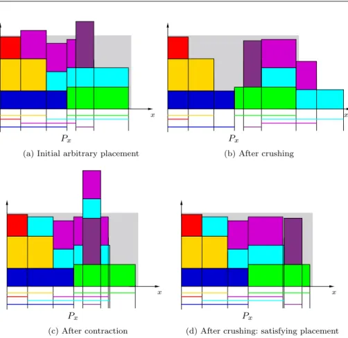
We have developped a local search algorithm to search for satisfying placements Px. Basically, it alternates contraction and crushing phases, modifying step by
step the placement. The process is illustrated in figure 2. The graphic above the intervals of Px shows the occupation of the vertical space: the gray rectangle
is the bin, and for each portion of the x-axis delimited by consecutive interval bounds, a pile consisting of the sections of the items that overlap this portion indicates the height being used. This representation permits to visualize the area that exceeds out of the box. Given an arbitrary but unsatisfying placement Px
x
Px
(a) Initial arbitrary placement
x Px (b) After crushing x Px (c) After contraction x Px
(d) After crushing: satisfying placement
Fig. 2: Searching for a satisfying placement on the x-axis
the intervals of Px are all within the bin width and satisfy the height constraint.
An elementary transformation (a move) consists in removing an interval i from Px,
and re-inserting it at another position. The acceptable destinations for i (that is for its left bound) are 0 and the positions of the left and right bounds of the other intervals in Px. The algorithm starts with a random placement of the intervals such
that each interval is left-supported, that is its left bound is either at the position 0 or at the position of the right bound of another interval. This property may no longer be satisfied. Indeed, it would require that the intervals that loose their support were moved on the left, which may cause other intervals to become unsupported, and so on. The resultant propagation is costly and counterproductive, as it can reduce the available choices for a destination. The contraction and crushing phases have each their own objective.
Contraction. The objective is to have all the intervals within the bin width. Intervals ending beyond W are moved on the left, possibly leading to the violation of the height constraint. As an example, see the transition from the fig. 2b to 2c : The turquoise and pink intervals, which exceed at the right of the bin in fig. 2b, are shifted to the left so as to be in the bin width. The destinations are chosen in such
algorithm search-Px(S, w, h)
in : S a set of items to pack, w, h the width and height of the bin,
phLength is the phase length, maxSteps and nRuns the numbers of steps and runs , 1 for r := 1 to nRuns do
2 Px:= generateRandomPlacement(S, w, h),
3 if width(Px) ≤ w and height(Px) ≤ h then
4 return Px,
5 phase := contract, 6 for s := 1 to maxSteps do
7 if s mod phLength = 0 or phaseCompleted(phase, P x) then
8 phase := switchPhaseMode(phase), (contract ↔ crush) 9 Px:= makeAMove(phase, Px, w, h),
10 if width(Px) ≤ w and height(Px) ≤ h then
11 return Px,
12 end while, 13 end for, 14 return none,
Fig. 3: Function search-Px
a way that if possible, no height exceeding is created, prioritizing the positions that maximize the available free space over the interval. If no such position exists, priority is given to the positions for which the increase in area exceeding above the box is minimal.
Crushing. The objective is to satisfy the height constraint by moving intervals involved in its violation. We have tested many strategies. The best results were obtained by choosing an interval a such that at position lb(a), the position of a left bound, the height constraint is violated before the move, but satisfied after the move. If such intervals exist, the interval for which the amount of free height at the position lb(a) is the smallest after the move is chosen. In the other case, and anyway in 20 per cent of cases, an interval involved in the violation of the height constraint is chosen at random. Eligible destinations are positions that do not cause height constraint violations, giving priority to those for which there is the least free height. Thus the interval can finish beyond the bin width. As an example, see the transition from the fig. 2a to 2b where the turquoise interval (best choice) and the pink interval (random choice) were moved on the right, and the transition from the fig. 2c to 2d.
The algorithm is shown in figure 3. As long as a solution has not been found and within the limit of nRuns runs, each consisting of maxSteps moves, the procedure modifies the placement Px, alternating contraction and crushing phases. A phase
switch is made after a given number of moves or when the objective of the current phase is achieved (lines 7-8). Each run starts with a randomly generated placement (line 2). The function makeAMove consists in choosing an interval and a destination depending on the value of the phase (contract or crush), and in making the move in Px(line 9). If Pxis satisfying the procedure stops and returns Px(line 10).
If no satisfying placement is discovered after nRuns runs the procedure returns none. In our experiments the phase length is set to 10, and the procedure performs two runs of 100,000 moves.
2.2 Searching for Py
Given fixed positions of the items on the x-axis, the problem is to determine if the items can be positioned on the y-axis between 0 and the bin height so that no two items overlap. This problem is similar to a problem of Scheduling With Conflicts [12] with an infinite number of machines, the jobs corresponding to the items, the processing times corresponding to the item heights and the conflict graph being the intersection graph of the intervals in Px. Strong NP-hardness is known to
hold for this problem in the general case. If the processing times are unitary, the decision version of the problem consists in determining whether a given graph G can be partitioned into at most t independent sets of at most k vertices (Partition into Bounded Independent Sets). If G is an interval graph Partition into Bounded Independent Sets remains NP-complete [7].
We have developed a complete search procedure. It is used as an oracle, to confirm that the items can be packed within a given height. Since the positions on the x-axis are already fixed, an exhaustive exploration turns out to be rather efficient, in particular when there is very little free space in the bin. Furthermore, various techniques can be used to reduce the search space.
The function search-Py (figure 4) enumerates all possible ways to pack the
items in the bin with respect to the horizontal positions defined in Px. The items
are packed one after the other, from bottom to top, in such a way that any item which is not at the bottom of the bin is supported by an already packed item (its lower side is in contact with the upper side of its support ). To avoid generating the same packing in different branches, if two items are packed at the same height, the leftmost one in Px must be packed first. Initially, search-Py is called with
parameters (Px, h, S, ∅, π0) where Pxis a placement of the items on the x-axis, h
is the bin height, S is a set containing all the items, and π0 is the initial profile
(a representation of the empty bin). For a sake of simplicity any initial call to search-Py will be contracted to search-Py(S, Px, h) since Py = ∅ and π = π0
parameters are not initially relevant (see figure 8 for such calls).
During the search, the profile π represents the area inside the bin which is no longer available (see fig. 5, the profile is delimited by a green line), and S is the set of items which have still to be packed. If S is not empty, the function explores recursively all the possibilities for the (leftmost) lowest horizontal segment s of the profile π, either putting an item on s (lines 8-11), or removing the area delimited by s (lines 13-15). The items of S which are candidates are those whose interval in Px
is contained in [ls, rs], where lsand rsare the positions of the extremities of s on
the x-axis, and which have a support at s height (line 6, function getCandidates). The leftmost candidates are chosen first, to maximize the chances of finding quickly a solution. Once an item a is placed on the segment s the profile is updated: the area occupied by the item is added to the profile, and also the area between ls
and the position of a left side (see fig. 5a and 5b, the hatched areas). Subsequently putting another candidate at the left of a on the hatched area will not be possible, since it should not be supported. The removal of the space delimited by s simply consists in extending s lowest neighbouring horizontal segment (fig. 5c, the violet line).
Dead-end detection (function heightExceeding). A simple way to verify that there is enough space left in the bin for the items of S consists in comparing at
algorithm search-Py(Px, h, S, Py, π)
in : S the set of the items that have still to be positionned, Pxthe placement of the items on the x-axis,
h the bin height, Pythe positions of the items which are not in S on the y-axis,
π the current profile, 1 if S = ∅ then 2 return Py, 3 if heightExceeding(π, S, Px, h) then 4 return none, 5 s := getLowest(π), 6 C := getCandidates(S, Px, Py, s), 7 for each a ∈ C do 8 π0:= packItem(a, Px, π),
9 p := search-Py(Px, h, S \ {a}, Py· (a, height(s)), π0),
10 if p 6= none then 11 return p, 12 end for, 13 π0:= removeSpace(s, π), 14 if π06= π then 15 return search-Py(Px, h, S, Py, π0), 16 return none,
Fig. 4: Function search-Py
s ls rs a (a) a is lower s ls rs a (b) a is higher rs ls s (c) space removal
Fig. 5: Modification of the profile
each point p of the x-axis, the available free vertical space above the profile with the sum of the heights of the items of S that overlap p. We have implemented a more relevant verification based on the minimal positions of the items on the y-axis. Basically, the minimal position of an item a of S is the maximum height of the profile between a left and right sides (see figure 6). The verification then consists, for a given point p, in positionning the items of S that overlap p one above the other, in order of their minimal positions: the first one is laid on the
b minimal position a b l r h exceeding a minimal position
Fig. 6: Detecting height exceeding
profile or at its minimal position if it is higher, then the next item is laid on top of the first one or at its minimal position if it is higher, and so on. If the last item exceeds the top of the box, there is no way to pack the items that overlap p above the profile and the current branch is abandoned. In practice we consider the intervals delimited by the positions of the sides of the items of S, and apply the verification on each interval. Figure 6 shows an exemple with two items a and b. On the interval [l, r] the sum of the heights of a and b is less than the available vertical space. However, if a and b are positionned one above the other respecting their minimal positions (hatched areas), then a exceeds the top of the bin.
Items miminal positions are updated each time the profile is modified. In case of space removal, the items which were candidates for this space loose their potential supports. For each item a in this case, it must be possible to make a stack with unpacked items laid on a neighbouring segment of s, which could serve as a support for a (see figure 7b). If no such stack exists a could never be packed, and the current branch is a dead end. In the other case a minimal position can be refined to the height of its lowest supporting stack. We implemented a two-phases method to calculate the heights of the supporting stacks, scanning the positions of the sides of the unpacked items in Pxfirst from left to right (figure 7c), then in the reverse
order (figure 7d). The resulting curve (the blue and red lines in figure 7e) represents the minimal height of a supporting stack depending of the position on the x-axis. The minimal position of a given item is the lowest value of the curve between its left and right sides (see figure 7f, the lowest stack supporting a is on the right). Note that minimal positions are also useful to eliminate unsupported items when selecting the candidates for the segment s.
Interchangeable items. If two items a and b are in conflict with exactly the same items in Pxand are in conflict with each other, then packing a and b one on
top of the other or the inverse leads to the same result. We will say that a and b are interchangeable. To avoid the resulting useless explorations it suffices to forbid b to be packed on a if a ≺ b, where ≺ is any a priori total order on the items. This constraint is implemented in searchPy in the following way: each time an item a
is packed, the minimal position of any item b of S which is interchangeable with a and such that a ≺ b is modified, so that b can not be packed on a. In fact, there must exist an item c in S which is not interchangeable with a but is in conflict
s
a
b
(a) a and b are candidates
b
s
a
(b) a stack that supports a
support line
s
(c) calculating from left to right
support line
s
(d) calculating from right to left
b
s
a
(e) final minimal supports
s
a
(f) a minimal position
Fig. 7: Space removal: updating the minimal positions of a and b
with a and b in Px (indeed, if c is interchangeable with a, then c ≺ a and c is also
interchangeable with b but c ≺ b, and then b can not be packed on c). Thus, b minimal position is set to the minimal position of the top of a plus the smallest of the heights of the items of S which are not interchangeable with a but in conflict with a and b in Px. If no such item exists the current exploration is abandoned, else
the new values of the minimal positions are used in the function heightExceeding. The property of interchangeability can be made even stronger. Indeed it suffices to consider the conflicts of a and b which are in S, provided that a and b have the same minimal position. This can be efficiently detected maintaining an ordered list of the bounds of the intervals of Pxcorresponding to items of S. Then a and
b are interchangeable if their left bounds on one hand, and their right bounds on the other hand, are consecutive in the list.
Independent subproblems. During the search, if the set of unpacked items S can be partitioned into two subsets S1 and S2 such that no item of S1 is in
conflict with an item of S2 in Px, then, finding the positions of the items of S1
and finding the positions of the items of S2 are independent subproblems. Each
subproblem can be processed separately: if both are solvable, combining their respective solutions gives a valid placement of the items of S. In the other case the current branch is a dead end. Partitions are detected during the search. Initially the maximal clique decomposition of the interval graph corresponding to Px is
calculated. The intersections of consecutive cliques constitute minimal separators, that is minimal sets of items whose removal disconnects the interval graph. Each
time an item is packed, it suffices to go through its separators searching those that contain only packed items. If there are some, the search is launched consecutively on each independent subproblem.
Stretching Px. Searching for Pyis all the more difficult as there are many overlaps
in Px. Since the items are left-supported in Px, it is possible that, by moving some
items on the right, some overlaps disappear, which gives more chances that a corresponding Py exists. Stretching consists in moving the items one after the
other as much as possible, as long as no new overlap arises, starting with the rightmost items. The same process is then used to stretch Px on the left, so that
the items are left-supported again.
Searching for a solution of a 2OPP instance using search-Px and search-Py
is straightforward. It suffices first to search for a satisfying placement Pxrunning
search-Px, then, if one is found, to verify that it corresponds to a solution of the
instance running search-Py. However this method is not complete, there is no
guarantee to find a solution even if one exists.
3 2D-strip packing problem solving
The 2D-strip packing problem (2SPP) consists in packing a given set of n items into a strip of width W so as to minimize the height (length) of the strip. Many approaches exist for this problem. A simple way to solve a 2SPP instance consists in solving a series of 2OPP instances with different bin heights. Several strategies can be considered: height decrease, height increase, dichotomic search, . . . We propose a new metaheuristic method based on the functions search-Px and search-Px
described in the previous section. It implements a specific strategy that performs back-and-forth movements between the current best height and a minimal bound for the height: periods of progression alternate with periods of verification, the first ones to discover new partial solutions, the later to confirm the existence of valid packings corresponding to these partial solutions. The key point is that the method aims at avoiding working on instances which are unsolvable or of no interest.
The algorithm PVS (progress and verify strategy) (figure 8) is an anytime function which continues searching for better solutions up to a time limit given in parameter. First, a trivial solution is generated running a shelf algorithm, a well known greedy algorithm which consists in placing the items one by one at the same level (height) from the left to the right (as on a library shelf), creating a new level whenever there remains not enough space at the current level for placing the next item. The algorithm returns a pair (Px, Py) which is recorded as the initial solution
in Sol (line 1). PVS computes also a lower bound LB of the optimal height (line 2) from the sum of the items areas and the height of the highest item. Hence, the optimal height belongs to the (possibly large) interval [LB, height(Sol)]. Apart from timeout, finding a solution at height LB is the only stop criterion of PVS (line 3). Lines 3-19 constitute the main part of the algorithm. The objective is to find better solutions progressively, repeating the two following stages:
– Progression (lines 4-10). This stage provides satisfying placements on the x-axis. The function search-Px is called with smaller and smaller values for
algorithm PVS(S, w, limit)
in : S a set of items, w the bin width, out : the solution Sol as a 3-uple (Px, Py, h)
1 Sol := shelfAlgorithm(S, w), 2 LB := computeLowerBound(S, w),
3 while not timeout(limit) and height(Sol) > LB do 4 emptyStack(P), 5 Px:= search-Px(S, w, height(Sol) − 1), 6 while (Px6= none) do 7 push(Px, P), 8 h := placementHeight(Px) − 1, 9 Px:= search-Px(S, w, h), 10 end while,
11 while not isEmpty(P) do 12 Px:= pop(P), 13 Py:= search-Py(S, Px, placementHeight(Px)), 14 if (Py6= none) then 15 Sol := (Px, Py), 16 break, 17 end while,
18 eventually strengthen local search parameters, 19 end while,
20 return Sol,
Fig. 8: Algorithm PVS
the bin height, starting with the height of the solution provided by the shelf algorithm minus one. The process stops as soon as search-Px is not able to
return a placement. Each time a new satisfying placement is found, it is stored in the stack P (line 7), as it may be useful for the other stage, and its effective height is used to fix the height of the bin for the following call of search-Px
(line 8). The effective height, returned by the function placementHeight, is the maximum value of the sums of the heights of the sets of items that intersect each other in Px. The number of runs and the number of modifications per run
allocated to search-Px can be increased before reiterating the two stages, in
order to intensify the search (line 18).
– Verification (lines 11-17). This stage uses the work done in the first stage. The placements stored in P are taken back one after the other, starting with the best ones (that is those with the smallest effective heights), until one that corresponds to a solution is found. The function search-Py is called to make
the verification (line 13). The stage stops either with a better solution (lines 14-16), or when all the placements stored in P have been considered. If there are many items or, at the beginning of the search when the height is not very constraining, the first choices made in search-Py are crucial. Bad decisions
can result in very important computation times and it is not wise to spent too much time searching Py. It is safe then to limit the computation time spent in
search-Py, for example fixing a limit to the number of recursive calls.
Figure 9 illustrates the process on instance gcut13r and on a random instance with 50 items. The x-axis represents the time, the y-axis represents the bin height, and the lines represent the periods during which the functions search-Px (blue
4990 5000 5010 5020 5030 5040 5050 0 10 20 30 40 50 60 fnd Px fail Px search Px fnd Py fail Py search Py 3240 3260 3280 3300 3320 3340 3360 3380 3400 0 10 20 30 40 50 60 fnd Px fail Px fnd Py fail Py TO Py
Fig. 9: PVS solving instance gcut13r and an instance from series O with 50 items
a successful (resp. unsuccessful) call of the functions search-Px and search-Py.
The processing of gcut13r is shown on the left of the figure. search-Pxperformed
10 runs of 100,000 steps, with two additional runs each time the two stages were reiterated. To make the figure clearer, the first iterations are not diplayed (initially the shelf algorithm returned a solution whose height is 5815). Let’s consider the process after 30 seconds of elapsed time: search-Pxis called with the value 5007 as
bin height, but no valid placement Pxis discovered (at 34.2s). Then the progression
stage is reiterated and this time a placement Px with effective height 4999 is
found (at 34.6s). Next call of search-Px with bin height 4998 is unsuccessful.
Then search-Py is run with the placement Px whose effective height is 4999, a
solution is discovered (violet dot at 38.8s at height 4999), and the progression stage is relaunched with bin height 4998. The following calls of search-Px are
unsuccessful, and finally the search stops when the 60 seconds time limit is reached. For the random instance (figure 9 ont the right) the parameters are those that were used for the experimentations (see next section).
4 Experimental results
We have compared PVS with other recent approaches on sets of 2SPP instances. Items orientations are always fixed. Many incomplete approaches for 2SPP are based on greedy algorithms that consist in packing the items one after the other in the bin. They are not much affected by the number of items to pack, and then available instances are often of large size. PVS is not suitable in this case. It is intended to find good quality solutions for hard and relatively small instances, that is instances that are too large for an exact approach to be used. So we have generated such instances.
We have reported the results of GRASP [1], SVC [4], ISA [18], and ISH [23]. The programs SVC, ISA and ISH have been provided to us by the authors, and we are very grateful to them for that. Then PVS, SVC, ISA and ISH have been run in exactly the same conditions, on a machine equipped with a Xeon processor at 2.4 GHz. For GRASP we only reported the best published results that we have found. They were obtained on a machine equipped with a Xeon processor at 2.00 GHz. Each solver was given a computation time of 60 seconds for each instance.
PVS has been run with the same parameters for all the instances. The function search-Pxperforms two runs of 100,000 steps. After performing many experiments
on instances with up to 100 items, it appeared that it wasn’t really worth spending a lot of computation time searching for Py in the verification stage, in
particu-lar when the computation time is limited to 60 seconds. Indeed, if a satisfying placement Py exists, it is generally discovered quickly, since the better choices are
investigated first, and if there is none, the search space can be extremely large, especially when the problem is slightly constrained (that is when the bin height is important). A big effort is required for poor quality solutions, that will probably be improved later. A lazy strategy is more appropriate. So, in all our experiments, search-Py is stopped once 10,000 nodes have been explored. Figure 9 (right)
rep-resents the solving of a random instance with these parameters (random instance with 50 items, search-Py exceeded the 10,000 nodes limit 33 times for 129 calls).
Tables 1 and 2 show the results obtained on series of classical benchmarks. We use instances from Beasley (ngcut and gcut instances) [3], Christophides and Whitlock (cgcut instances) [10], Bengston (beng instances) [5], Berkey and Wang (Class01-Class06) [6], and Martello and Vigo (Class07-Class10) [21]. Each program was run 40 times on each instance, except SVC whose results do not depend on a random number generator. For the others, we reported the averages of the results obtained for each instance. We have also reported the number n of items, the width w of the strip, and the thickness and widthness of the solutions returned by PVS. Roughly, the thickness represents the average number of layers. It is calculated as follows: for each item i, we calculate anlo(i), the average number of layers over i, which is either 1 if there is no item over i, or one plus the average of the anlo values of the items that are immediately over i (that is which are not necessarily in contact with i but such that there is no item between them). The thickness is the average value of the anlo values of the items which are at the bottom of the bin. The widthness is calculated in the same manner in the other dimension. Columns thkn. and wdth. contain the average thickness and widthness.
On small instances all solvers have fairly comparable results, and for very small instances all the solvers discover optimal solutions, see for example the series ngcut. When the number of items is important PVS is strongly penalized, as can be seen with beng and Class01-Class10 instances when there are more then 80 items. However, if we consider some particular instances which seem to be hard because the results of the different approaches are rather disparate, ISA, ISH and PVS are the more efficient. This is the case of instances gcut04, gcut08, gcut13 and gcut13r. Specially on gcut13, PVS provides very good results. We have noticed that these instances admit few solutions of very good quality. It is worth to note that increasing the computation time allows for better results, but we did not observe any change in the hierarchy.
Berkey and Wang, and later Martello and Vigo developped classes of instances using specific parameters. In each class items sizes are chosen in given ranges. For example, in Class07, 70 per cent of the items have their height and width chosen at random uniformly in [1, 50] × [66, 100]. It is clear that PVS performance is correlated to the widthness of the solutions (see table 2). If the widthness is small PVS performs better than the other approaches, as in Class05 or Class08. In the other case, in Class04 or Class06 for example, PVS is less efficient, even more when there are many items. We wanted to analyse more precisely the performances of PVS according to the shape of the items and the characteristics of the solutions. Indeed, PVS operates in a very different manner compared to SVC, ISA and ISH. These ones fill the strip from the bottom, using heuristics to choose one or several
Instance
Name n w thkn. wdth. GRASP SVC ISA ISH PVS ngcut01 10 10 3.9 1.8 23 23 23 23 23 ngcut02 17 10 6.5 2.3 30 30 31 30 30 ngcut03 21 10 6.1 3.4 28 28 28 28 28 ngcut04 7 10 1.3 2.8 20 20 20 20 20 ngcut05 14 10 3.5 3.2 36 36 36 36 36 ngcut06 15 10 5.6 2.3 31 31 31 31 31 ngcut07 8 10 1.1 3.4 20 20 20 20 20 ngcut08 13 20 2.6 3.5 33 34 34 34 33 ngcut09 18 20 5.2 3.2 50 51 51 50 50 ngcut10 13 20 4 2.8 80 80 80 80 80 ngcut11 15 30 4.3 3.3 52 52 52 52 52 ngcut12 22 30 8.8 2.3 87 87 87 87 87 cgcut1 16 10 4.6 2.8 23 23 23 23 23 cgcut2 23 70 4.4 4.8 65 65 65 65 64.5 cgcut3 62 70 22.9 2.3 661 661 662 659.5 660.5 gcut01 10 250 9 1 1,016 1,016 1,016 1,016 1,016 gcut02 20 250 7.5 1.9 1,191 1,187 1,187 1,187 1,187 gcut03 30 250 11.7 1.7 1,803 1,803 1,803 1,803 1,803 gcut04 50 250 23.3 2 3,002 3,016 3,002 3,004.7 3,001.4 gcut05 10 500 3.4 2 1,273 1,273 1,273 1,273 1,273 gcut06 20 500 7.3 1.9 2,627 2,632 2,627.8 2,622 2,622 gcut07 30 500 13.3 1.6 4,693 4,693 4,693 4,693 4,693 gcut08 50 500 23 2.1 5,912 5,876 5,880.4 5,869.4 5,862.8 gcut09 10 1,000 3.7 1.5 2,317 2,317 2,317 2,317 2,317 gcut10 20 1,000 7.7 1.8 5,964 5,973 5,964 5,964 5,964 gcut11 30 1,000 11.3 2 6,899 6,891 6,877.9 6,868.5 6,866.5 gcut12 50 1,000 20.2 1.7 14,690 14,690 14,690 14,690 14,690 gcut13 32 3,000 8.3 3.8 4,994 4,977 4,956.7 4,968.6 4,916.2 gcut09r 10 1,000 3.1 1.9 2,256 2,261 2,241 2,241 2,241 gcut10r 20 1,000 8.2 1.6 6,393 6,393 6,393 6,393 6,393 gcut11r 30 1,000 10.4 1.7 7,736 7,736 7,736 7,736 7,736 gcut12r 50 1,000 20.1 1.9 13,172 13,172 13,172 13,172 13,172 gcut13r 32 3,000 6.2 4.9 5,009 5,035 5,001.2 5,026.6 5,005.6 beng01 20 25 3.9 5 30 30 31 30.8 30 beng02 40 25 7.7 5 57 57 57 57 57.1 beng03 60 25 11.7 5.1 84 84 84 84 84.1 beng04 80 25 14.8 5.3 107 107 107 107 108 beng05 100 25 18.7 5.3 134 134 134 134 135.2 beng06 40 40 4.9 8.1 36 36 36 36 36 beng07 80 40 9.2 8.5 67 67 67 67 68.7 beng08 120 40 14.2 8 101 101 101 101 107.9 beng09 160 40 19 8 126 126 126 126 139.8 beng10 200 40 22.9 8 156 156 156 156 170.9
Table 1: Computational results on instances from Beasley, Christophides and Whitlock, and Bengston.
items to be packed in the lowest gap. These heuristics take as input an ordered sequence of items and rely on scoring rules, or, in the case of SVC, use a knapsack algorithm to select the items to be placed in the gap, where profits (pseudo-profits) are associated to the items to favor the selection of items that seem hard to pack. PVS handles the two dimensions of the space differently, and the functions search-Px and search-Py work in very different ways. As a result, the
width-to-height ratios of the items, the diversity in items sizes, and the strip width, which determines the thickness, have a significant effect on the performances. Thus we have generated instances in which the sizes but also the areas of the items are chosen in fixed ranges.
Instance
Name n w thkn. wdth. GRASP SVC ISA ISH PVS
Class01 20 10 10.6 1.9 61.3 61.4 61.3 61.2 61.2 40 10 21.9 1.8 121.9 121.9 121.8 121.8 121.8 60 10 33.8 1.8 188.7 188.5 188.6 188.5 188.5 80 10 47.2 1.7 262.9 262.6 262.6 262.6 262.6 100 10 55.2 1.8 305.6 304.8 304.9 304.8 304.8 Class02 20 30 3.5 5.7 19.8 19.8 19.8 19.8 19.8 40 30 7.1 5.7 39.1 39.1 39.1 39.1 39.1 60 30 11 5.4 60.2 60.1 60.1 60.1 60.6 80 30 15.2 5.2 83.2 83.2 83.2 83.2 83.6 100 30 18.4 5.4 100.5 100.5 100.5 100.5 101.7 Class03 20 40 8.5 2.3 163.5 164.8 163.7 162.8 162.4 40 40 18 2.2 333.8 333.9 333.3 332.9 332.4 60 40 27.4 2.2 506.6 506.8 505.5 504.9 504.9 80 40 38.4 2.1 710 709.8 709.2 708.8 708.7 100 40 45.5 2.2 840.2 839.5 838 836.8 837.3 Class04 20 100 3.4 5.9 63.4 63.8 63.4 63.3 62.9 40 100 6.9 5.8 126.3 125.8 125.5 125.3 126.7 60 100 10.8 5.4 196.7 195.3 195.1 194.5 199.9 80 100 15.2 5.1 272.2 270.2 269.8 268.8 282.7 100 100 18.6 5.2 327.3 325.2 324.4 323.3 354 Class05 20 100 9.5 2 533.9 537.1 533.9 534.1 533.5 40 100 19.7 2 1,074.7 1,076.5 1,073.5 1,073.2 1,072.4 60 100 31.7 1.9 1,645.9 1,647.3 1,643.2 1,642.1 1,640.5 80 100 44.3 1.8 2,290.4 2,288.7 2,288.9 2,287.9 2,286.2 100 100 51.2 2 2,652 2,652.2 2,645.4 2,643.7 2,641 Class06 20 300 3.2 6.3 167.3 169.5 167.6 167.7 166.6 40 300 6.4 6.2 333.6 332 332.3 332.2 334.1 60 300 10 5.8 520.6 515.9 517.6 515.8 528.9 80 300 14.2 5.4 718.9 713.8 714.6 712.4 750.8 100 300 17.3 5.5 865.4 859.8 860 857.1 935.2 Class07 20 100 14.3 1.3 501.9 501.9 501.9 501.9 501.9 40 100 28.8 1.3 1,059 1,059.9 1,059.4 1,059 1,059 60 100 44.9 1.3 1,529.6 1,530 1,529.6 1,529.6 1,529.6 80 100 62.2 1.3 2,222.2 2,222.1 2,222.1 2,222.1 2,222.1 100 100 77.9 1.3 2,645.2 2,644 2,644 2,643.9 2,643.9 Class08 20 100 6.5 3.1 458 461.1 456.5 456.2 453.3 40 100 14.1 2.8 954.4 955.5 949.3 946.7 940.4 60 100 20.3 3 1,405.9 1,400.8 1,398.6 1,391.5 1,389 80 100 28.5 2.8 1,973.6 1,961.9 1,956.4 1,948.5 1,953.4 100 100 35.7 2.8 2,439.5 2,419.8 2,412.1 2,403 2,460.9 Class09 20 100 15.3 1.3 1,106.8 1,106.8 1,106.8 1,106.8 1,106.8 40 100 31.8 1.3 2,190.6 2,190.7 2,191.1 2,190.6 2,190.6 60 100 48.5 1.2 3,410.4 3,410.4 3,410.4 3,410.4 3,410.4 80 100 65.8 1.2 4,588.1 4,588.1 4,588.1 4,588.1 4,588.1 100 100 78.4 1.2 5,434.9 5,434.9 5,434.9 5,434.9 5,434.9 Class10 20 100 7.8 2.5 350.5 350.9 349.5 349.5 349.3 40 100 16.3 2.4 664.5 666.8 662.8 661.3 659.1 60 100 23.3 2.5 935.5 936.3 932.9 930 929.3 80 100 31 2.5 1,209.7 1,210.9 1,204 1,200.1 1,202.5 100 100 38.5 2.5 1,515.1 1,512.1 1,504.6 1,499.2 1,521.4
Table 2: Computational results on Berkey and Wang instances (Class01-Class06) and Martello and Vigo instances (Class07-Class10).
(a) strip width = 4000
(b) strip width = 6000
(c) strip width = 10000
(d) strip width = 8000
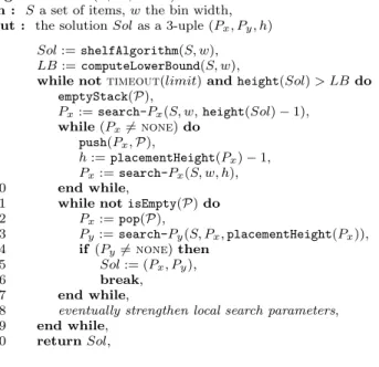
Fig. 10: Solutions returned by PVS for random instances with 60 items and various strip widths
First, we did tests on instances of various sizes varying the strip width. Table3 shows some results on instances with 30, 40, 50, 60, 70 and 80 items. For each series we have generated 10 instances, with fairly similar rectangles of large di-mensions. Thus, the solutions are rather fragmented (there is wasted space almost everywhere), and there are many good solutions. Items widths and heights are chosen at random between 400 and 1000. Furthermore items whose area is not in the range 350000−400000 are rejected (see fig. 10 for some examples). We have chosen the strip widths so that there are no trivial solutions. Each line in table 3 shows the results obtained with the 10 instances of n items and a given strip width. ISA, ISH and PVS have been run 40 times for each instance. Results are given in terms of mean height over the 10 instances, and average best height (that is the average of the best results of the 10 instances). For SVC, ISA and ISH we just reported the loss or gain in percentage compared to PVS (a positive value corresponds to worse solutions). We indicated the average results of each series, although these are of little significance.
As with classical instances it is clear that the more items there are, the less PVS is efficient compared to the other approaches. Indeed in this case, finding Py
is all the more difficult, and very often the search is abandoned. Thus, although the progression stage provides many good quality placements, none of them gives a solution. The performances of the different approaches also vary significantly with the strip width. Depending on the strip proportions (many layers or few layers) one or another is more appropriate. PVS is rather better when the thickness of the solutions is low. In fact SVC, ISA and ISH heuristics do not take into consideration the difficulty of filling the free area above the current packing with the remaining items. A bad choice can have important consequences, especially when there is little space left above, which is all the more the case when the thickness is low.
Instances PVS SVC ISA ISH n w thkn. wdth. mean best mean % mean % best % mean % best % 30 2000 9.7 3.1 5839.5 5815.7 −0.07 −0.02 0 0.32 0.23 30 3000 6.5 4.7 3899.2 3878.1 0.3 0.09 0.01 0.49 0.28 30 4000 4.8 6.3 2929.7 2913.9 0.86 0.85 0.54 1.12 0.65 30 6000 3.2 9.4 1956.6 1943.4 3.56 3.26 2.66 2.56 2.14 30 8000 2.4 12.7 1503.4 1499.4 4.01 3.13 1.89 2.66 1.53 30 10 000 1.9 16.1 1282.9 1278.7 1.46 2.03 1.17 0.34 0.13 30 12 000 1.5 19.3 1137 1130.9 −0.85 −0.06 0.04 −0.87 −0.34 30 15 000 1.3 23.7 970.8 970.8 0 0 0 0 0 1.16 1.16 0.79 0.83 0.58 40 2000 12.5 3.2 7782.4 7757.1 −0.22 −0.1 −0.2 0.01 −0.08 40 3000 8.3 4.8 5215.9 5192.5 −0.35 −0.14 −0.33 0.19 −0.18 40 4000 6.2 6.4 3924.2 3903.4 −0.01 0.25 0 0.78 0.46 40 6000 4.1 9.7 2619.7 2605.5 2.31 1.88 1.3 1.68 1.24 40 8000 3.1 13 1970.7 1960 4.59 4.08 3.58 2.02 1.37 40 10 000 2.4 16.3 1624.5 1617.9 4.08 2.7 1.91 2.31 1.9 40 12 000 2 19.8 1353.2 1347.3 2.18 4.77 3.96 1.23 0.91 40 15 000 1.6 25 1212.4 1206 −0.82 0.7 0.85 −1.22 −0.75 40 20 000 1.2 32.9 974.5 974.5 0 0 0 0 0 1.31 1.57 1.23 0.78 0.54 50 2000 16 3.2 9710.5 9677 −0.53 −0.17 −0.45 −0.2 −0.3 50 3000 10.7 4.7 6517.3 6489 −0.84 −0.41 −0.66 −0.2 −0.52 50 4000 8.1 6.2 4911 4885.9 −0.84 −0.21 −0.46 0.2 −0.04 50 6000 5.3 9.4 3279.6 3262.7 0.69 1.12 0.72 1.49 1.02 50 8000 4 12.6 2459.7 2445.7 3.09 2.79 2.26 1.82 0.79 50 10 000 3.2 15.7 1971.7 1962 5.08 4.88 3.92 3.69 2.85 50 12 000 2.6 19.1 1679.8 1672.3 4.29 4.19 3.5 1.85 1.54 50 15 000 2.1 23.9 1360 1354.4 2.29 5.58 4.63 1.9 1.51 50 20 000 1.5 32.4 1146.5 1132.7 −2.46 −0.24 0.59 −2.51 −1.32 1.2 1.95 1.56 0.89 0.61 60 2000 18.8 3.2 11 667.7 11 629.9 −0.54 −0.29 −0.45 −0.19 −0.33 60 3000 12.6 4.8 7853 7811.5 −1.28 −0.75 −0.93 −0.58 −0.61 60 4000 9.5 6.3 5926.6 5887.8 −1.24 −0.76 −0.91 −0.45 −0.56 60 6000 6.3 9.5 3959.5 3937.4 0.1 0.44 0.14 0.86 0.56 60 8000 4.7 12.8 2966.8 2952.2 1.68 2.04 1.69 1.23 1.08 60 10 000 3.7 16.1 2371.1 2358.3 3.68 3.18 2.65 0.74 0.61 60 12 000 3.1 19.3 1983.4 1970.7 5.32 4.55 4.46 2.9 1.84 60 15 000 2.5 24.3 1632 1623 4.47 3.95 3.19 2.44 2.19 60 20 000 1.8 33 1290.5 1285.5 1.54 3.34 3.2 −0.06 −0.31 1.53 1.74 1.45 0.77 0.5 70 2000 21.7 3.3 13 596.1 13 545.2 −0.89 −0.4 −0.44 −0.39 −0.41 70 3000 14.6 4.8 9196.7 9114.7 −2.01 −1.47 −1.17 −1.31 −0.95 70 4000 10.9 6.4 6958.3 6877.4 −2.39 −1.78 −1.29 −1.46 −0.96 70 6000 7.3 9.6 4647.3 4598.6 −1.11 −0.69 −0.41 −0.34 −0.16 70 8000 5.4 12.8 3471.9 3450.8 0.84 0.81 0.49 1 0.76 70 10 000 4.3 16.2 2771 2758.2 2.27 2.44 1.99 2.27 1.78 70 12 000 3.6 19.5 2307.3 2297.7 3.45 3.42 3.13 1.66 1.64 70 15 000 2.9 24.4 1852.4 1842.6 5.3 4.39 4.69 −0.03 −0.51 70 20 000 2.2 32.7 1401.5 1393.2 5.59 8.63 8.53 5.76 4.59 1.23 1.71 1.72 0.8 0.64 80 2000 25.1 3.2 15 542.7 15 486.6 −1 −0.51 −0.67 −0.53 −0.59 80 3000 16.9 4.7 10 583.2 10 454.3 −2.8 −2.2 −1.54 −2.18 −1.5 80 4000 12.7 6.2 8035.1 7886 −3.34 −2.91 −1.65 −2.62 −1.4 80 6000 8.5 9.3 5388.4 5290.6 −2.94 −2.33 −1.33 −1.86 −0.74 80 8000 6.3 12.6 4017.3 3959.7 −1.1 −0.73 0.13 −0.28 0.29 80 10 000 5 15.9 3187.3 3162.2 1.02 1.28 1.36 0.83 0.35 80 12 000 4.2 19.1 2649.9 2634.6 2.57 2.38 2.4 2.72 2.07 80 15 000 3.3 24 2123.1 2110.7 4.4 4.31 4.35 4.12 3.9 80 20 000 2.5 32.2 1634.3 1627.2 4.39 4.27 3.9 2.08 2.02 0.13 0.4 0.77 0.25 0.49
(a) type A, w = 4000 (b) type B, w = 4000
(c) type C, w = 8000
(d) type A,B,C, w = 6000
(e) type D, w = 6000 (f) type E, w = 6000
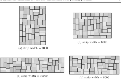
Fig. 11: Solutions of instances with 50 items of specific types
In this case the hardest part for PVS is to find good placements on the x-axis, and search-Pxseems efficient for that. On the contrary, when the strip is narrow
the chances of finding a solution given a placement Px are pretty low. Indeed
Py’s search space is then very large, and the search is often unsuccessful. Finally,
when the strip is extremely wide (for example 50 items with strip width 20000, the thickness is 1.5) SVC, ISA and ISH especially are better than PVS. In this particular situation the solutions are composed of stacks of one or two items and PVS progression stage is struggling at producing placements of good quality.
Depending on the shapes of the items PVS is more or less effective. We gener-ated instances with items of specific types, considering the following categories: A squares: width and height are between 450 and 550,
B 2-rectangles: width between 450 and 550, height between 900 and 1000, rotated with probability 0.5,
C 5-rectangles: width between 450 and 550, height between 2300 and 2600, rotated with probability 0.5,
D unconstrained : width and height are between 450 and 1000,
E same areas: width between 400 and 1000, height unconstrained, area between 350,000 and 400,000, rotated with a probability of 0.5, width-to-height ratios are equally distributed (between 1 and 2.5 if we consider the largest dimension over the smallest).
Table 4 shows the results of experimentations on sets of instances constructed with items from one or several categories1(see figure 11 for some examples). Each set contains 10 instances of 50 items. Items are chosen at random in the categories attached to the set with the same probability. We compared SVC, ISA, ISH and PVS on each set, with various strip widths. Except SVC, each solver has been run 20 times on each instance, then we reported for each set and each width the average result and the average of the best results of the 10 instances. Results are displayed as a percentage of gain or loss compared to PVS.
The results of SVC, ISA, ISH and PVS are very close (there is an exception with SVC in series C, in which the items are long rectangles with fairly similar dimen-sions). However PVS finds generally better solutions than the other approaches, especially when the strip is wide, for the same reasons as mentioned above. This is particularly the case when the items have very varied shapes, as in the series D and E. These instances are rather hard: the items are not easily interchangeable as in the other series, and there is wasted space in many places (see figure 11e and 11f). Compared to the other series, the density in the solutions is high (the bin is better filled) and the items are strongly imbricated with each other. This suggests that there is very little similarity between two good quality solutions. We also observe running PVS that satisfying placements on the x-axis give rarely a solution.
5 Conclusion
We have presente a new metaheuristic approach, called PVS, for the strip packing problem in a two-dimensional space. It consists of alternately performing pro-gression phases and verification phases, discovering solutions of higher and higher quality, until a given time limit is reached. The progression phase focuses on solving relaxations of the problem, using a local search procedure that returns satisfying positions of the items on the x-axis. The verification phase determines whether the partial solutions resulting from the progression phase can be extended to com-plete solutions, calling an exact procedure that searches for compatible positions of the items on the y-axis. To avoid situations where the search for the positions on the y-axis does not terminate, the exact procedure may be interrupted after a given number of steps. Experimentations on classical benchmarks and on ran-domly generated instances show the usefulness of PVS with middle size instances, a category for which exact approaches are not applicable and metaheuristics are not necessarily efficient. PVS gives particularly good results when the shapes of the items are varied but fairly similar. In this case the instances are difficult in the sense that the items are not interchangeable and strongly imbricated the ones with the others, and then finding a good solution requires a global arrangement.
We plan to adapt the approach for the two-dimensional knapsack problem and to implement the rotation of the items. The idea could also be applied to packing problems in a three-dimensional space. The progression phase would then consist in fixing the positions of the items in the plane, while items elevations would be calculated in the verification phase. These problems can be very hard even when there are few items and our approach is appropriate for such cases.
1 Instances are available at
http://www.dil.univ-mrs.fr/~gcolas/packing/ random-instances.tgz.
Items Instances PVS SVC ISA ISH seriesshape n w thkn. wdth. mean best mean% mean% best % mean% best %
50 1000 26.4 1.8 13 831 13 831 0 0.01 0.01 0 0 width: 50 2000 12.5 3.8 6456.1 6437 0.08 −0.08 −0.06 0.16 0.17 450 − 550 50 3000 8.3 5.7 4353.8 4337.7 0.87 0.71 0.7 0.86 0.83 50 4000 6.2 7.5 3336.4 3319.3 1.37 1.16 1.24 1.37 1.45 A 50 6000 4.1 11.2 2342.7 2332.9 1.4 1.4 1.28 1.58 1.5 50 8000 3.1 14.9 1858.8 1851.8 1.17 0.96 0.95 1.01 0.92 height: 50 10 000 2.6 19 1460.9 1458.4 1.08 0.45 0.4 0.25 0.25 450 − 550 50 12 000 2.1 22.6 1382.5 1378.5 0.29 0.23 0.3 0 0.09 0.78 0.6 0.6 0.66 0.65 50 2000 17.6 2.8 12 240 12 234 0.09 0.01 0.02 −0.02 −0.01 width: 50 3000 11.6 4.2 8170.2 8163.4 0.19 0.03 0.04 0.01 0.03 450 − 550 50 4000 8.8 5.6 6157.4 6137.5 0.56 0.17 0.26 0.17 0.29 50 6000 6 8.4 4190.1 4177 1.23 0.7 0.6 0.84 0.79 B 50 8000 4.5 11.2 3230.2 3220.9 1.3 0.81 0.6 0.86 0.75 50 10 000 3.6 13.8 2453.6 2449.8 1.17 0.85 0.67 0.4 0.31 height: 50 12 000 3 16.6 2286 2281.8 0.99 0.72 0.57 0.02 0.13 900 − 1000 50 15 000 2.4 21.2 1861.5 1858.5 1.21 0.95 0.86 0.57 0.41 0.84 0.53 0.45 0.36 0.34 50 3000 21.9 2.3 21 766.1 21 740.8 5.01 0.41 0.32 0.44 0.3 width: 50 4000 14 4 16 146.3 16 110.2 0.63 0.4 0.3 0.39 0.29 450 − 550 50 6000 9.9 5.6 10 727.7 10 688.3 2.31 −0.05 −0.13 0.33 0.25 50 8000 7.9 7.3 8045.1 8012.1 2.11 0.13 0.13 0.4 0.38 C 50 10 000 6.8 9.2 6510.5 6481.4 0.47 0.18 0.2 0.16 0.2 50 12 000 5.2 11.7 5425.2 5401.9 0.4 0.24 0.35 0.06 0.12 height: 50 15 000 4.7 12.8 4428 4412.9 1.27 1.08 1.13 0.24 0.29 2300 − 2600 50 20 000 3.2 18.7 3384.3 3372.8 0.43 1.5 1.65 0.41 0.41 1.58 0.49 0.49 0.3 0.28 50 3000 14.4 3.5 11 260 11 232.3 0.3 0.29 0.14 0.44 0.28 50 4000 10.6 4.8 8436 8401.1 −0.13 0.32 0.3 0.5 0.58 50 6000 7.2 7.1 5668.2 5642 0.07 0.14 0.13 0.15 0.24 50 8000 5.3 9.5 4264.1 4245.7 0.04 0.22 0.31 0.14 0.23 mix A, B, C 50 10 000 4.1 12.5 3464.3 3451 0.38 0.4 0.39 0.37 0.22 50 12 000 3.3 15.4 2931.2 2920.4 0.35 0.43 0.42 0.31 0.43 50 15 000 2.4 19.1 2576 2576 0 0 0 0 0 50 20 000 1.9 22.3 2576 2576 0 0 0 0 0 0.13 0.22 0.21 0.24 0.25 50 2000 18.2 2.7 13 654.5 13 613.1 −0.27 −0.5 −0.42 −0.42 −0.33 width: 50 3000 11.9 4 9006.4 8976.8 −0.3 −0.69 −0.69 −0.22 −0.29 450 − 1000 50 4000 9 5.3 6787.2 6766 −0.89 −0.84 −0.93 −0.02 −0.22 50 6000 6 7.9 4545.8 4528.5 −0.35 −0.42 −0.54 0.04 −0.21 D 50 8000 4.5 10.5 3416.4 3401.7 0.33 0.52 0.34 0.98 0.83 50 10 000 3.6 13.1 2739.9 2728.5 1.27 1.53 1.32 1.52 1.33 height: 50 12 000 3 15.8 2287.4 2278.2 1.39 1.47 1.33 0.78 0.63 450 − 1000 50 15 000 2.4 19.8 1861.4 1851.1 4.07 3.59 3.03 3.99 3.81 50 20 000 1.9 26.2 1471.4 1466.6 1.71 1.2 1.2 −0.75 −0.48 0.77 0.65 0.52 0.66 0.56 50 2000 16.1 3.2 9704.6 9668 −0.49 −0.24 −0.45 −0.09 −0.07 width: 50 3000 10.8 4.7 6520.7 6497.2 −0.82 −0.57 −0.69 −0.27 −0.45 400 − 1000 50 4000 8 6.2 4914.1 4892.3 −0.6 −0.34 −0.56 0.28 −0.02 50 6000 5.3 9.4 3280.8 3266.2 0.76 1.19 0.81 1.58 1.23 E height: – 50 8000 4 12.6 2461.4 2449.1 2.85 2.74 2.48 1.52 1.16 50 10 000 3.2 15.8 1973.7 1965.1 4.72 4.72 4.24 3.8 3.16 area: 50 12 000 2.6 19.2 1668.8 1662.4 4.17 4.54 3.7 1.77 1.68 350K-400K 50 15 000 2.1 24.1 1353.2 1348.9 2.34 6.32 5.14 2.34 2.06 50 20 000 1.5 32.5 1150.2 1142.6 −2.06 −0.28 0.31 −2.06 −1.41 1.21 2.01 1.66 0.99 0.82
Table 4: Computational results on randomly generated instances with various items shapes.
References
1. Alvarez-Valdes, R., Parre˜no, F., Tamarit, J.: Reactive grasp for the strip-packing problem. Computers & Operations Research 35(4), 1065 – 1083 (2008). DOI 10.1016/j.cor.2006.07. 004
2. Baker, B., Coffman, E., Rivest, R.: Orthogonal packing in two dimensions. SIAM J. of Computing 9(4), 846–855 (1980)
3. Beasley, J.E.: Algorithms for unconstrained two-dimensional guillotine cutting. The Jour-nal of the OperatioJour-nal Research Society 36(4), 297–306 (1985)
4. Belov, G., Scheithauer, G., Mukhacheva, E.A.: One-dimensional heuristics adapted for twodimensional rectangular strip packing. Journal of the Operational Research Society pp. 823–832 (2008)
5. Bengtsson, B.: Packing rectangular pieces - a heuristic approach. Comput. J. 25(3), 353– 357 (1982)
6. Berkey, J.O., Wang, P.Y.: Two-dimensional finite bin-packing algorithms. Journal of the Operational Research Society 38(5), 423–429 (1987). URL https://doi.org/10.1057/ jors.1987.70
7. Bodlaender, H.L., Jansen, K.: Restrictions of graph partition problems. part i. Theor. Comput. Sci. 148(1), 93–109 (1995). DOI 10.1016/0304-3975(95)00057-4
8. Burke, E.K., Kendall, G., Whitwell, G.: A new placement heuristic for the orthogonal stock-cutting problem. Oper. Res. 52(4), 655–671 (2004). DOI 10.1287/opre.1040.0109 9. Chazelle, B.: The bottom-left bin-packing heuristic: An efficient implementation. IEEE
Transactions on Computers 32(8), 697–707 (1983)
10. Christofides, N., Whitlock, C.: An Algorithm for Two-Dimensional Cutting Problems. Operations Research 25(1), 30–44 (1977). DOI 10.1287/opre.25.1.30
11. Clautiaux, F., Carlier, J., Moukrim, A.: A new exact method for the two-dimensional orthogonal packing problem. European Journal of Operational Research 183(3), 1196– 1211 (2007)
12. Even, G., Halld´orsson, M.M., Kaplan, L., Ron, D.: Scheduling with conflicts: online and offline algorithms. Journal of Scheduling 12(2), 199–224 (2009). DOI 10.1007/ s10951-008-0089-1
13. Fekete, S.P., Schepers, J.: A combinatorial characterization of higher-dimensional orthog-onal packing. Mathematics of Operations Research 29(2), 353–368 (2004)
14. Garey, M.R., Johnson, D.S.: Computers and Intractability; A Guide to the Theory of NP-Completeness. W. H. Freeman & Co., New York, NY, USA (1979)
15. Grandcolas, S., Pinto, C.: A new search procedure for the two-dimensional orthogonal packing problem. J. Math. Model. Algorithms in OR 14(3), 343–361 (2015). DOI 10. 1007/s10852-015-9278-z
16. Iori, M., Martello, S., Monaci, M.: Optimization and Industry: New Frontiers, chap. Meta-heuristic Algorithms for the Strip Packing Problem, pp. 159–179. Springer US, Boston, MA (2003). DOI 10.1007/978-1-4613-0233-9\ 7
17. Lesh, N., Marks, J., McMahon, A., Mitzenmacher, M.: New heuristic and interactive approaches to 2d rectangular strip packing. J. Exp. Algorithmics 10 (2005). DOI 10.1145/1064546.1083322
18. Leung, S.C.H., Zhang, D., Sim, K.M.: A stage intelligent search algorithm for the two-dimensional strip packing problem. European Journal of Operational Research 215(1), 57–69 (2011). DOI 10.1016/j.ejor.2011.06.002
19. Lodi, A., Martello, S., Monaci, M.: Two-dimensional packing problems: A survey. Euro-pean Journal of Operational Research 141(2), 241–252 (2002)
20. Martello, S., Monaci, M., Vigo, D.: An exact approach to the strip-packing problem. Journal on Computing 15(3), 310–319 (2003)
21. Martello, S., Vigo, D.: Exact solution of the two-dimensional finite bin packing prob-lem. Management Science 44(3), 388–399 (1998). URL http://www.jstor.org/stable/ 2634676
22. Neveu, B., Trombettoni, G., Araya, I., Riff, M.: A strip packing solving method using an incremental move based on maximal holes. International Journal on Artificial Intelligence Tools 17(5), 881–901 (2008). DOI 10.1142/S0218213008004205
23. Wei, L., Hu, Q., Leung, S.C., Zhang, N.: An improved skyline based heuristic for the 2d strip packing problem and its efficient implementation. Computers & Operations Research 80, 113 – 127 (2017). DOI https://doi.org/10.1016/j.cor.2016.11.024