Drag amplification and fatigue damage in vortex-induced vibrations

Drag Amplification and Fatigue Damage

in Vortex-Induced Vibrations

by

Vikas Gopal Jhingran

Submitted to the Department of Mechanical Engineering

in partial fulfillment of the requirements for the degree of

Doctor of Philosophy in Ocean Engineering

at the

MASSACHUSETTS INSTITUTE OF TECHNOLOGY

[3o,,e 00O3

April 2008

© Massachusetts Institute of Technology 2008. All rights reserved

t / % SI

A uthor

... ... . ... ...

...

Department of Mechanical Engineering

April 24, 2008

C ertified by

... ...

J. Kim Vandiver

Professor of Mechanical and Ocean Engineering, MIT

Thesis Supervisor

Accepted by

...

...

Lallit Anand

Chairman, Department Committee on Graduate Students

LkSETTS INST1T E ECHNOLOGY

2

9

2008

LIBRARIES

MtCHVgg

JUL

Drag Amplification and Fatigue Damage

in Vortex-Induced Vibrations

by

Vikas Gopal Jhingran

ABSTRACT

Fatigue damage and drag force amplification due to Vortex-Induced-Vibrations (VIV) continue to cause significant problems in the design of structures which operate in ocean current environments. These problems are magnified by the uncertainty in VIV prediction, particularly with regard to fatigue damage. Although the last fifteen years has seen significant advancement in VIV prediction, important fatigue and drag related questions remain unanswered.

This research addresses two important problems. The first is the difficulty in measuring local drag coefficients on long flexible cylinders, excited by VIV. At best engineers are forced to use spatially averaged drag coefficients. This is especially inaccurate when the pipe and flow properties change, either due to partial coverage with VIV mitigation devices, such as strakes or fairings, or shear in the incident current profile. The second problem is the lack of design procedures that account for the effect on fatigue damage due to the higher harmonics in the VIV strain response.

To address these problems, two experiments were performed to collect data, the first in October of 2004 and the second in October of 2006. Both of these experiments were designed specifically to collect strain measurements from a densely instrumented pipe undergoing VIV at high mode numbers when subjected to current profiles with varying amounts of shear.

Data from these experiments was used to develop a method to extract local drag forces from the measured mean strain. This method, when applied to a partially faired pipe undergoing VIV, successfully and accurately distinguished the dissimilar local drag coefficient between the bare pipe region and the region with fairings. In bare pipes, for the first time the method allowed for the measurement of the variation of local drag coefficient along the length of a flexible pipe undergoing VIV in sheared current.

Further by using filtering techniques, the higher harmonics were isolated and analyzed, particularly for their magnitude and phase response characteristics. Interesting features about the phase relationships between the first, second and third harmonics were observed when the primary VIV response was in the form of a traveling wave. Finally, data revealed some inaccuracies in the fatigue estimation techniques currently being used by the oil and gas industry. Two methods are suggested to incorporate the higher harmonics in VIV related fatigue design while correcting the observed inaccuracies in the current methods.

The results revealed limitations in the commonly used, vibration-amplitude based methods of calculating local drag coefficients and may lead to modifications to correct these limitations. These findings also provide tools for researchers to include the higher harmonics in VIV related fatigue damage calculations and remove some of the uncertainty involved in VIV fatigue estimation and could lead to smaller safety factors in

ACKNOWLEDGMENTS

Though I am the face of this thesis, I could not have accomplished this work without the help of a number of people. First, I thank Dr. J. Kim Vandiver for the opportunity to learn from him and others at MIT. I also thank my committee members, Dr. Michael Triantafyllou and Dr. Ronald Ballinger for their guidance and support during this process.

I thank all its members of the SHEAR7 JIP, which supported my research at MIT, and DEEPSTAR for sponsoring the Gulf Stream experiments.

A special mention to the students (current and former) involved with VIV research at MIT. Thank you for providing a great learning environment that ultimately benefited all of us. In particular, Mr. Vivek Jaiswal for his help and stimulating conversations, Dr. Harish Mukundan and Dr. Jason Dahl for sharing their research ideas and insights, Dr. Susan Swithenbank and Dr. Hayden Marcollo for helping out with Gulf Stream data and experiments.

Many thanks to Sheila McNary for her help and guidance and Barbara Keesler for her help in arranging my committee meetings.

During the last three and a half years, my wife Anjali has been patient and very supportive. This work would not have been possible without her strength, perseverance and understanding.

Finally, I had the opportunity to meet and work with some very knowledgeable people during my research, among which Dr. Owen Oakley and Dr. Steve Leverette deserve special mention for their help.

To my Parents, Mr. Manoj Gopal Jhingran and Mrs. Ranjana Jhingran:

CONTENTS

1. Introduction and M otivation ... 25

1.1 Introduction ... 25

1.2 Background ... 26

1.2.1 Brief History of VIV ... 28

1.2.2 Com plicating Issues ... 29

1.2.3 Things that matter most to the oil and gas industry ... 32

1.3 M otivation for this W ork ... 34

1.4 A preview of the chapters that follow ... 36

2. Literature Surve ... 37

2.1 Drag ... 37

2.2 Fatigue Dam age ... 41

2.3 Higher Harm onics ... 44

3. Experim ents and Data Analysis ... 47

3.1 Brief History ... 47

3.1.1 Laboratory and tow ing tank experim ents... 47

3.1.2 Field Experim ents ... 48

3.2 Experim ents perform ed as part of this research... 48

3.2.1 Lake Seneca Experim ents ... 48

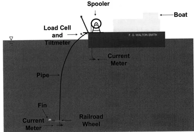
3.2.2 The Gulf Stream Experim ents... 50

3.2.3 The Second Gulf Stream Experim ents... 53

3.3 Key data analysis procedures... 55

3.3.1 Calculating Norm al Incident Current Profiles ... 55

3.3.2 W orking in the frequency Dom ain... 58

3.3.3 Establishing steady state regions... 58

4. Drag Coefficients ... 61

4.1 Spatially averaged mean drag Coefficients at High Mode Number: Lake Seneca Experim ents... 63

4.1.1 Methodology to calculate spatially averaged Mean Co using Observed Top Inclination Angle... 64

4.1.2 Results 68 4.2 Drag in traveling wave environm ents ... 70

4.2.1 Drag as a indicator of the wake... 70

4.2.2 Drag in Sheared Current Environm ents ... 71

4.3 Using Strain to calculate m ean drag force ... 72

4.3.1 Theory ... 72

4.3.2 Im plem entation ... 74

4.3.3 Error Analysis and discussion... 80

4.3.4 Example... 82

4.3.5 Proof of Concept ... 89

4.3.6 Drag Coefficients for bare pipe in Shear Currents... 93

4.4 Spatially averaged Drag coefficients ... 101

4.5 Drag Coefficients of Strakes and Fairings ... 101

4.5.1 Strakes 102 4.5.2 Drag for fairings...104

4.6 Sum m ary and Conclusions...106

5. The Higher Harm onics in VIV ... 109

5.1 M ain Conclusions ... 109

5.2 Introduction... 110

5.3 Experim ental observations of the higher harm onics... 110 10

5.3.1 Lake Seneca experiments... 112

5.3.2 The Gulf Stream experiments ... 113

5.4 Properties of the Higher Harmonics... 118

5.4.1 The spatial variation of X,Y trajectories and its influence on the Higher H arm onics ... 122

5.4.2 Properties of the Cross-Flow Harmonics... 132

5.4.3 The in-line harmonic components... 143

5.4.4 Higher harmonics magnitudes at the boundary... 148

5.5 Results and conclusions ... 149

6. Incorporating the higher harmonics in VIV fatigue estimates... 153

6.1 Higher Harmonic Contributions to fatigue in experimental data... 153

6.2 Data properties that are important for fatigue calculations... 155

6.2.1 Probability Distribution Function (PDF) from zero-mean time series 157 6.2.2 Spectral content of the data time series... 157

6.3 Properties of the Gulf Stream strain data ... 160

6.4 In-line vs Cross-flow fatigue damage ... 162

6.5 Estimating cross-flow fatigue damage due to the higher harmonics ... 163

6.5.1 Method 1 - Using a factor to incorporate the fatigue damage due to the higher harmonics... 163

6.5.2 Method 2 - Using broadband spectral techniques ... 165

6.5.3 Suggested Practice for Engineers... 173

6.6 Main Results and Conclusions... 175

7. Conclusions and Future Work ... 177

7.1 D rag due to V IV ... 177

7.2 Higher Harmonics in VIV... 177

7.3 Fatigue damage due to VIV ... 178

APPENDIX A - Details of the Mechanical Design for the Second Gulf Stream Experiment

Appendix B - Depth Sensor

Appendix C - More results on the Higher Harmonics in VIV

Appendix D - Weibull Distribution to represent the 1st harmonic stress range

LIST OF TABLES

Table 1 -Lake Seneca Pipe Properties ... 49 Table 2-Gulf Stream Pipe Properties ... 53 Table 3 - Details of the pipe used in the second Gulf Stream Experiments ... 54 Table 4 - Calculations using nominal values for the second Gulf Stream experiments show that pipe was stiffness dominated... 74 Table 5 - The ratio of the RMS 3x strain to RMS lx strain for all tests... 135 Table 6 - The ratio of RMS 3x strain and RMS lx strain for steady-state regions in the

second Gulf Stream experim ents... 135 Table 7 - The analysis of steady state cases reveals a conservative estimate of the 5th

harmonic strain response. The ratio refers to the ratio of the maximum RMS 5th

harmonic response to the maximum RMS 1st harmonic response... 138 Table 8 -The analysis of small time length steady state cases provided a mean estimate

of the maximum RMS 5th harmonic strain response. Ratio is the maximum RMS 5th

harmonic strain response divided by the maximum RMS 1st harmonic strain

response ... 139 Table 9 - The maximum 2x and 3x RMS strain response is a fraction of the maximum

observed 2x and 3x RM S response for a test... 149 Table 10 - The ratio of the maximum in-line fatigue damage (at any location on the

pipe) to the maximum cross-flow fatigue damage (at any location on the pipe).. 162 Table 11 - The contribution of the 1st harmonic fatigue damage is overestimated when

the Rayleigh formulation is used. The Rainflow method is taken as the standard for this com parison ... 164 Table 12 - The amplification in fatigue damage due to the higher harmonics for 9

different bare pipe tests from the second gulf stream experiments ... 164 Table 13 -Dirlik method predicts damage more accurately than the Rayleigh method for broadband spectra ... 169 Table 14 -Results using the "Modified Dirlik" approach compare well with the Dirlik method. A ratio of 1 in the table indicates an exact match with the fatigue damage estimated using the Rainflow counting method... 172

Table 16 - The 2x-tolx ratio for full tests provides the a mean estimate of the strain response at the 2x harmonic in terms of the measured or estimated lx response. 206 Table 17 - The 2x-tolx ratio for steady-state regions provide another estimate of the strain response at the 2x harmonic in terms of the measured or estimated lx resp on se ... 206 Table 18 - The 4x-to-lx ratio for the 4th harmonic for steady state cases shows the a high

mean value but also a large standard deviation ... 208 Table 19 -The 4x-to-lx ratio for the 4 th harmonic using unsteady cases shows a smaller

mean value but the standard deviation is still large... 208 Table 20 - Fatigue damage calculations that use the Rayleigh method to calculate stress range PDFs produce overly conservative results for the lx VIV data measured during the Gulf Stream experim ents...210 Table 21 -Weibull distribution, with k =4 and2 A =l.1mo, predicts fatigue damage better

than the Rayleigh method when compared to the Rainflow counting method. A value of 1.0 in the table would indicate an exact match with the Rainflow fatigue dam age estim ate...2 14 Table 22 - A comparison of fatigue life estimates at four sensor locations for Test

-20061023203818 from the second Gulf Stream experiments. The table indicates that the Weibull distribution predicts fatigue damage more accurately than the Rayleigh method when compared to the Rainflow counting method. (k =4 and = l.lm o)... 2 18

LIST OF FIGURES

Figure 1 - The progression of the oil and gas drilling and production operations into deeper w ater... 25 Figure 2 -VIV is a ubiquitous phenomenon that is seen over a wide range of Reynolds numbers and wide ranging physical situations... 27

Figure 3 - Free vibration experiments with a 1 degree-of-freedom rigid cylinder by

Overvik (1982) (taken from Sarapkaya, 2004)... 39 Figure 4 -Drag Coefficient contours for force experiments at Re=10,000. (From 28).... 40

Figure 5 -(a) Mean drag coefficients from 1-D free vibration, rigid cylinder experiments (from 29) and (b) Mean drag coefficients from 2-D free vibration, rigid cylinder

experim ents (from 6)... 41

Figure 6 - The figure 8s were noticed by Vandiver in the lock-in regions in a flexible pipe undergoing V IV ... 45 Figure 7 - The A/D of a spring mounted rigid cylinder in free vibration with both in-line and cross-flow degrees of freedom. For the x-axis, reduced velocity is based on the measured ,response frequency of the cylinder... 46 Figure 8 -Setup for the Lake Seneca experiments... 50

Figure 9 - Stow position and the deployed position during the second Gulf Stream

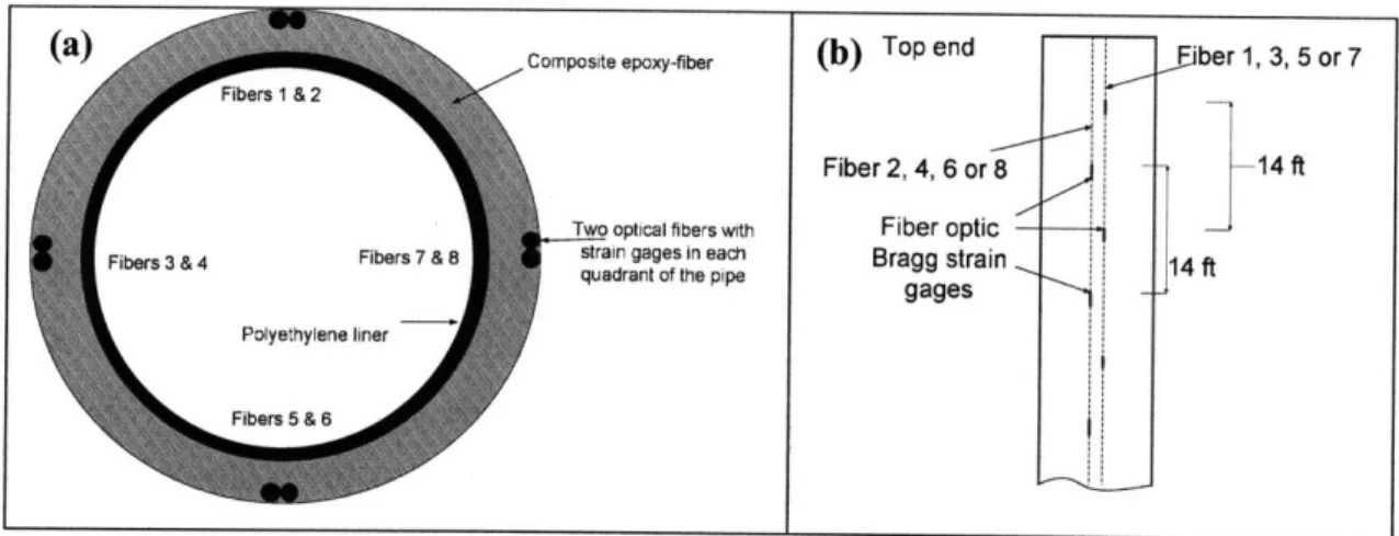
experim ent... ... 51 Figure 10 - (a) Cross-Section and (b) Side View of the Pipe from the Gulf Stream Test

... ... . . ... ... .... 52

Figure 11 - Pressure Transducer (left) installed in an aluminum casing to the rail road w h eel... 55

Figure 12 (a) -Time-Frequency plots for test 20061023203818 show that in this example

steady state conditions are achieved only in the last 60 seconds. The plots were obtained using the Morlet Wavelet analysis. (b) The normal incident current profile with locations where the wavelet transforms shown in (a) were performed... 59 Figure 13 -Strain PSDs, shown for Q4 and Q1, in the steady state region are almost single frequency responses. Each PSD was calculated using the Welch method with 60 seconds of data, a 40 second window length and 95% overlap... 60

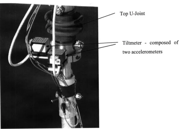
Figure 14 - Accelerometers in the Lake Seneca experiments were used to get top tilt an g les ... 6 5

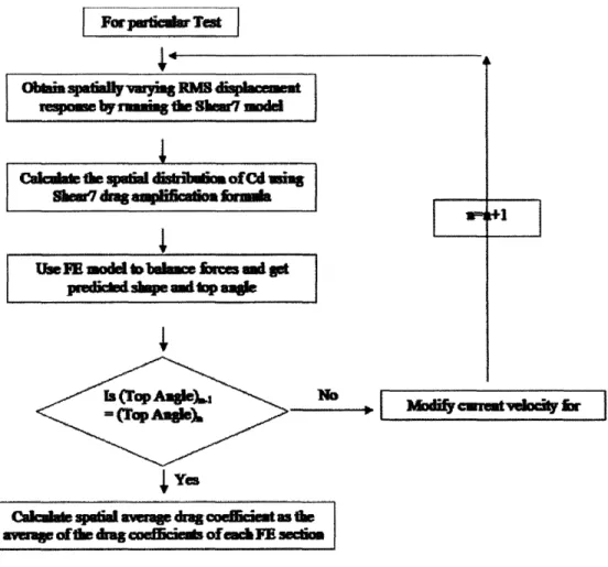
Figure 15 - Method 1: Spatially averaged mean CD values calculated using SHEAR7

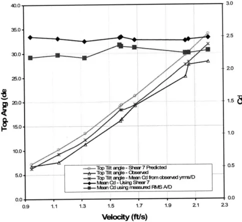
predicted displacement response. Note n indicates the iteration number... 66 Figure 16 -Method 2: Spatially averaged mean CD values are calculated using measured displacement response (calculated from acceleration data). Note n indicates the iteration num ber... 67 Figure 17 - Estimated drag coefficients (left axis) and top tilt angles (right axis) for different tow speeds using data from the Lake Seneca experiments with 401 ft long p ip e ... 6 9 Figure 18 -Drag coefficients estimated from Lake Seneca experiments -201 ft long pipe

... 7 0

Figure 19 - Schematic showing that the mean normal force can be found if the tension and curvature are know n... 73 Figure 20 - The sum of Residual Strains and axial strains due to the weight of the RRW and pipe for bare pipe tests performed on the 2 3rd of October, 2006, the 4th day of testing. Q1, Q2, Q3 and Q4 indicate the quadrants where the fibers are located.... 75 Figure 21 -The sum of residual strains and axial strains due to the weight of the RRW and pipe for quadrant 1 on three different days of testing. Their difference shows how creep changed the residual stresses during the Gulf Stream experiments ... 76 Figure 22 - The mean strains for each quadrant from the zero file 200623201203. The zero file gives the residual strains and tension strains that have to be removed from the measured mean strains for a particular experiment ... 83 Figure 23 - (a) The zero for this test has to be removed from the temporal mean of the measured experimental strain, shown in (b)... 84 Figure 24 -(a) The (measured-Zero) strain for each fiber includes the static bending strain and changes in local mean tension during tow (b) fiber pairs (Q1,Q3) and fiber pairs (Q2,Q4) are used to estimate mean tension during tow ... 85 Figure 25 - (a) The total static bending strain of the pipe and (b) the associated drag fo rce ... 8 6

Figure 26- The distribution of local drag force, shown in (a), is used in conjunction with the normal incident velocity profile, shown in (b), and the properties of the pipe to estimate the local drag coefficient along the length of the pipe ... 87 Figure 27 - The spatial distribution of local Co for Test-20061023205043. The red lines indicate CD + 1 standard deviation of the error ... 88 Figure 28 - The contribution of the three parameters to the standard deviation of CD

shows that the main cause of the large error in CD towards the top end of the pipe is the error in strain m easurem ents... 89 Figure 29 -(a) A schematic showing the 40% fairings setup. (b) A picture of the fairings during the experim ents ... 90 Figure 30 - Four different velocity profiles for the 40% fairing cases. The Fairings were attached at the end of the pipe (as shown in the figure). The profiles were chosen to cover the range of velocities tested during the experiments... 91 Figure 31 - CD variation along the length of the pipe for four Gulf Stream experiments with fairing covering the bottom 40% of the pipe... 92 Figure 32 - Local drag coefficient along the length of a bare pipe in a typical Gulf Stream case... ... 94

Figure 33 - Drag coefficient plotted against reduced velocity in (a) for Test

-20061023205043 from the Gulf Stream experiments where the reduced velocity changed due to the shear in the current (b) free vibration experiments with a 1 degree of freedom rigid cylinder by Overvik (1982) (taken from 16)... 95

Figure 34 - (a) The velocity profile and (b) the associated local drag coefficients for three bare pipe tests from the second Gulf Stream experiments. The region of pronounced drag is clearly seen in all the experiments... 97 Figure 35 - The variation of local drag coefficient (a) along the axial length of the pipe

and (b) with local reduced velocity. The results are for Test-2450 and Test-2490 from the NDP experiments. Bottom indicates the end where the velocity was high.

... 9 9

Figure 36 - Local drag coefficients with error bars (shown with red lines) (a) Test-2450 (b) Test-2490 from the NDP experiments. Bottom indicates the end where the velocity w as high ... 100

Figure 37-Spatially averaged drag coefficients for bare pipe tests performed during the Gulf Stream experiments have values similar to those observed in the Lake Seneca exp erim ents... 10 1

Figure 38 - The drag coefficients for strakes used in the Lake Seneca experiments, 0.25 D height and 17.5 D pitch, were found to be between 1.1 and 1.5... 102 Figure 39- Two different stake coverages were tested during the second Gulf Stream exp erim ents... 103 Figure 40 - The mean drag coefficients for the different strake coverage amounts for different top angles. Higher top angles indicate a higher tow velocity ... 104 Figure 41 - Two different amounts of fairing coverage were tested during the second G ulf Stream experim ents... 105 Figure 42 - The mean drag coefficients for the different fairing coverage amounts for different top angles. Higher top angles indicate a higher tow velocity ... 106 Figure 43 - The amplitude of the 3rd harmonic, when compared to the amplitude of the

1st harmonic, is nine times greater in acceleration or strain data than in displacem ent data... 111

Figure 44 - Cross-flow and in-line acceleration PSDs showing the energy at the 1st and the higher harmonics observed in the lake Seneca experiments. The harmonics are indicated as lx, 2x etc. (a) z/L = 0.19 from the top end and (b) z/L = 0.77 from top end. The units for both (a) and (b) are (m/s2₎2_{/Hz ... 113}

Figure 45 - (a) - Time-Frequency plots for test 20061023203818 show steady state

conditions are achieved only in the last 60 seconds. (b) The normal incident current profile with locations of the time-frequency analysis shown in (a)... 114 Figure 46 - Strain PSDs for Quadrants 1 and 4 at 3 different axial locations show the

higher harmonics in the VIV response. Test - 200623203818 ... 115 Figure 47 - The total cross-flow strain spectrum (odd harmonics) and the total in-line

strain spectrum (even harmonics) at 3 different locations on the pipeTest

-200623203818 ... 117

Figure 48 - The axial distribution of total cross-flow RMS strain and the RMS strain from only the 1st harmonic for Test-200623203818... 117

Figure 49 - The phase relationship between the in-line and cross-flow motion leads to different displacem ent patterns... 123 Figure 50 - (a) The RMS strain response at the lx, 2x and 3x frequencies during a 3

second time period (b) The magnitude of the 1st harmonic clearly shows regions of standing and traveling waves (red=peak, blue--trough)... 124 Figure 51 - The region of enhanced local drag coefficient (shown in (a)) is also the

region where the traveling wave is starts propagating along the pipe (shown in (b)).

... 12 5

Figure 52 - X,Y plots in the standing wave region. Current direction is from bottom to top ... 12 9

Figure 53 - The X,Y trajectories in the traveling wave region of the pipe where the phase difference between the lx and 2x motion is 180 degrees. Current direction is from bottom to top... 130 Figure 54 - The X,Y trajectories show a 'figure c+8' pattern (Sensors 34,35) which corresponds to a 45 degree phase difference and a large 3x response. The phase changes to 90 degrees leading to a 'figure c' pattern (sensor 32,33) and large 2x response. Finally the trajectory direction is reversed as the phase crosses 90 degrees (sensor 30,31). Current direction is from bottom to top... 131

Figure 55 -RMS 1st and ₃rd harmonic strain for test 20031023205557 ... 132

Figure 56 - The reduced velocity of the maximum RMS strain in the lx and 3x

frequencies are very close to each other ... 133

Figure 57 - The cross-flow components 3x and lx RMS strain show no trends. The 3x

RMS and 2x strain, which are in the cross-flow and in-line direction, show a clear dependence on one another. The data is from experiments on the 20 th, 2 1st and 2 3rd of O ctober, 2006 ... 136

Figure 58 - Comparison of the reduced velocity of the maximum 3rd harmonic response

and the maximum 5th harmonic response ... 138

Figure 59 - The maximum normalized RMS 5x strain shows a clear trend when plotted

against the maximum normalized RMS 4x strain. The data is from experiments on the 20t , 21st and 23rd of October, 2006 ... 141

Figure 60 - The normalized RMS 5x strain shows clear trends when plotted against the shear param eter... 142 Figure 61 -RMS 1st and 2nd harmonic strain for test 20031023205557 ... 144

Figure 62 - The region of maximum response of the lx and 2x RMS strain for Test

20061023205557 is plotted against (a) axial position of the pipe where 0 is the bottom end and (b) reduced velocity ... 144

Figure 63 - The reduced velocity at which the maximum lx RMS strain is always higher

than the reduced velocity at which the maximum RMS 2x strain occurs. Results from 11 different tests are shown here ... 145 Figure 64 - A strong correlation is observed between the peak 1st harmonic response

and the peak 2nd harmonic response. The data is from experiments on the 20th,

2 1st and 23rd of O ctober, 2006 ... 146 Figure 65 - The reduced velocity at which the peak RMS 4th harmonic strain is observed

is close to the reduced velocity at which the peak RMS 1st harmonic strain is ob served ... 147

Figure 66 - Maximum normalized 4x and 2x RMS strains show no dependence on each

other. The data is from experiments on the 20th,

2 1st and 2 3rd of October, 2006.. 148 Figure 67- Comparison of fatigue damage predicted by Shear7V4.5 to that calculated from measured data using the Dirlik method. Young's modulus for steel and API-X ' S-N curve w ere used...154

Figure 68 - The ratio of the total cross-flow damage to the maximum damage by

SHEAR7-V4.5. The ratio at sensors 33, 43 and 53 are shown by solid dots... 156 Figure 69 - The ratio of the total damage rate to the maximum lx damage rate in the

same region, which occurs at z/L=0.2. The ratio at sensors 33, 43 and 53 are shown by solid dots... 156 Figure 70 -Distribution of time series data generated from Shear7 output ... 158 Figure 71 -(a) An example of a broadband spectrum (b) and example of a narrow band

sp ectrum ... 158 Figure 72 -Amplitude variation with time for a narrow banded spectrum... 159 Figure 73 - Measured Strain compared to the lx component for an example case from the first Gulf Stream experim ents... 161

Figure 74 - The probability distribution of normalized strain amplitude (normalized using its variance) at four sensor locations. The data was first filtered to remove the higher harm onics ... 161

Figure 75 - A model for the strain response at the 3rd and 5th harmonic frequencies based

on observed properties from the second Gulf Stream experiments... 166 Figure 76 - The distribution of the Gulf Stream Q2 Strain data at a representative location (sensor 53 - 372.5 ft. from the top) in (a) the frequency domain using a PSD (b) time domain using the probability distribution of strain amplitude

normalized by the variance of the data. Also shown in (b) is a Gaussian probability

distribution (m ean=0, variance=l) ...

167

Figure 77 - The most widely used formulation to get stress range PDFs from broadband

spectra is by Dirlik and uses the zeroth, 2nd and 4th spectral moments in its

form ulation ... 168

Figure 78 - Strain PSDs and corresponding stress range PDFs at 3 sensor locations (sensor 33 - 232.5 ft., sensor 53 - 372.5 ft., sensor 57 - 400.5 ft.)... 169 Figure 79 -Strain PSDs and corresponding stress range PDFs at 3 sensor locations... 171 Figure 80 - Total cross-flow strain predicted using the proposed method matches well

with the measured total cross-flow strain. The x-axis shows RMS strain... 174

Figure 81 - The distribution of fatigue damage using SHEAR7 with the proposed

method compares well with results from actual measured strain data, especially in the region of m aximum dam age ... 174 Figure 82 -3D model of the spooler and base structure 187

Figure 83 -The top end connection when (a) deployed (b) stowed on the drum... 189 Figure 84 -Sketch of the top end connection ... 190

Figure 85 -(a) Details of the cradle and bolt mechanism to keep the bar secure during the tests (b) Details of the collar-bar setup during operation... 191

Figure 86 - (a) RailRoad Wheel with the spindle in position (b) The bottom end

connection during the experim ents... 192

Figure 87 -Bottom connection details... 194 Figure 88 - Aluminum casing for pressure transducer... 196

Figure 89 - (left) Pressure transducer (right) direction vane and pressure transducer installed on the Rail Road W heel fin angle ... 197 Figure 90 - Calibration Curve for Direction Vane... 198 Figure 91 - Bottom End Connections ... ... 199 Figure 92 - (a) lx RMS micro strains from two orthogonal quadrants (Qi1 and Q4) and (b) 3x RMS micro strains from the same two orthogonal quadrants... 201 Figure 93 - When the 3rd harmonic strain time series is plotted agaist the 1st harmonic

strain time series in steady-state regions, the shapes remains constant in time indicating that the 3rd harmonic is phase locked to the 1st _{harmonic... 202}

Figure 94 - The X,Y trajectories when the region of maximum 3x RMS response shows

a phase difference of around 180 degrees between the inline and cross-flow motion.

... 2 0 3

Figure 95 - The X,Y trajectories in the region of maximum 2x response for (a) Bare Pipe test 20061023203818 and(b) Bare pipe test 200610233200. The plots show a 'figure c' pattern ... ... ... ... 207 Figure 96 - Maximum normalized 4x RMS strain shows good correlation with the shear p aram eter ... 2 0 9 Figure 97 - Comparison of Rainflow cycle counting and Rayleigh PDF's for stress range distributions ... . ... ... ... 211 Figure 98 -Variation of Fatigue damage with k for different values of A ... 213 Figure 99 - A comparison of the stress range PDFs shows that the Weibull distribution

with k=4 and A=1.1 mo is a better approximation of the stress range PDF obtained from Rainflow counting methods. ... ... 214

Figure 100 -The RMS micro strain from Test- 20061023203818 for Q2 and Q1 shows

the region of maximum strain around the center of the pipe. (b) The mean normal current profile for the experiment with the green dots showing the four locations that w ere studied in detail... ... 215 Figure 101 - (a) Spectra at four different locations from Test - 20061023203818 shows

the presence of the higher harmonics. (b) Filtered spectra that were used to check the accuracy of the proposed Weibull stress range PDFs... 216

Figure 102 - The stress range PDFs from the proposed Weibull distribution matches those obtained from Rainflow counting methods. The four locations correspond to sensors 40 (-281.6 ft), 46 (-323.6 ft), 52 (-365.6 ft) and 58 (-407.6 ft) ... 217

1. Introduction and Motivation

1.1 Introduction

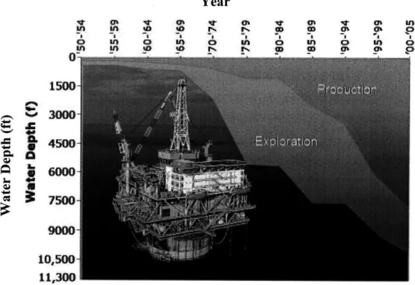
Most unexplored oil and gas reserves of significance are offshore, miles away from any coastline. Having exhausted much of the onshore and near-shore reserves, the oil and gas industry is moving into deeper waters to find large reserves to meet the growing energy demands. Figure 1 shows the timeline of the oil and gas industries progression into deeper waters. They are also drilling in harsher environments for oil and gas. In their quest, one of the many challenges they face is that of Flow-Induced Vibrations (VIV).

Year

1500

o000

11,300

Figure 1 - The progression of the oil and gas drilling and production operations into deeper water

For many years, amplification in drag and fatigue damage due to vortex-induced-vibrations (VIV) has caused significant problems for offshore platforms and risers operating in strong ocean current environments. The problem has been aggravated in recent years as water depths increase and the risers are excited at higher modes. In just

VI

am

the last few years there have been several high profile rig failures because of reasons that can, at least partially, be attributed to Flow-Induced vibration 1.

Expectedly, extensive VIV research has been carried out over the last fifteen years. This has led to significant understanding of the physics behind VIV and the occurrence and behavior of these vibrations in constant and sheared current profiles. This understanding has resulted in the development of VIV prediction programs like SHEAR7' that estimate the effects of VIV on slender structures.

Despite these advances, VIV is still not clearly understood and many important questions regarding it, especially in sheared current profiles, remain unanswered. As a result, the oil and gas industry uses design safety factor of ten or higher for VIV related

fatigue damage in spite of predictive programs generally giving conservative estimates of displacement response due to VIV.

1.2 Background

It has long been observed that flow of a viscous fluid past a bluff body creates vortices in its wake, which are shed alternately from both sides in a pattern called the Karman Vortex Street. This phenomenon is quiet ubiquitous, see Figure 2, and can be seen when air flows past thin strings, like the Aeolian harp, or in the clouds when their flow is interrupted by a mountain or island. These alternating vortices create a periodic forcing on the bluff body which becomes important only when their shedding frequency is close to one of the natural frequencies of the bluff body. Then the bluff body shows resonant behavior and vibrates with large amplitudes. The resulting vibrations are known as Vortex Induced Vibrations or Flow-Induced Vibrations.

SHEAR7 is a VIV prediction program owned and maintained by Dr. J. Kim Vandiver at MIT. For details visit httD://web.mit.edu/SHEAR7/SHEAR7.html

Re-10-2 - An image from a Scanning Electron Microscope (SEM) showing the formation of the Von Karman Vortex street behind a Tin particle in flow of Argon gas. The application in this case is growing Silicon nanowires 2

Re-102

- _{The Saint Louis wind harp is 13 feet high in}

Blind Boone park located 60 miles east of Kansas City, MO.

Re-104

- A typical vortex shedding pattern seen behind a cylinder placed in fluid flow. Experiments at these Reynolds numbers are common with VIV researchers.

Re-~107 - Spar platforms, used in the oil and gas

industry due to their low heave response to ocean waves, are prone to Vortex-Induced Motion (VIM).

Re-10" - _{Von Karman Vortex streets seen behind}

small islands in the Alutian Islands in the northern Pacific ocean. The image, acquired by Landsat 7's Enhanced Thematic Mapper plus (ETM+) sensor, shows the wake behind the islands when fast moving clouds encounter them.

Figure 2 - _{VIV is a ubiquitous phenomenon that is seen over a wide range of}

Reynolds numbers and wide ranging physical situations. 27

1.2.1 Brief History of VIV

Centuries ago, Leanardo Da Vinci painted the Karman vortex street he observed behind some pilings in a stream. Later, Strouhal, in 1878 measured the acoustical notes from vertical wires revolving about a parallel axis and expressed the frequency as f = (0.185 x U)/D, where U is the speed of air flow onto the wire and D is the diameter of the wires. This suggested that the non-dimensional number (f x D)/U is a constant and is called the Strouhal number. This formula has been subsequently modified by Lord Rayleigh in 1915 (see 3) and again by Roshko in 1954 (4) to account for slight variations in the Strouhal number with viscosity but it remains remarkably constant for a wide range of Reynolds number and shapes of bluff bodies. The vortex shedding frequency, fs, is expressed as fs = (St x U)/D, where U is the fluid flow speed, D is the diameter of the bluff body and St denotes the Strouhal number with a value of around 0.2. During "lock-in", the response frequency of the body is very close to the predicted vortex shedding frequency.

Von Karman's theoretical work in early 20th century, which explained the stable alternating vortex shedding pattern behind bluff bodies, laid the theoretical groundwork for VIV research. However, it was not until the 1960s and 1970s that extensive work was undertaken to explain VIV and incorporate its effects into engineering design. Results from field experimental in the 1980s, by Vandiver et al. 5 and others, provided greater understanding about the drag and lift aspects of VIV, and paved the way for empirical programs for the prediction of VIV.

The 1990s and the first half of this decade has been filled with carefully done research in laboratory environments, which have shed light on the subtleties of VIV. For example, in 2003, Jauvtis and Williamson 6 showed that VIV amplitude response of a rigid cylinder was larger when both in-line and cross-flow motion were allowed as opposed to just cross-flow motion. Similarly, Triantafyllou et al. in 2004 examined the amplitude response in the in-line and cross-flow direction for rigid and flexible cylinders in constant currents and found that in flexible cylinders, unlike rigid cylinders, the peak

displacement response in the in-line direction did not occur at the same reduced velocity and the peak displacement response in the cross-flow direction.

The study of long flexible cylinders, the kinds used in the oil and gas industry, has just begun. Only recently have Vandiver et al. 8"10performed a series of experiments that approximate the large length-to-diameter ratios seen in real oil and gas structures, albeit at lower Reynolds numbers. These experiments have were key in identifying important areas of research like the higher harmonics, their affect on strain and traveling waves response of long flexible cylinders responding at high modes to highly sheared current profiles. Just when the VIV research community was beginning to believe that they understood the complex nuances of VIV, these experiments provided a stark reminder that much work still needs to be done.

1.2.2 Complicating Issues

A sense of the complicated nature of VIV can be obtained from the general equation of motion for any point on a pipe undergoing VIV, shown in Equation(1.1). In most cases, Equation(1.1) is simplified by decoupling the x and y motion. Even then, the dependence of added mass and damping on displacement, axial position, and frequency makes it difficult to solve the equations without making simplifications. The dependence of the forcing on the displacement adds further complications to the problem requiring an iterative process to solve the equation 11. Further difficulties are posed by the three dimensionality of the problem. The forcing due to a three dimensional wake can be significantly different from the two dimensional wake which is assumed to simplify the problem.

(m(z) + m. (x, y, z, wo))y,, + c(x, y, z, co)y, + (EI(z)y. - T(z)y.) = F(x, y, z, t)

where

m(z) = local mass density m (x, y,z, o) = local added mass

c(x, y, z, co) = local damping (1.1

EI (z) = local bending stiffness T(z) = local Tension

Secondly, the structures in the oil and gas industry to which the VIV problem most applies further complicate the problem. Deepwater risers can have length-to-diameter (L/D) ratios greater than 5000, Spar and deepwater semi-submersible platforms operate in the Reynolds number regime of 107 or greater. These massive sizes, and the non-dimensional parameters associated with it, make it difficult to build and test models that effectively represent the actual structure.

Thirdly, the hydrodynamics of the vortices are difficult to theoretically predict and visualize. The vortex shedding patterns change with various non dimensional parameters like reduced velocity and Reynolds number. Figure 3 shows the various vortex shedding

patterns from laboratory experiments done by Williamson and Roshko 12 in which the

in-line motion was restricted. Each of these patterns produces a different hydrodynamic force, lift and drag, on the structure. Moreover, the vortex shedding patterns are different if in-line motion is not restricted for the structure.

0.

X/D

0 0-2 0-4 0.6 08- 1-0 162 1-4 [-6 1-8 2.0

A-,/ 7, Figure 3 - Map of vortex synchronization

region; from Williamson and Roshko [10].

30

Visualizing the vortex pattern in the wake of a cylinder is a difficult, expensive and time consuming task. Some of the experimental techniques are Digital Particle Image Velocimetry (DPIV), pressure-sensitive color dyes and time resolved PIV. Recent progress in Computational Fluid Dynamics (CFD) has also made it possible to visualize the formation and propagation of these vortices as shown in Figure 3. They too, however, come with a staggering cost in terms of computation time, modeling and coding effort, and computing power. Furthermore, in spite of the phenomenal increase in computation speeds in recent years, CFD methods still have difficulty solving the Navier-Stokes equation at Reynolds numbers encountered in the offshore oil and gas industry. This motivates research in finding other ways that provide information about the wake without the time and cost penalty associated with the techniques mentioned above.

Figure 4 - Recent advances in CFD programs has led to accurate predictions of the vortex dynamics in the near wake of a cylinder undergoing VIV

Finally, the current profiles that are seen by the real structures pose additional problems. Most laboratory experiments, motivated by simplicity in the experimental setup and analysis, introduce a constant velocity fluid flow on a spring mounted rigid cylinder. The reduced velocity is varied by changing the current velocity. In realistic current flows, shear in the current can cause the local reduced velocity to vary along the riser. Further, VIV data from laboratory experiments is dominated by rigid cylinder motion or standing waves in flexible pipes. However, in deepwater risers in sheared currents, the response is mostly traveling waves. This discrepancy in the experimental data and the reality has not been studied in detail.

1.2.3 Things that matter most to the oil and gas industry

While it is important to recognize the complexity of the VIV problem, it is imperative to remember the physical quantities that are most useful in design of offshore structures. It may be that the quantities of interest can be approximately predicted without incorporating all the details of the physics of the VIV problem. The quantities that are of most interest to the offshore oil and gas industry are displacement response of a structure due to VIV, drag force amplification due to VIV and the fatigue damage caused to VIV.

1.2.3.1 Displacement response of a structure due to VIV

The offshore industry uses a lot of cylindrical structures in their operations that are prone to VIV. Moreover, many of these structures are close to other structures and their displacements due to VIV or VIM have to be predicted accurately, making the VIV displacement response prediction a key area of research.

Recent work indicates that VIV predictive programs do a good job in predicting the cross-flow displacement response due to VIV 1o. The prediction process is hampered by the difficulties discussed earlier, but programs like SHEAR7 are able to estimate the region and magnitude of the maximum response fairly accurately.

A critical step in the VIV prediction process is estimating correctly the "power-in" region, where the structure takes energy from the fluid. Though laboratory experiments have developed guidelines where "power-in" regions should occur, more research is underway to identify the position and length of these regions on structures placed in realistic ocean currents. Further, identifying and defining these regions becomes harder when traveling waves are present. The current thought is that a standing wave forms in the "power-in" region and energy is dissipated as traveling waves from the ends of the "power-in" region. This theory is being questioned based on data from the Gulf Stream

experiments. Figure 5 uses test data from the second Gulf Stream experiments and

shows regions of traveling wave and standing wave VIV response. More research is required to identify the "power-in" regions in the traveling wave environments.

d 3C

z

A

6CO

tim(s)

Figure 5 - A plot of amplitude of VIV with time for each sensor clearly reveals the existence of traveling waves. Following peaks, shown in red, and troughs, shown in blue, in time indicate regions of standing and traveling waves. The example was from the Test - 20061023203818 from the second Gulf Stream experiments.

1.2.3.2 Drag forces amplification due to VIV

Accurate force estimates are required for any structural design and the marine risers and offshore structures are no different. Drag forces are estimated by semi-empirical formulations used in VIV prediction programs like SHEAR7. These formulations were developed many decades ago based on field and laboratory experiments. However, many aspects of VIV, especially traveling wave response, were not fully understood then. The formulations therefore were developed based on data that did not represent the response of an offshore structure. These drag force formulations were obtained by using force

measurements at the ends of the flexible cylinder and thus producing spatially averaged forces. However, estimating drag forces when the local reduced velocity changes and the response is mostly in the form of traveling waves has not been researched primarily because it has not been possible to measure the local drag coefficients in long pipes where the local reduced velocity changes due to shear in the current.

1.2.3.3 Fatigue damage due to VIV

The offshore oil and gas industry uses the SN curve method of fatigue damage estimation fatigue damage, which is arguably the most important consequence of VIV. The thinking for a long time has been that if the displacement response due to VIV is predicted correctly, then the stress response computed from this displacement response can be calculated easily making the assumption that the response is at the fundamental frequency of VIV, which corresponds to the Strouhal frequency. However, recent experiments 8, 10 have indicated that stress spectra obtained from VIV strain measurements contain energy at frequencies that are multiples of the Strouhal frequency. Moreover, the strain at these higher frequencies is caused due to the high curvature associated with these high modes and not due to high displacement amplitude of vibration. This means that these higher harmonics could contribute greatly to the fatigue damage due to VIV without significantly affecting the displacement response due to VIV. This provides the motivation to understand these higher harmonics so that they can be predicted and their effects incorporated into fatigue damage estimates used in the

industry.

Even before the effects of the higher harmonics are incorporated, the current estimation fatigue damage calculation process has to be reevaluated. Various assumptions, like VIV strain being a Gaussian process, have never been carefully verified. However, these assumptions are used as justification for the use of the Rayleigh formulation 13 in the fatigue estimation process.

1.3 Motivation for this Work

The above descriptions of the problems we face in solving VIV problems coupled with the quantities the oil and gas industry is most interested in provides some very

interesting areas for research that will have the maximum impact on VIV related engineering design procedures in use today. The first of these is the need to be able to predict the "power-in" regions in traveling wave environments. The scarcity of well instrumented data sets showing traveling waves makes it difficult to move forward on this front. However, innovative methods that can indirectly point out the "power-in" regions can be very helpful moving forward. This is particularly true because the currently accepted theory of the "power-in" having standing waves does not seem to work when most of the vibrations are in the form of traveling waves.

The second area that clearly needs more insight is the variation of drag coefficients in traveling wave environments. A plethora of drag-related data is available on rigid cylinder experiments where the variation of drag coefficients has been established with reduced velocity. However, little is known about the variation of reduced velocity in sheared current environments where the reduced velocity changes with the spatial location on a pipe. Further, the drag coefficient formulations in use today were developed using data from rigid cylinder laboratory experiments or field experiments that had standing wave VIV response. They, however, are used in sheared current environments for existing projects where the response is dominated by traveling waves. No research has been carried out verifying their accuracy in such environments. Further, no established methods exist to compute drag coefficients using data from highly instrumented pipes undergoing VIV.

Such a method offers promise to address the concerns of finding the "power-in" region as well. Laboratory research has shown relations between high drag coefficients and wake patterns. A similar correlation may exist between wake patterns and displacement amplitudes, phase difference between in-line and cross-flow motion and lift coefficients. Using time-averaged mean drag, or local drag coefficients, as a method to identify the wake patterns in sheared flows with traveling wave VIV response has never been proposed.

Finally, fatigue damage remains one of the most important yet least understood aspects of VIV. Recent research indicates the existence of higher harmonics in strain data measurements from VIV field experiments. When do these higher harmonics occur? What is the fatigue implication of these higher harmonics? Are the current fatigue

formulations used in the oil and gas industry adequate or will there be a need to modify them based on these new findings? The answers to these questions could have a

significant impact current design procedures in use today.

1.4 A preview of the chapters that follow

This thesis is organized in seven chapters. So far, a brief history of VIV, the important VIV related parameters that most impact the oil and gas industry and the motivation for this work, which follows from the earlier discussions, have been presented. The contents of the chapters that follow are summarized below.

Chapter 2 contains the summary of previous research that is related to this work. Due to the plethora of research done on VIV, this literature survey has been limited to the topics that pertain to the work presented in this thesis, which are higher harmonics, drag amplification due to VIV and the fatigue implications of VIV.

Chapter 3 explains the details of the experiments that provided most of the data analyzed for this research. The details of these experiments have been previously published in various reports, which is why this chapter gives a broad overview and presents details of only the aspects of the experiments that had significant contributions from the author.

Chapter 4 deals with drag amplification due to VIV. It presents a new way of calculating local mean drag coefficients, and then suggests how this could be used to infer information like the "power-in" region in pipes and the local wake structure behind the pipe.

Chapter 5 explains the observation of and research on the higher harmonics of VIV. The chapter represents the findings of the author about when the higher harmonics exist, their magnitude and properties that are used in Chapter 6 to build a preliminary model for the higher harmonics.

Chapter 6 goes into the details of fatigue damage due to VIV. This chapter examines the fatigue damage due to the higher harmonics and presents two methods of incorporating them in VIV predictions..

Chapter 7 is a summary of the main results presented in this thesis. It also contains some suggestions for future work.

2. Literature Survey

Research on VIV dates back four decades and volumes of research exist on the subject. A good understanding of the subject can be developed by reading the various books that have been written on the subject 11, 14, 15, or studying the many reviews that have been published in various journals 16-18. Therefore, the purpose of this chapter is not give the reader a review of all the significant research done in the field of VIV but only to limit the review to the topics most relevant to this thesis. Even in that, the approach is to give the reader an understanding of the history and significant work that led to the current state-of-the-art and which forms the foundation that this work builds upon. For example, the field of fatigue damage estimation has two distinct schools of thought; the people who favor the S-N curve and Miner's rule approach and those that swear by the crack propagation and fracture mechanics methods. As the oil and gas industry, and the work in this thesis, primarily uses the S-N curve approach, the fatigue aspect of the literature survey only summarizes the main contributions that led to the current state-of-the-art in the S-N curve approach.

2.1 Drag

Early research on the amplification of drag forces due to VIV was done by Bishop and Hassan 19. In forced cylinder experiments, which allowed only cross-flow motion of

the 1 inch diameter test cylinder, they measured the mean drag forces while varying the frequency of oscillation so that the ratio of the forcing frequency to the Strouhal frequency changed from below 1.0 to more than 1.0. The mean drag force peaked at a certain frequency and then decreased. They however, did not report their findings in terms of, now commonly used, dimensionless parameters like drag coefficients or reduced velocity. Moreover, the 9 inch wide and 11.25 inch deep water channel used for the experiments made it necessary for corrections due to end and blockage effects.

Griffin and Ramberg20_{, among others, studied the drag amplification of a cylinder}

oscillating in the cross-flow direction. They used a theoretical formulation of drag force based on work by Milne Thompson2 1 _{and Kochin et. al.}22 _{which required vortex strength} and spacing as inputs. They computed these inputs for experiments at Re=144 and

Re=400 and reported drag amplifications compared to stationary cylinders of around 2. Using their own and other data available at the time, they gave the empirical formula shown in Equation(2.1) for the drag amplification due to VIV. Griffin and Ramberg also correlated the length of the vortex formation region with the drag coefficients, showing that changes in the wake structure were closely mirrored by changes in the mean drag coefficients. Similar, amplifications were reported in forced vibration tests by Sarpkaya

23 and Schragel ₂₄

CD/Coo = 0.124+0.933 wr

where wr = wake response parameter

w, =(1+2 D) (St.VYT_)-' (2.1)

St= Strouhal No. (-0.2)

V

V - ; )V = Flow Velocity; f=response frequency;D=Pipe Diameter fxD

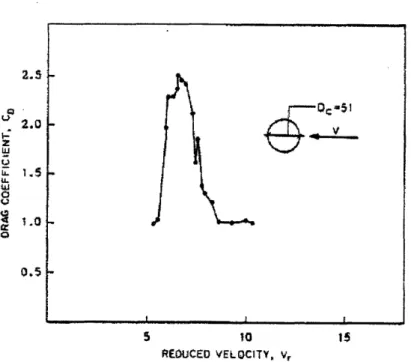
In the early 1980s, the first drag amplification values became available from spring-mounted cylinders undergoing free vibrations in uniform fluid flow. Overvik 25 plotted

the drag coefficient of a freely oscillating cylinder against reduced velocity, where the motion was allowed only in the cross-flow direction. The plot, shown below in Figure 3,

2.5 LQ 2.0 2 LU , 1.5 0 0.5 0.5 5 to 15 REDUCED VELOCITY, Vr

Figure 3 -Free vibration experiments with a 1 degree-of-freedom rigid cylinder by Overvik (1982) (taken from Sarapkaya, 2004)

Field experiments performed in the early 1980s with flexible pipes gave further credibility to the drag amplification values. In the early 1980's, Vandiver et al. conducted the first field experiments to confirm these reported drag amplifications, only observed in laboratory settings till then, for long flexible pipes in realistic current environments. Their experiments were done on a steel pipe, 75 feet in length with typical VIV excitations around modes 3 to 5. These experiments conducted by Vandiver et al. were characterized by standing waves being generated in the pipe due to the "lock-in" region covering almost the entire length of the pipe. This enabled the authors to get meaningful results from spatially averaged values of drag coefficients. Using their measurements, Vandiver et. al were able to correlate the amplitude to diameter ratio (A/D) with the amplification of drag (Equation (2.2)). It states that the predicted local CD(z) is the product of the stationary cylinder drag coefficient, CDo , for the cylinder at the operating Reynolds number and an amplification factor which is dependent on the local RMS vibration amplitude, Yr,,(z). The character "z" is the axial position coordinate along the length of the cylinder. As mentioned earlier, in the original

formulation 26 the Y,.rms(Z) term was taken to be the maximum anti-node response

S-51

VV

_

amplitude. This has proven to be too conservative, and therefore the current use of the formula 27 is to take Yrms(Z) as the local response amplitude.

CD()=

CDamp(Z) = 1.0 + 1.043 * (2 Yrms(Z))0.65 (2.2) D

In the early 1990s, Gopalkrishnan 28 did a series of experiments forced experiments

with a 2.54 cm diameter pipe. The experiments, which had Reynolds numbers of 10,000,

forced the cylinder in sinusoidal cross-flow motion. The amplitude and frequency of the motion were varied to develop a matrix of experiments. In each case, mean drag coefficients were calculated and presented in the contour plot shown in Figure 1. Though the results were similar to past work, this was the first time such a rich drag coefficient dataset was generated. It showed regions, at high reduced velocities and amplitude-to-diameter ratios in which the drag coefficient could be larger than 3.0.

1.4 1.2 1

I

I0.6

Figure 4 -Drag Coefficient contours for force experiments at Re=10,000. (From 28)

40

0o.2

n

0 0.05 0.4

···-··-···I"""··~--- I~-~ I- ~-I--^--- -I---I~

---- -- r _._...~~~~~... ·_··-

-rr-r.···-.S*a*·.lll.l.lt~l·~E.II/

.- ....

r

Though Gopalkrishnan's work was the most comprehensive drag coefficient dataset available at the time, it acknowledged the need for mean drag coefficient data from experiments that allowed both in-line and cross-flow motion in the future. This research was further explored by Charles Williamson in free vibration experiments, first with cross-flow motion only (29, 30) and then with both cross-flow and in-line motion 6.

Though he found dramatic differences in other VIV related parameters, his mean drag coefficient values, both from cross-flow motion only and in-line and cross-flow motion experiments were similar to the values observed in the forced oscillation experiments

performed by Gopalkrishnan. Figure 5 shows the plots from the Williamson paper.

CZ

2 4 a S 10 12

0 2 -4 6 8 10 12 14

Figure 5 - (a) Mean drag coefficients from 1-D free vibration, rigid cylinder experiments (from 29) and (b) Mean drag coefficients from 2-D free vibration, rigid cylinder experiments (from 6).

2.2

Fatigue Damage

Due to the implications of fatigue damage in a wide variety of subjects, it has been studied extensively over the last 150 years. Therefore, the purpose here is not to present

4 ... ... ... .... .... ... -(b) 0 ciw *! CX._{• .} # geee *.tl'• .. , o II i. , • i ; j. t •. i .• + C Q c i , . i , ~

...

..

...

A

. ..

...

..

..

...

all the work that has been done on fatigue but to highlight some of the key developments

31, 32that have led to how VIV fatigue damage is calculated in the offshore oil and gas

industry today.

According to Walter Schultz in "The History of Fatigue" 32, the first published work

on fatigue was by Wilhelm August, a German mining engineer, who in 1937 carried repeated tests on chains and winches. Schultz also mentions that the Englishman Braithwaite was the first to use the word "fatigue" in a publication in 1854 where he discussed many fatigue related failures like water pumps, railway axles and propeller shafts.

Other early work includes the study of axle failures in German railway cars by W6hler 32, 33, who was the first to suggest that different safety factors were needed for

fatigue related design and strength related design. At that time, railway accidents due to failed railway axles were commonplace. W6hler, measured the stress these axles saw during service and put forward some key observations about fatigue life like the importance of stress amplitude and mean load. He was also the first to put forward the concept of fatigue life based design, as opposed to design for infinite fatigue life, and developed tables of stress amplitude vs number of cycles to failure. These tables were the beginnings of the S-N curves that are used extensively in fatigue design. These concepts are central to the methodology used for fatigue related designs used by the oil and gas industry today.

G. Kirsh, in 1898, calculated the stress concentration around a circular hole in a large plate in tension. His finding, that stress around the hole could be as high as 3 times the value at other regions of the plate, led others like Russian mathematician Gury Vasilyevich Kolosov (1907) and British engineer Charles Edward Inglis (1914) to calculate the stress concentrations for elliptical holes. This helped engineers realize the importance of sharp corners and notches in engineering design.

In 1924, the Swedish researcher A. Palmgren introduced the concept of fatigue damage accumulation. In 1945, M.A. Miner wrote a paper "Accumulative damage in Fatigue" 34 where he also presented essentially the same hypothesis for fatigue life

summation. He also performed the first fatigue experiments to check his hypothesis. The Miner-Palmgren rule of fatigue accumulation, which states that the fatigue damage at