ECCO LLC270 Ocean-Ice State Estimate

ECCO LLC270 Ocean-Ice State Estimate

Jet Propulsion Laboratory, California Institute of Technology 12/12/2018

Summary

This document provides a brief introduction to ECCO LLC270, an ongoing global ocean-ice state estimate in the framework described by Forget et al. (2015). The estimation results are available at ftp://ecco.jpl.nasa.gov/Version5/Alpha/.

The consortium for Estimating the Circulation and climate of the Ocean (ECCO) was established to synthesize the diverse hydrographic data by the World Ocean Circulation Experiment (WOCE) and satellite sea surface height measurements by Topex/Poseidon in the early 1990s. Over the last two decades, ECCO has made significant improvements (see a recent review for OceanObs’19 community whitepaper contributed by the ECCO consortium, 2018). The ECCO framework has evolved to ECCO Version 4 (V4, see Forget et al. 2015). Now ECCO enables production of global ocean and sea-ice estimates by incorporating nearly all

observational data stream, such as measurements from Argo floats, satellite observation of ocean bottom pressure, and so on. A lower resolution ECCO state estimate (at nominal 1-degree), so-called ECCO-V4R3, covering the period 1992-2015, represents ECCO’s latest product

(Fukumori et al 2017). The production of the next-generation ECCO is aiming at higher spatial resolution (at nominal 1/3-degree). This ongoing eddy-permitting ECCO production, so-called ECCO LLC270 in this document, is build upon two previous ECCO efforts, ie, ECCO V4 and ECCO CS510.

Compared to its predecessors (ECCO V0 to V3), ECCO V4 is the first multi-decadal ECCO state estimate that resolves the entire globe, including the Arctic Ocean. This state estimate utilizes a novel horizontal grid (so-called Lat-Long-Cap or LLC), which allows for an improved representation of the Arctic (no polar singularity and fine grid for small deformation radius). Now all ECCO models employ the standard LLC-grid, ranging from LLC90 (~1 degree), LLC270 (~1/3 degree), to LLC4320 (~1/48 degree). ECCO V4 applies a nonlinear free surface formulation and real freshwater flux boundary condition, which provides a more accurate simulation of sea level change. Additionally, ECCO V4 also adjusts the model’s mixing parameters and incorporates a diffusion operator when evaluating model-data misfits and controls, which improves the fit to observations.

As the key component of ECCO Phase II (ECCO2) project, ECCO CS510 (Menemenlis et al. 2008) demonstrated the feasibility of ocean-ice state estimation at higher-resolution (~18km). Due to the high demanding computation of state and control space, it’s only produced for two separate short periods (2004-2008 and 2009-2013, see Fenty et al. 2017). The short state estimate has provided dynamically-consistent physics for a wide range of ocean and sea-ice science applications (eg, the estimate of global CO2 flux by Liu et al. 2017) and optimized

boundary conditions and atmospheric forcing for subdomain simulation (eg, the study of melting rate at the ocean-ice interface of Totten Glacier by Khazendar et al. 2013).

As ECCO goal is to estimate the long-term circulation mean and its variability on climate (decadal and longer) time scales at high resolution, ECCO LLC270 overcomes the shortcomings of both ECCO V4 and ECCO CS510. The following sections will describe the time period, model, observations, controls, and brief results of this ongoing estimation.

1. Time period

As a pilot experiment, the first ECCO LLC270 product covers the time-period of 2001 to 2015 (later extended to 2017), which is particularly useful for ocean-ice sheet interaction study (see Nakayama et al. 2018 and Khazendar et al. 2018). The extension back to 1992 is underway as of writing and documented here. Future extensions covering 1992 to near-present are planned on an annual basis with the advent of new observations and new forcing datasets.

2. Model

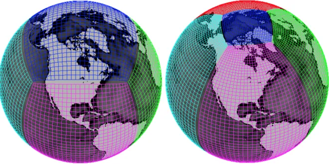
As in the ECCO framework, ECCO LLC270 is based on a global ocean and sea-ice permitting configuration of the Massachusetts Institute of Technology general circulation model (MITgcm, Marshall et al. 1998). The grid employed is the LLC270 grid (see Summary). Fig. 1 (right panel) shows that LLC270 grid has five faces covering the whole globe, with simple latitude-longitude grid between 70°S and 57°N and an Arctic cap (Forget et al., 2015). The dimensions for the Lat-Long faces are [810x270] and for the polar Cap is [270x270] (thus LLC270). The horizontal resolution varies spatially from 12km at high latitudes to 28km at mid-latitudes. The deepest ocean bottom is set to 6145m below the surface, with the vertical grid spacing increasing from 10m near the surface to 457m near the ocean bottom.

The ocean-ice state estimate synthesizes the MITgcm model with nearly all available ocean and ice observations since the era of satellite altimetry (post-1992). This allows for a coherent, physically-consistent reconstruction of the three-dimensional, time-evolving ocean and sea-ice state. The estimate uses the adjoint method to iteratively minimize the squared sum of weighted model data misfits and control adjustments (Wunsch et al. 2009, 2013).

Figure 1: Cube-sphere grid (left) for ECCO CS510 and LLC grid (right) for ECCO V4 framework, including LLC90, LLC270, and up to LLC4320.

3. Observations

Remotely-sensed data constraints consist of: 1) daily along-track sea level anomalies from several satellite altimetry (Forget and Ponte, 2015) relative to a mean dynamic topography (Andersen et al., 2016), including TOPEX/Poseidon (1993-2005), Jason-1 (2002-2008),

Jason-2 (2008-2017), Geosat-Follow-On (2001-2007), CryoSat-2 (2011-2017), ERS-1/2 (1992-2001), ENVISAT (2002-2012), and SARAL/AltiKa (2013-2017), while Jason-3 and Sentinel-3 data are withheld; 2) monthly ocean bottom pressure anomalies from GRACE mass

concentration (Watkins et al., 2015); 3) daily sea surface temperature fields from passive microwave radiometry (Reynolds et al., 2002), including AMSR-E (2002-2010) and WindSat (2011-2017); 4) daily sea-ice concentration fields from SSM/I (Meier et al., 2017).

The primary in-situ data constraints include: the global array of Argo floats (Roemmich et al., 2009; Riser et al., 2016), shipboard CTD and XBT hydrography incorporated as

monthly climatological temperature and salinity profiles from the World Ocean Atlas 2009 (Locarnini et al., 2010; Antonov et al., 2010]), tagged marine mammals (Roquet et al., 2013, Treasure et al., 2017), and ice-tethered profilers in the Arctic (Krishfield et al., 2008).

4. Controls

The estimate iteratively adjusts the model controls to bring the model into consistency with the observations through ajoint model integrations (Wunsch et al. 2009, 2013). The model

controls include the initial temperature and salinity fields, the 3D parameters of Gent-McWilliam/Redi mixing scheme, and the time-varying atmospheric boundary conditions.

The initial conditions for T/S are from a 3-yr spin-up from WOA09; the initial GM/Redi mixing parameters are uniformly set to 100 m2/s; the first guess of the atmospheric forcing fields are taken from ECCO V4 (which are adjusted ERA-interim) except for the wind fields which are from original ERA-interim. The every 14-days time-varying adjustments to the atmospheric forcing include downward shortwave radiation, downward longwave radiation, precipitation, 2-m air te2-mperature, 2-2-m specific hu2-midity, 10-2-m zonal and 2-meridional wind. The di2-mension of the controls is over two billion, the same order of magnitude as ECCO CS510 reported by Schwedes et al. 2018. With planned extension, the control number will increase further.

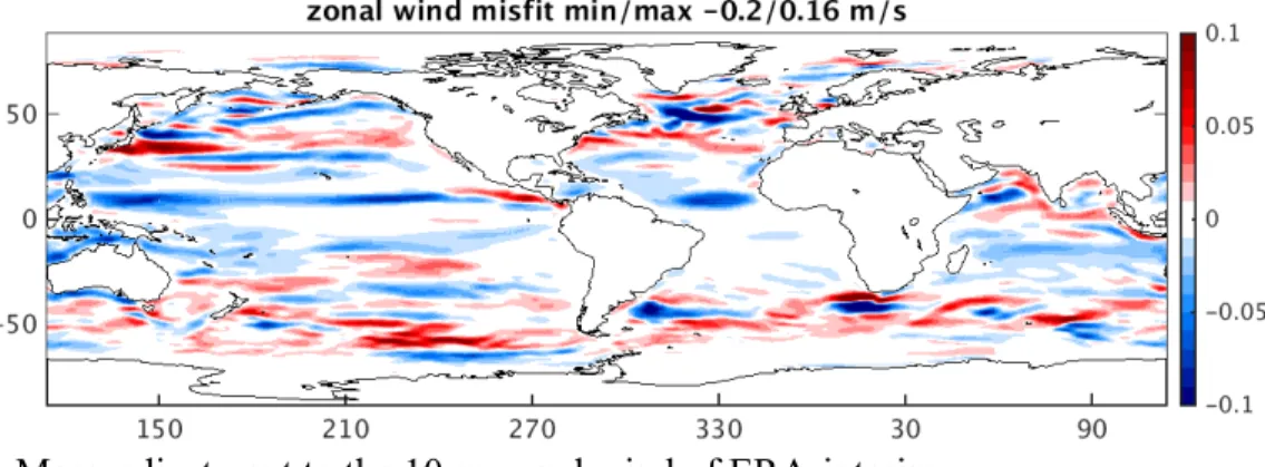
As an example, Fig. 2 shows the mean adjustment of zonal wind to ERA-interim over 1992-2017. Through fitting to oceanic data, in Equatorial the wind is weakened; in Southern Ocean the wind is generally strengthened; yet in mid-latitude the adjustment is mixed.

Figure 2: Mean adjustment to the 10-m zonal wind of ERA-interim.

5. Results

The ECCO LLC270 solution as of iteration 45 is available for download at

ftp://ecco.jpl.nasa.gov/Version5/Alpha/. Different aspects of this solution are illustrated in a suite of figures (so-called standard analysis plots) available for detail examination at

ftp://ecco.jpl.nasa.gov/Version5/Alpha/LLC270_overview_92_17.pdf and can be compared with equivalent atlas, like the one generated by ECCO-V4R3

ftp://ecco.jpl.nasa.gov/Version4/Release3/doc/standardplots.pdf. It includes model-data comparison, section transports, model states, budget analysis, and so on.

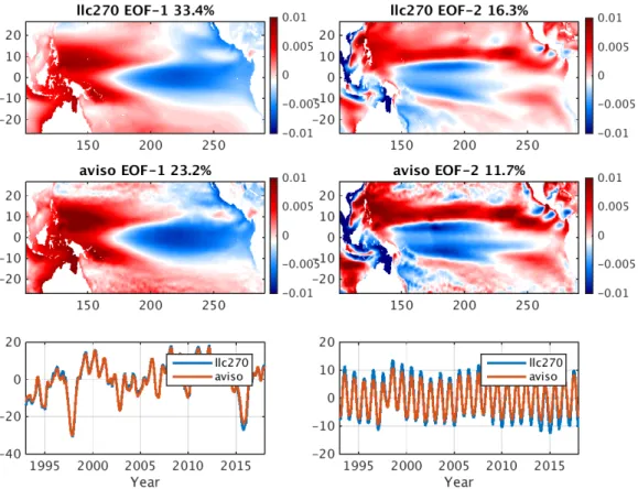
One interesting comparison between model and observation is to examine the gridded observation data, like the sea surface height anomaly provided by the Archiving Validation and Interpolatation of Satellite Oceanographic Data (AVISO; heep://www.aviso.altimetry.fr/) or the Roemmich-Gilson Argo Climatology (Roemmich and Gilson, 2009). Fig. 4 shows the first two EOF modes of the Pacific Ocean from 1993-2017 monthly mean SSH anomaly for LLC270 and AVISO. Clearly the model captures the SSH variability displayed by AVISO SSH data. The first

EOF mode exhibits a zonal dipolar pattern associated with interannual variability, and the second EOF mode presents a meridional tripolar structure varying on seasonal time scale.

Figure 4: The first two EOF modes of the Pacific SSH anomaly from LLC270 and AVISO over the time period of 1993-2017.

Not only does the model have a good agreement with the observation data, but also ECCO has more to offer. What ECCO LLC270, as well as other ECCO products provide, but the gridded AVISO product and other observational data sets (either discrete or mapped) do not, is the complete suite of ocean and ice variables that describes the entire physical state of the ocean and sea-ice (such as 3D temperature and salinity, 3D velocity, sea level, bottom pressure, and so on). In addition, ECCO product has advantage over most ocean reanalyses though they also provide comprehensive ocean fields. In contrast to most ocean reanalyses, the ECCO product fields, by design, are physically consistent with each other and with the air-sea fluxes, allowing for a full physical accounting of their temporal evolution fundamental to studies of attribution and causation.

Acknowledgement

This research was carried out in part at the Jet Propulsion Laboratory, California Institute of Technology, under a contract with the National Aeronautics and Space Administration.

References

Andersen O., P. Knudsen and L. Stenseng (2016), The DTU13 MSS (Mean Sea Surface) and MDT (Mean Dynamic Topography) from 20 Years of Satellite Altimetry. In IGFS 2014 (Cham: Springer International Publishing). 111–121.

Antonov J., D. Seidov, T. Boyer, R. Locarnini, A. Mishonov, and H. Garcia (2010), World Ocean Atlas 2009 Volume 2: Salinity. NOAA Atlas NESDIS 69, U.S. Government Printing Office, Washington, D.C.

The ECCO consortium (2018), Putting it all together: Enhancing the global ocean and climate observing systems with complete self-consistent ocean state and parameter estimates, in review by Frontiers in Marine Science.

Fenty I., D. Menemenlis, and H. Zhang (2015), Global Coupled Sea Ice-Ocean State Estimation. Clim. Dyn., doi:10.1007/s00382-015-2796-6.

Forget G. and R. Ponte (2015), The partition of regional sea level variability. Progress in Oceanography 314 137, 173–195.

Forget G., J. Campin, P. Heimbach, C. N. Hill, R. Ponte, and C. Wunsch (2015), ECCO version 4: an integrated framework for non-linear inverse modeling and global ocean state

estimation, Geosci. Model Dev., 8(10), 3071-3104, doi:10.5194/gmd-8-3071-2015.

Fukumori I., O. Wang, I. Fenty, G. Forget, P. Heimbach, and R. Ponte (2017), ECCO Version 4 Release 3, http://hdl.handle.net/1721.1/110380.

Khazendar A., I. Fenty, D. Carroll, A. Gardner, I. Fukumori, O. Wang, H. Zhang, H. Seroussi, D. Moller, B. Noal, M. Broeke, S. Dinardo, and J. Willis (2018), Jakobshavn's 20 years of Acceleration and Thinning Interrupted by Regional Ocean Cooling, accepted by Nature Geoscience.

Khazendar A., M. Schodlok, I. Fenty, S. Ligtenberg, E. Rignot and M.R. van den Broeke (2013), Observed thinning of Totten Glacier is linked to coastal polynya variability, Nature

Communications, doi:10.1038/ncomms3857.

Krishfield, R., J. Toole, A. Proshutinsky, and M. Timmermans (2008), Automated Ice-Tethered Profilers for Seawater Observations under Pack Ice in All Seasons. Journal of Atmospheric and Oceanic Technology 25, 2091–2105.

Liu J., K. Bowman, D. Schimel, N. Parazoo, Z. Jiang, M. Lee, A. Bloom, D. Wunch, C. Frankenberg, Y. Sun, C. O’Dell, K. Gurney, D. Menemenlis, M. Gierach, D. Crisp, A. Eldering (2017), Contrasting carbon cycle responses of the tropical continents to the 2015– 2016 El Niño, DOI: 10.1126/science.aam5690.

Locarnini R., A. Mishonov, J. Antonov, T. Boyer, H. Garcia, and O. Baranova (2010), World Ocean Atlas 2009, Volume 1: Temperature. NOAA Atlas NESDIS 68, U.S. Government Printing Office, Washington, D.C.

Marshall J., A. Adcroft, C. Hill, L. Perelman, and C. Heisey (1997), A finite-volume, incompressible Navier Stokes model for studies of the ocean on parallel computers, J Geophys Res-Oceans, 102(C3), 5753-5766, doi:10.1029/96jc02775.

Meier W., F. Fetterer, M, Savoie, S. Mallory, R. Duerr, and J. Stroeve (2017),

NOAA/NSIDC Climate Data Record of Passive Microwave Sea Ice Concentration, Version 3.

Menemenlis D., J. Campin, P. Heimbach, C. Hill, T. Lee, A. Nguyen, M. Schodlok, and H. Zhang, 2008: ECCO2: High resolution global ocean and sea ice data synthesis. Mercator Ocean Quarterly Newsletter, 31, 13-21.

Nakayama Y., D. Menemenlis, H. Zhang, M. Schodlok, E. Rignot (2018), Origin of Circumpolar Deep Water intruding onto the Amundsen and Bellingshausen Sea continental shelves, Nature Communication, doi:10.1038/s41467-018-05813-1.

Riser S., H. Freeland, D. Roemmich, S. Wijffels, A. Troisi, and M. Belbe´och (2016), Fifteen years of ocean observations with the global Argo array. Nature Climate Change 6, 145– 153.

Roemmich, D. and J. Gilson (2009), The 2004–2008 mean and annual cycle of temperature, salinity, and steric height in the global ocean from the Argo Program. Progress in Oceanography 82, 81–100.

Roquet F., C. Wunsch, G. Forget, P. Heimbach, C. Guinet, and G. Reverdin, G. (2013), Estimates of the Southern Ocean general circulation improved by animal-borne instruments. Geophysical Research Letters 40, 6176–6180.

Treasure A., F. Roquet, I. Ansorge, M. Bester, and L. Boehme, L (2017), Marine Mammals Exploring the Oceans Pole to Pole: A Review of the MEOP Consortium. Oceanography 30, 132–138.

Schwedes T., D. Ham, S. Funke, and M. Piggott (2018), Mesh Dependence in PDE-Constrained Optimisation, Springer, DOI 10.1007/978-3-319-59483-5.

Watkins M., D. Wiese, D. Yuan, C. Boening, and F. Landerer (2015), Improved methods for observing Earth’s time variable mass distribution with GRACE using spherical cap mascons. Journal of Geophysical Research: Solid Earth 120, 2648–2671.

Wunsch, C., P. Heimbach, R. Ponte, and I. Fukumori (2009), The global general circulation of the ocean estimated by the ECCO-Consortium, Oceanography, 22(2), 88-103,

doi:10.5670/oceanog.2009.41.

Wunsch, C. and P. Heimbach (2013), Dynamically and kinematically consistent global ocean circulation and ice state estimates. In: G. Siedler, J. Church, J. Gould and S. Griffies, eds.:Ocean Circulation and Climate: A 21st Century Perspective. Chapter 21, pp. 553–579, Elsevier, doi:10.1016/B978-0-12-391851-2.00021-0.