Dynamic response of human linearvection.

by

WILLIAM HON NING CHU

B.A.SC., University of Toronto 1973

SUBMITTED IN PARTIAL FULFILLMENT OF THE REQUIREMENTS FOR THE DEGREE OF MASTER OF SCIENCE

at the

MASSACHUSETTS INSTITUTE OF TECHNOLOGY February, 1976

Signature of

Author--Departmn of Aeronau cs and Astronautics October 3, 1975 Certified by

/

/

_{Thesis Supervisor} Accepted by

Chairan, Departmental Graduate Committee

Archives

JUN 9 1976

Nraas

q

I'

4

\~

ui

4

t

4

V 4 p I

d

by

WILLIAM H.N. CHU

Submitted to the department of Aeronautics and Astronautics on OCTOBER 3, 1975, in partial fulfillment of the reouirements for the degree of Master of Science.

ABSTRACT

The function of human visually induced sensation of linear motion (linearvection) was examined. The experiments performed were mainly designed to investiaate the frequency response of the human

linearvection mechanism. It was shown that both the

gain and phase exhibited steady decrease for increasing freauency. Asymmetry in response was also studied. It was shown that visually induced downward moving sensation was stronaer than the sensation of upward motion. There also seemed to be a stronger backward moving sensation than the forward one. The break frequency was found to be approximately 0.1 Hz.

Thesis Supervisor: Laurence P. Young Title: Professor of Aeronautics and

Astronautics

ACKNOWLEDGMENTS

The author wishes to express his gratitude to Professor Laurence R. Young whose patient advice and guidance permitted the realization of this research.

Thanks are also due Professor Charles M. Oman and Professor Renwick E. Curry for their valuable discussions and suggestions. The author also wishes to thank Mr. Alfred Chao for his cooporation in the early stage of this research. Technical assistance offered by Mr. John Tole and Mr. William Morrison provided significant contributions to the success of the experimental work.

Finally, the author expresses deep appreciation

to his wife, Grace, who without doubt carried the

greatest burden of graduate life. This thesis is dedicated to his wife and parents for their constant support and encouragement.

The research was supported by NASA grant NGR 22-009-701.

Chapter No. Page No. CHAPTER I INTRODUCTION

1.1 Background 8

1.2 Objectives of the Thesis 9

1.3 Results of the Thesis

1.3.1 Response to Constant Velocity stimuli 9 1.3.2 Linearvection Frequency Response to

Periodic Inputs 10

1.3.3 Linearvection Frequency Response to

Pseudo Random Inputs 12

1.3.4 Effects of Manual Pursuit Tracking 13

1.4 Outline of the Thesis 14

CHAPTER II EXPERIMENTS

2.1 Brief Outline of the Experiments 15 2.2 Experimental Facilities and

Organizations

2.2.1 Description of the Equipment 15

2.2.2 Experimental Organization 20

2.3 Experimental Software 23

2.4 Experimental Procedures

2.4.1 Static Case 29

2.4.2 Dynamic Case 33

CHAPTFP III ANALYSIS AND RESULTS

3.1 Cross Correlation Analysis and

Results 35

3.2 Fourier Analysis

3.2.1 Periodic Input 39

3.2.2 Pseudo Random Input 47

3.3 Asymmetrical Response 54

3.4 Effects of Manual Pursuit Tracking 55 4

CHAPTEP IV 4.1 4.2 Appendices A B C

CONCLUSIONS AND SUGGESTIONS FOP FURTHER PESFARCH

Summary of Human Linearvection Dynamics Suggestions for Further Pesearch

Operational Details of the Fxperiment Operational Details of the Data

Analysis Program Listinqs References

I

I

I

I

5

I

I

61 62

A

64 68 72 101

Fiaure No.

2.1

2.2

2.3

2.4 2.5 2.6,2.7, 2.8,2.9

2.10

2.11

2.12

3.1

3.2

3.3

3.4 3.5

Overview of Experimental Set up

Film Loop Motor Response to Dicitize

Inputs

Motor Linearity Curve

System Configuration for the

Experiment

System Configuration for the Data Analysis

Test Cases on Cross Correlation Coefficient Program

Bode Plot of a Known Transfer Function by the Digital Program FFTPLT

Typical LV Response to Pure

Sinusoidal Input

Results of Fast Fourier Transform Analysis of Signals Shown in

Fia.2.10 by Digital Program FFTPPT

Typical Subjective Response to

Hozontally Moving Stripes with

Constant Step Velocity.

Cross Correlation of Signals Shown in Fiq. 3.1

Summary of Cross Correlation Between Horizontal LV and the Constant Step Velocity Input

Typical Vertical LV Response to Pure

Sinusoidal Velocity Input

Harmonic Analysis d

6

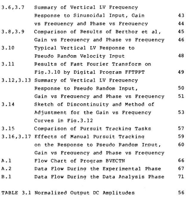
Page No. 16 18 19 21 22 25,26 27,28 30 31 32 36 37 38 40 42

3.6,3.7

3.8,3.9

3.10

3.11

3.12,3.13

3.14

3.15

3.16,3.17

A.1 A.2 B.1

Summary of Vertical LV Frequency Response to Sinusoidal Input, Gain vs Frequency and Phase vs Frequency Comparison of Results of Berthoz et al, Gain vs Frequency and Phase vs Frequency Typical Vertical LV Response to

Pseudo Random Velocity Input

Results of Fast Fourier Transform on Fiq.3.10 by Digital Program FFTPPT Summary of Vertical LV Frequency Response to Pseudo Random Input,

Gain vs Freguency and Phase vs Frequency Sketch of Discontinuity and Method of Adjustment for the Gain vs Frequency Curves in Fig.3.12

Comparison of Pursuit Tracking Tasks Effects of Manual Pursuit Tracking

on the Response to Pseudo Random Input, Gain vs Freguency and Phase vs Frequency Flow Chart of Program BVECTN

Data Flow During the Experimental Phase Data Flow Durinq the Data Analysis Phase

TABLE 3.1 Normalized Output DC Amplitudes

I

I

7

I

43 44 45 46 48 49 50 51 53 57 59 60 66 67 71 56

t

t

INTRODUCTION

1.1 Background

Flight simulation is always a compromise between

full six degree of freedom motion in the air and the limited motion in the laboratory. The purpose of this study is to examine the function of visually induced

sensation of linear self-motion, which may eventually be inteqrated with fixed based simulator motion to improve the fidelity of flight simulation and ride

quality.

Besides vestibular stimulation, visual cues also play an important role in man's judgment of his spatial position and orientation. Disorientation

arises when there is an incongruity between visual and

vestibular information. These conflicting visual and vestibular information are currently considered a main contribution to motion sickness.

Visually induced sensation of linear motion (linearvection) is easily illustrated by a common experience of sensing self-translation while noticing the movement of neighboring vehicle. The vestibular system, being acceleration sensitive, cannot help but let the visual system take over the task of motion

I

perception

in

a

constant

velocity

environment.

Self-motion effects have been studied in yaw, lateral

tilt

(Dichgan et al,1972),

pitch, roll, yaw (Young and

Oman 1974; Young, Oman and Dichgan 1975) and in linear

motion (Berthoz et al 1975).

Berthoz's

studies were

carried out in

the fore

and aft horizontal direction, whereas the goal of the

present

study

is

to

investigate

the

response

of

linearvection in the vertical direction.

1.2 Objectives of the Thesis

The objectives of the thesis are twofold:

(1) To

study

the

causal

relationship,

both

in

magnitude and in phase, between a static constant

visual stimulus and linearvection.

(2) To study the dynamic

response of linearvection

in

the presence of varying visual stimulus.

1.3 Results of the Thesis

1.3.1 Response to Constant Velocity Stimuli

The basis of the first part of the experiment is

the static phasic relationship between visual stimulus

and subjective motion perception.

The response latency

for

both

constant

vertical

and

horizontal

moving

9

holds for all stripe velocities up to 30 cm/sec which is about the maximun value, before saturation occurs,

for most of the subjects under the experimental condition described in detail in Chapter 2.

The word 'saturation' has two meanings in this

field. Firstly, it implies that the subject's visually induced sensation of motion is complete in the sense of possessing only self-motion and still

environment. Secondly, saturation suggests maximal visually induced sensation of motion. This definition certainly includes the first definition of saturation above. It is the latter definition which is implied

throughout this thesis.

Some subjects had slightly auicker response to increasing stripe velocity under saturation. However

this case does not occur frequently enough to render

the finding conclusive.

1.3.2 Linearvection Frequency Response to Periodic Inputs

The steady state subjective response to moving

peripheral field with sinusoidally varying velocity is generally periodic. The gain of the response decreases

as the frequency of stimulus increases. The result 10

4

(Fig. 3.6) shows an average drop of 11 db in gain in

the frequency range between 0.03 Hz and 0.8 Hz. The data exhibit strong agreement with those of Berthoz

(Fig. 3.8). However, Berthoz's result indicated gain greater than one for response to frequencies around

0.02 Hz. The lowest frequency used in this experiment

was only 0.03125 Hz. The significant difference between the present experimental condition and that of the Berthoz's is the direction of moving peripheral field. The horizontally fore and aft moving random

patterns were adopted by Berthoz while vertically up and down moving stripe patterns were used in this

experiment.

As expected, phase lag was observed to increase

as a function of frequency. Figure 3.7 illustrates the phasic relationship when the input visual

stripe-velocity is periodic in nature. The results agree with those of Berthoz in the frequency range

below 0.2 Hz. Also observed is the asymptotic characteristic of the phase lag which reaches a

limiting value about 60 degrees beyond frequency of

0.2 Hz. However, Berthoz's results (Fig . 3.9) showed

a steady increase in phase lag. Furthermore, the data

collected (Fig. 3.9) may even imply a possible

decrease in phase lag for frequencies greater than 0.5

11

data above 1.0 Hz can be gathered.

The harmonic analysis permits conclusions to be

made as to which subharmonics contribute the most to

the shape of the linearvection response to pure sinusoidal input. The results of the Fourier

transform (Fig. 2.11 and Fig. 3.4) clearly sugaests the strong presence of third harmonics. The synthesis

of the first and the third harmonics as illustrated in figure 3.5 confirmingly shows a great resemblance to typical responses. The emphasis of the third harmonics can be explained in terms of the typical subjective

sensations: the slow process of attaining linearvection and the sudden loss of it. The presence of other subharmonics were not found to be significant. However, three out of four subjects reported stronger down-moving sensation than up. The auantitative measure of this asymmetry is discussed in Chapter 3.2.

1.3.3 Linearvection Frequency Pesponse to Pseudo Pandom Inputs

The linearvection response to pseudo random stripe velocity is summarized in figure 3.12 and figure 3.13. Essentially, there is a steady drop in

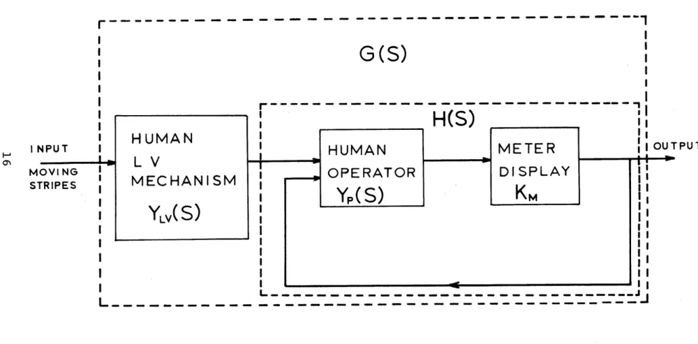
both gain and phase within the frequency range considered. However, two distinct features mark the

response as different from that of the periodic input.

Firstly, the gain is higher at low freqencies. Secondly, the phase lag exhibits steady increase.

As far as the ease of obtaining linearvection is concerned, pseudo-random stripe velocity was unanimously favored to be the best visual stimulus, even though the unpredictable nature of the

pseudo-random input made the magnitude estimation a

difficult task at times due to the high frequency

contents.

1.3.4 Effects of Manual Pursuit Tracking

Due to the inherent task of manual pursuit tracking in the experimental set up, the results obtained should be modified by taking off the pursuit tracking response. The results of correction to data

with pseudo-random velocity input were summarized in figure 3.16 and figure 3.17. In general, the effects

of manual pursuit tracking task were not very significant as far as altering the shape of the response curves is concerned. Hence, we can safely

claim that both the large phase lag and gain drop in

figure 3.12 and figure 3.13 were mainly due to the 13

I

1.4 Outline of the Thesis

The experiment is described in detail in Chapter 2. Hardware and software portion of the experiment

were considered separately. In Chapter 3 the experimental results are analyzed and discussions are made about the dynamic response of linearvection in the vertical direction. Finally, in Chapter A the conclusions of the thesis are stated and some

suggestions for futher work are made. Appendix A and B describe the operational details of the experiment.

CHAPTER II EXPERIMENTS

2.1 Brief Outline of the Experiments

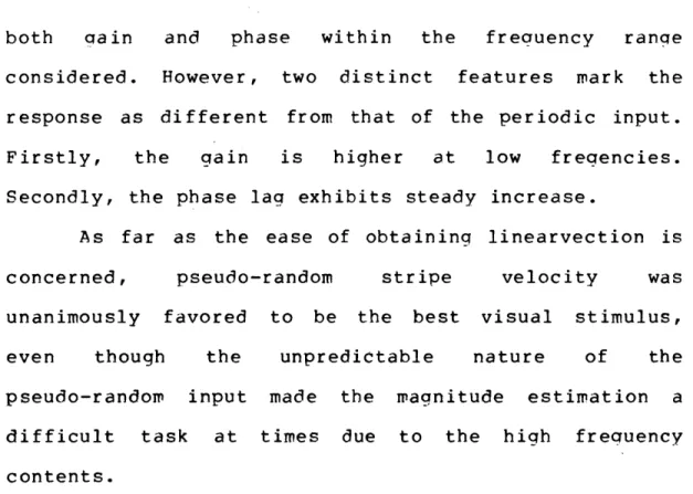
The basic experimental setup is illustrated by a simple block diagram shown in figure 2.1. The human

subject is divided functionally into two blocks. The block of human linearvection generator was in essence what this thesis strived to find. The inputs to this block were visul moving stripes which were made by

projecting a moving film loop onto the side windows of the Link trainer in which the subject was seated. To

report the linearvection, the subject was instructed to move the proportional, spring restrained control stick accordingly. The control stick was made in turn to drive a meter which provided visual feedback in order to increase the accuracy of such a method of magnitude estimation. The data were stored on analog tape and processed at the end of the run. The system input was provided and sequenced digitally by the PDP-8 computer.

2.2 Experimental Facilities and Organization

2.2.1 Description of the Equipment 15

r

I

SI---H

H(S)

MFTFR

|11OUTPUT

FIG. 2.1 OVERVIEW OF EXPERIMENTAL

SET UP

0*

*as

.

G (S)

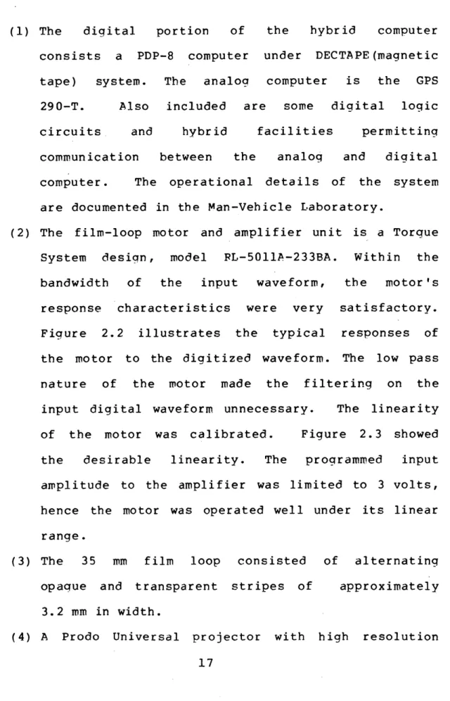
(1) The digital portion of the hybrid computer consists a PDP-8 computer under DECTAPE(magnetic

tape) system. The analog computer is the GPS 290-T. Also included are some diqital loqic circuits and hybrid facilities permitting

communication between the analog and digital computer. The operational details of the system

are documented in the Man-Vehicle Laboratory.

(2) The film-loop motor and amplifier unit is a Torque System design, model PL-5011A-233BA. Within the bandwidth of the input waveform, the motor 's

response characteristics were very satisfactory. Figure 2.2 illustrates the typical responses of the motor to the digitized waveform. The low pass nature of the motor made the filtering on the input digital waveform unnecessary. The linearity of the motor was calibrated. Figure 2.3 showed the desirable linearity. The programmed input amplitude to the amplifier was limited to 3 volts, hence the motor was operated well under its linear range.

(3) The 35 mm film loop consisted of alternating

opaque and transparent stripes of approximately 3.2 mm in width.

(4) A Prodo Universal projector with high resolution 17

J

-

--Ijj

H

9-

-C

Digitized

Wave-form, input to

the film loop motor

a

I

Filtered version of the above

0

₄

0

A

Film Loop Motor

Response, Signal

from Motor Tach

Feedback

g

0

Figure 2.2 Film Loop Motor Response to Digitized Input.

0

18

0

0

100 VELOCITY (CM/SEC) 90 80 70 60 50 40 30 20 10 -10 -8 -6 -4 2 4 6 8 10 -10 VO LT -20 -30 -40 -50 -60 -70 -80 -.- 90 -100

FIG.2.3 LINEARITY OF THE FILM-LOOP MOTOR; WINDOW STRIPE VELOCITY VS INPUT VOLTAGE TO THE FILM-LOOP MOTOR AMPLIFIER.

4

lens was used.

(5) The GAT-1

Link trainer was the simulator in which

the subject was seated. The film loop transport

and projector were mounted on top of the trainer.

Through a series of prism and mirror arrangement,

images were projected onto the side windows of the

trainer. The width of the stripes was 80 mm in

width.

The

shortest distance from the subject's

eye to the side window was about 32 cm.

(6)

The control

stick was basically the model airplane

joystick made by the Rand Manufacturing Co. Inc.

(7) The Brush Mark 240 strip chart recorder displayed

all the inputs, responses and results.

(8)

A Sanborn model 2000 FM tape-recorder handled all

the storage of raw data.

2.2.2 Fxpeirmental Organizations

Figure 2.4 and figure 2.5 depict an overview of

the system configuration used in both the experiment

and data analysis. The seguencing of the experiment

was

completely controlled

by

the

hybrid

computing

facilities.

The digital computer was basically slaved to the

clock

on the

analog computer. The digital program

automatically

sequenced

through

a

predetermined

20

0

0

SYSTEM CONFIGURATION FOR THE EXPERIMENT.

.V 6 v

n

FM

RECC

TAPE

-RDER

STRIP CHART

RECORDER

-A/D----

- D/A

-FIG.2.5 SYSTEM CONFIGURATION FOR DATA ANALYSIS

00

0

f

0

'

0

a

[

ANALOG

COMPUTER

(AMPLIFICAT ION, FILTERING etc.)

GPS

290 T

DIGITAL

COMPUTER

(CROSS CORRELATION, FAST FOURIER TRANSFORM)

DEC

PDP-8

TELETYPE

OUTPUT

0 0 _{Idb Am}

pattern of input waveforms. After D/A conversion, the

analog counterparts of the digital waveforms was fed

to the amplifier which drove the film-loop motor.

The subjective magnitude estimation on linearvection was represented by the analog signal created through the use of a control stick. The signals were then amplified on the analog computer and subsequently recorded on FM tape.

During the analysis phase, the data flow was reversed. The results of digital data analysis were outputed onto the Teletype machine, and/or D/A converted and displayed on the strip chart recorder. The details on the data flow and data manipulation were summarized in Appendices A and B.

2.3 Experimenral Software

Proqram BCP computed cross-correlation coefficient _pXY

X(k)Y(k+T) - X(k)Y(k)

I__TT)

-2

2

-2(21

X(X (k) -X (k) 2(Y (k)-Y(k)

T=1,2,...,9 sec between X(k) and Y(k) being the film speed and response to perceived LV respectively. The best fitting time delay was chosen to be the which gave

the maximun coefficient. This program was also written

to be real-time executable.

To demonstrate this program, two signals (Fig.

2.6) with known cross correlation were processed. The

resulting cross correlation was as expected and shown in figure 2.7. Since cross correlation coefficients

6

were actually computed, theoretically the amplitide and bias of the signal should have no effect on the

final coefficients. This fact was also satisfactorily

6

demonstrated by processing signals (Fig. 2.8) with different amplitude and bias. The results shown in

figure 2.9 were very similar to those shown in figure

0

2.7.

Program BVECTN controlled the sequencing and timing of calibration, pure sinusoidal input and

0

pseudo random input. The capability of repeated

calibration as well as calibration at random time was

implemented into the program through the use of sense

lines. Pure sinusoidal inputs were calculated internally in this program.

BRAND was called from BVECTN. This routine generated the pseudo-random inputs by summing up the

same number of sinusoidal signal used in BVECTN.

FFTPLT performed Fast Fourier Transform on both

6

the input and LV response signals. The results were 24

0 0 @

5

sec

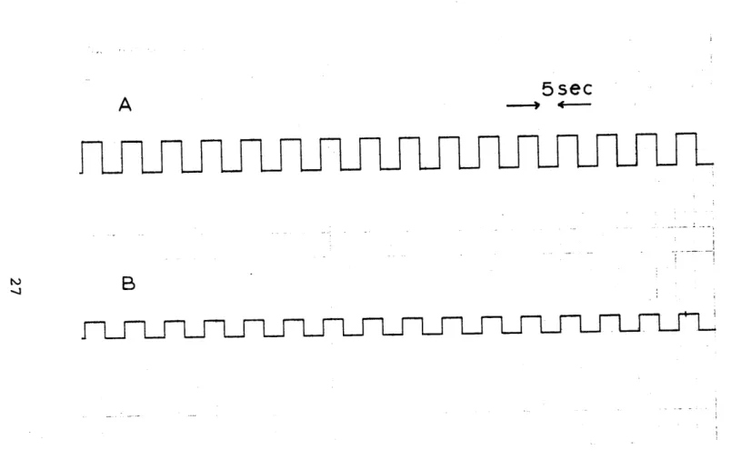
FIG.2.6 ZERO-MEAN AND EQUAL-AMPLITUDE SQUARE WAVES TOBE

CROSS CORRELATED.

Uj

THEORETICAL

FIG.2.7 RESULTS OF CROSS CORRELATION OF TWO SIGNALS SHOWN IN FIG.2.6.

0~ a

DELAY

CROSS

CORRELATION

TIME

COEFFICIENT

T(SEC)

exY

0 0.99 1 0.62 2 0.24 3 -0.14 4 -0.52 5 -0.90 6 -0.72 7 -0.34 8 0.04 9 0.36

1.0

0.8

0.6

0.4

0.2

0

-0.2

-0.4

-0.6

-0.8

-1.0

5

8

9

zc

a a a

0

0

0

5sec

A

-

-FIG. 2.8 SIGNALS TOBE CROSS CORRELATED;(A) ZERO MEAN

(B) BIAS.

1.0

DELAY CROSS

CORRELATION

TIME

COEFFICIENT

T(SEC)

exy

0 1.00 1 0.61 2 0.20 3 -0.19 4 -0.57 5 -0.93 6 -0.73 7 -0.28 8 0.18 9 0.57 THEORETICAL

1

2

5

8

9

FIG.2.9 _{RESULTS OF CROSS CORRELATION OF TWO SIGNALS SHOWN IN FIG. 2.8.}

0 0' 0 0 0 0 S

a

'a

0.8

0.6

0.4

0.2

0

-0.2

-0.4

-0.6

-0.8

-1.0

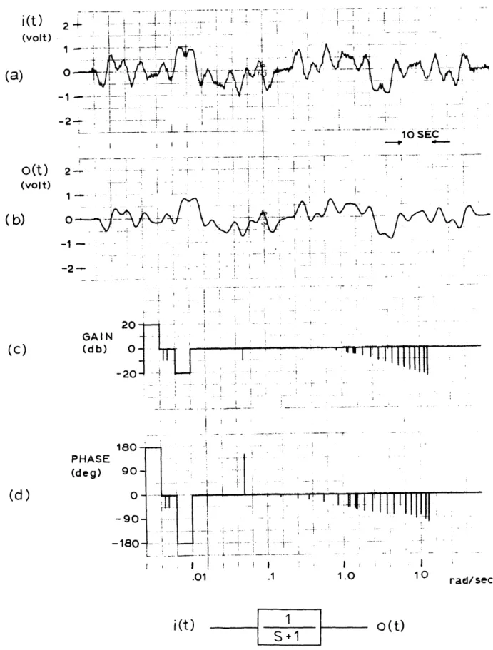
a a 'db

plotted on the strip chart recorder in terms of Bode

diagrams. The reliability of the program can be judged by its performance on a pair of input, output signal with known transfer function. Figure 2.10 illustrated such an example. The Bode plot was basically as expected and hence the working condition of the program was assumed.

FFTPPT performed only Fast Fourier Transform on the signals. However the amplitude and phase information of the subharmonics were printed out on the Teletype. Bode plot information can thus be

obtained manually from the results. Fiqure 2.11 showed

a typical result from analysing a response to pure sinusoidal input. Figure 2.12 gave a representative output from an analysis on pseudo-random input.

The details of these digital programs can be found in Appendix A and B.

2.4 Experimental Procedures

2.4.1 Static Case

Six subjects were exposed to a series of constant velocity visual field motion steps and asked

to move the control stick according to the amount of perceived LV. The visual field motion was in the

2+-1

- -1-- -2-10 SEC LL -F-.-,-. 2 -1

~

-1- -2-GAIN (db) 20 0 4. PHASE (deg)

(d)

180- 90-0 -90 -180 .01 .1 1.0 10

i(t)

1

o t)

s+1

FIG. 2.10 BODE PLOT OF A KNOWN TRANSFER FUNCTION BY THE DIGITAL PROGRAM FFTPLT.(a) INPUT WITH VAN HOUTTE'S SPECTRUM( REF.10 ) (b)OUTPU T (c) GAIN (d) PHASE

30

|(t)

(volt)

(a)

O(t)

(volt)

(b)

4

A

4

(c)

4

4

a

6

rad/sec

₀₁

6

01

--I

ST RIPE VELOCITY ₃₀ (c m/sec) f= --Lhz 64 0 -30 SUBJECTIVE VERTICAL LV RESPONSE: OUTPUT OF CONTROL STICK (volt)

f I t

m

T~i~-4

1

ik7~-f

I

'-=1

10 sec 3 -

-4

-3

I

_{I ,--}

f

--,* j

i

4~o~n 23 1

=INPUT

= 0.0000 F = 0.0456 2

=OUTPUT

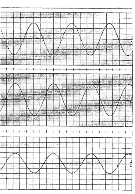
= 0.0000 F = 0.0151 = 0.0305 F = 0.0456 F = 0.0610 F = 0.0761 F = 0.1066 F = 0.1372 F = 0.1525 F = 0.2287 22 X2 A = 0.3271 A = 5.8691 A A A A A A A A A A -3 X2 0.9472 0.4638 0.5761 6.2695 0.3857 0.3759 0.3613 0.7031 0.3710 0.4492 0 = -180.00 0 = - 89.29 0 0 0 0 0 0 0 0 0 0 -180.00 -170-33 +178.06 -105.11 +132.45 - 1.49 +140.53 - 33.66 -102.91 + 31.28 F - FREQUENCY (HZ) A - AMPLITUDE 0 - PHASE (DEG)

FIG.2.11 TYPICAL VERTICAL LV RESPONSE TO PURE SINUSOIDAL VELOCITY INPUT (a) INPUT STRIPE VELOCITY COMMAND (b) SUBJECTIVE RESPONSE (c) FAST FOURIER TRANSFORM

RESULTS FROM DIGITAL PROGRAM FFTPRT.

31

(a)

(b)

(c)

o

-

- -

-z I

FFTPRT 1 =

INPUT

xz5 = 0.0000 A = 1.4697 0 = -180.00 F = 0.0151 A = 6.8359 0 = - 82.70 F = 0.0227 A = 6.8603 0 = +101.42 F = 0.0380 A = 6.8212 0 = - 71.19 F = 0.0532 A = 6.8896 0 = +116.54 F = 0.0837 A = 6.8115 0 = +131.74 F = 0.1296 A = 6.8701 0 = - 25.83 F = 0.1752 A = 6.7675 0 = - 3.07 F = 0.1831 A = 0.3173 0 = -179.12 F = 0.2136 A = 0.3271 0 = -165.32 F = 0.2211 A = 6.8798 0 = -160.31 F = 0.2822 A = 0.6884 0 = + 50.80 F = 0.3583 A = 0.6738 0 = - 93.33 F = 0.4499 A = 0.6835 0 = +133.85 F = 0.5568 A = 0.6542 0 = + 5.97 F = 0.6789 A = 0.6640 0 = -114.25 F = 0.8161 A = 0.6738 0 = +104.23 F = 0.9687 A = 0.6640 0 = -150.99 F = 1.1367 A = 0.6445 0 = +114.25 F = 1.3198 A = 0.6005 0 = -156.53 F = 1.5180 A = 0.5957 0 = +121.64 F = 1.7470 A = 0.5566 0 = + 54.66 F = 1.9147 A = 0.5371 0 = - 42.01 2

=OUTPUT

xz5 = 0.0000 A = 1.5087 0 = -180.00 F = 0.0151 A = 6.7968 0 = - 88.15 F = 0.0227 A = 6.7675 0 = + 92.98 F = 0.0380 A

=

6.6259 0 = - 84.90 F = 0.0532 A = 6.4941 0 = + 97.55 F = 0.0837 A = 5.9912 0 = +103.27 F = 0.1296 A = 5.2783 0 = - 65.74 F = 0.1752 A = 4.4970 0 = - 51.67 F = 0.2211 A = 3.9501 0 = +144.75 F = 0.2822 A = 0.3271 0 = - 11.95 F- FREOUENCY (HZ) g A - AMPLITUDE 0- PHASE (DEG)

FIG.2.12 RESULTS OF FOURIER ANALYSIS OF SIGNALS SHOWN IN FIG. 2.10 FROM DIGITAL PROGRAM FFTPRT.

horizontal fore and aft direction. The sequence of the

steps was designed to be random. Hence the results obtained by cross correlation method would be an

average time delay for all the possible step jumps.

2.4.2 Dynamic Case

Four subjects were used to take data in this part of the experiment. Firstly, the subjects were exposed to a number of constant step velocities for the training as well as the calibration purposes. They

were told the exact speed of the film under exposure. They were also instructed to move the control stick to

the appropriate relative position. This task was further assisted by the visible display meter which

corresponded to the control stick output, even though

the control stick is a spring-centered device. This

calibration and training procedure was repeated until

the subject could indicate the correct film speed without being told.

Calibration velocities were 30, 15 and 7.5

cm/sec in both up and down directions. Followinq the

calibration period, the subject was exposed to pure

sinusoidal inputs with different frequencies but same peak velocity namely 30 cm/sec. The order of the input

frequencies was chosen at random in order to minimize

the order effects. During the exposure to sinusoidal

inputs, the subject might be asked to track his LV(not

the stripe velocity) against the calibration speeds

again. This was done in order to see how strong the

habituation was if there were any.

Since it is desired to take data of steady state

response

and the time to reach

steady state varies,

therefore the duration of exposure for each frequency

differ

slightly.

The

end

of

exposure

for

each

frequency was determined when steady state response

was assumed

by judging from the response record being

produced from the strip chart recorder.

A pause of ten

seconds was taken between two successive frequencies.

One or two longer breaks were also taken within the

total experimental duration of about 45 minutes as it

0

might

be requested by the subject.

After all sixteen discrete sinusoidal velocities

were

given,

the

subject

was

exposed

to

the

pseudo-random velocity pattern. During the whole run,

the subject was instructed to faithfully indicate his

perceived velocity of self-motion rather than that of

the film stripes.

34

CHAPTER III

ANALYSIS AND RESULTS

3.1 Cross correlation Analysis and Results

To determine the LV delay in response to a constant step velocity input, real-time analytical

algorithm was developed. The scheme was based on the

application of the cross correlation coefficient

(equation 2.1).

However, inherent assumptions existed when equation 2.1 was adopted to compute the cross correlation coefficient. Mainly, the signals were assumed to be stationary and ergodic processes. The time invariant property was also implied. Figure 2.6 to figure 2.9 illustrated the use of this algorithm.

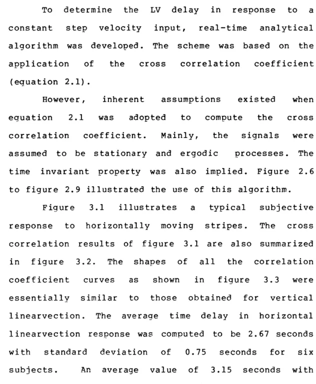
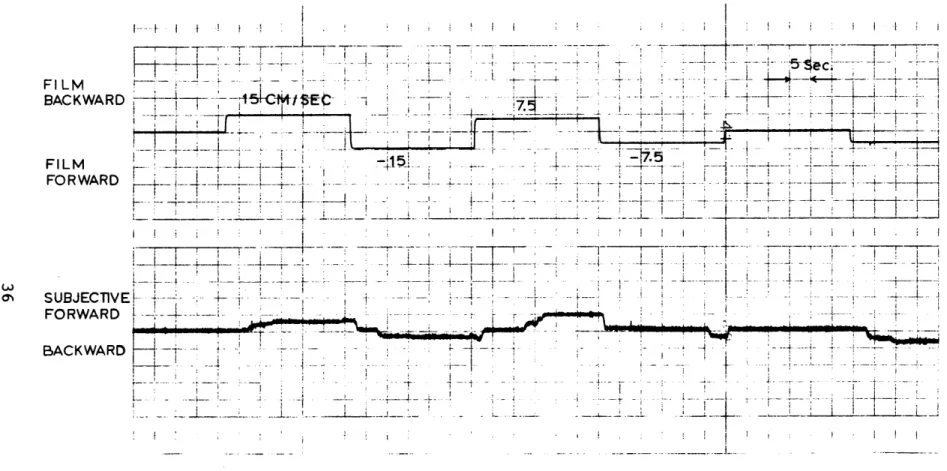
Figure 3.1 illustrates a typical subjective response to horizontally moving stripes. The cross correlation results of figure 3.1 are also summarized in figure 3.2. The shapes of all the correlation coefficient curves as shown in figure 3.3 were essentially similar to those obtained for vertical linearvection. The average time delay in horizontal linearvection response was computed to be 2.67 seconds with standard deviation of 0.75 seconds for six subjects. An average value of 3.15 seconds with

FI LM BACKWARD -f -$---

t

- - --FILM -41- -FORWARD -SUBJECTIVE' FORWARD _Jl BACKWARD i

-FIG. 3.1 TYPICAL HORIZONTAL LV RESPONSE TO MOVING STRIPES WITH

CONSTAN T STEP VELOC ITY.

w

W. U w _v

1.0

0.9

0.8

0.7

0.6

0.5

0.4

-J

0.3

0.2

0.1

0

0 0 0 0

00O

0

₀

O0

I

. .-. 1 .I . .

0

1

2

3

4

5

6

7

8

9

'

(SEC)

FIG.3.2 CROSS CORRELATION OF SIGNALS SHOWN IN FIG. 3.1.

DELAY CROSS

CORRELATION

TIME

COEFFICIENT

T(SEC) eXY 0 0.62 1 0.674 2 0.694 3 0.702 4 0.703 6 0.693 7 0.682 8 0.665 9 0.643

o

a w _w

4

0.9

DATA FROM 6 SUBJECTS

0.8-LL

OE

L-w

0

U

z

0

w

0

U

U) U)

0

0.61

0.5

0

1

2

3

4

5

6

7

8

9

DELAY TIME

(sec)

FIG.3.3 SUMMARY OF CROSS CORRELATION COEFFICIENT BETWEEN HORIZONTAL LV AND CONSTANT STEP VELOCITY INPUT.

standard deviation of 0.88 seconds was found for the

vertical linearvection response. Four subjects were used in the vertical case. Standard t-test performed on the two means showed that the difference was not

significant with significance level of 0.1.

3.2 Fourier Analysis

3.2.1 Periodic Inputs

The software used in this part of the analysis was mainly developed by Van Houtte, a former student

of the laboratory. Both the frequency components of

the input and response signals were analyzed. The Fast Fourier Transform technique involved in the analysis was basically the algorithm of Cooley and Tukey

(Ref.1, Pef.3).

Figure 2.11 illustrated a representative example. Figure 3.4 showed some more typical results.

Hand calculation had to be oerformed in order to obtain the gain and phase difference information. As

observed from these data, the input periodic signals were accurately analyzed, since other than some small

dc level, the only frequency component was the input

frequency. This performance of the computer software

again strengthened its reliability, and the results 39

4

STRIPE _30. V ELOCI T Y (cm/ sec) f = . z 0 30-SUBJECTIVE 3-VERTICAL LV RESPONSE: OUTPUT OF 0-CON TROL STICK (volt) -3-22 FFTPRT 1 =

INPUT

F = 0.0305 2= F= F= F = F = F A

0

4

4

I

4

A A

OUTPUT

0.0000 0.0151 0.0305 0.0456 0.0610 0.0915 0.1066 -2 x2 0.1513 5.9082 -2 x2 0.7470 0.6347 4.4824 0.4931 0.3271 0.3417 0.5029 0 = -180.00 0 = - 88.33 0 0 0 0 0 0 0

4

= -180.00 - + 83.84 = -103.18 = + 40.60 = - 35.33 = - 25.40 - + 64.16

I

I

FREQUENCY(HZ) AMPLI TUDE PHASE (DEG)

FIG. 3.4 TYPICAL VERTICAL LV RESPONSE TO PURE SINUSOIDAL VELOCITY OF FREQUENCY 1/32hz.

40

from the digital analysis would be more trustworthy.

The output response signals were in general

composed of many harmonics with varying amolitude. One

of the outstanding harmonics was the third harmonic

which had the greatest amplitude among all the other

harmonics. This observation led to the reconstruction of the shape of the linearvection response to sinusoidal input. The strong resemblance between the typical response and that of the reconstructed response by appropriately summing the first and third

harmonics as shown in figure 3.5 confirmed the

existence of a large third harmonics distortion in the

linearvection response to sinusoidal input.

Other harmonics contained substantially smaller amplitude than that of the third and were therefore not specially analyzed. However, all the frequency components other than the fundamental had to be

considered remnants of the linearvection response process.

The gain and phase difference for the fundamental frequency were computed for each subject and gathered together in figure 3.6 and figure 3.7 respectively. Averaged results across the four subjects were summarized in figure 3.8 and figure 3.9

in which the data from Berthoz et al (Ref.2 ) for the

1ST HARMONIC 0.03125 HZ 3RD HARMONIC 0.09375 HZ 1 ST+3RDHARMONICS TYPICAL VERTICAL LV RESPONSE TO 1ST HARMONIC

FIG.3.5 HARMONIC

ANALYSIS

42

01

4

10 SEC

41

4

6

6

/*O"\\

6

0

6

0

61

//O,***\

FREQUENCY (HZ)

0.1

_1.0

I I a ~ ~ * I I

~ ~

1

O

-0

x

X

X

0

FIG 3.6 VERTICAL LINEARVECTION; FREQUENCY RESPONSE TO MOVING STRIPES

WITH SINUSOIDAL VELOCITY; GAIN VS FREQUENCY .

4

2

0

GAIN

(DB)

001

I I U U U Nm

-2

-4

-6

-8

-10

-12

-14

-16

-18

-20

I

FREOUENCY(HZ)

0.1

I U I S U S I

1.0

X

0

FIG.3.7 VERTICAL LINEARVECTION: FREQUENCY RESPONSE TO MOVING STRIPES

WITH SINUSOIDAL VELOCITY; PHASE VS FREQUENCY.

0 0

0

0e

a

PHASE

(

0

)

40

20

0.01

0

-20

-40

-60

-80

-100

-120

-140

-160

-180

-200F

-a

I

I

I

I I

I

I

AD

e

~

T e 0 _F-1

FREQUENCY(HZ)

0-1

0

-2

-4

-6

-8

STRIPES WITH SiNUSOIDAL VELOCITY ; GAIN VS FREQUENCY.

GAIN

(DB)

4

2

1.0

I

TI

A-BERTHOZ(HORIZONTAL LINEARVECTION) O-MEAN OF 4 SUBJECTS I _

16

FIG.3.8 VERTICAL LINEARVECTION: FREQUENCY

Un

-10

-12

-14

-16

-18

-20

I

RESPONSE TO MOVING

40

PHASE

(o)

₂₀

FREQUEN

0.01

0-1

T

-20

T

-40

-60

I

4

0

o----*o

-80

1

-100

A- _{BERTHOZ (HORIZONTAL LINEARVECTION)}

-120

O-MEAN OF 4 SUBJECTS -+16

-140

-160

-180--200

CY(HZ)

1

w'

\T

{-4

I'

FIG.3.9 VERTICAL LINEARVECTION : FREQUENCY RESPONSE TO MOVING STRIPES WITH SINUSOIDAL VELOCI TY ; PHASE VS FRQUENCY.

similar experiments in the horizontal plane was also included.

3.2.2 Pseudo Random Input

Similar digital computer programs were used here to analyze linearvection response to pseudo random

velocity input. An added feature of the software was

the capability of plotting the Bode diagram directly onto the strip chart recorder. Neverthless, hand computations were also performed in getting the gain

and phase difference between the frequency components of the pseudo random input and those of the response. This redundant procedure helped to double check the complex software used. Again the fact that the Bode plots obtained by hand calculation were similar to those computed directly by the computer proved the consistency of the software.

Figure 3.10 to figure 3.11 displays a typical

vertical LV response to pseudo random velocity input

and the subsequent Fourier analysis by both digital programs FFTPLT and FFTPPT. The summary of the four subjects' results are shown together in figure 3.13

and figure 3.14.

Although there were limited instances when some subjects did not response to high frequencies during

(ai)

PSEUDO RANDOM VELOCITY INPUT (cm/sec) SUBJECTIVE VERTICAL LV RESPONSE (OUTPUT OF CONTROL STICK) (b) (volt) GAI N (db) 20T 0 -20 30 -t 0 3 I 1 O

~VV~~r

I

2KLi

I -1 ~ -PHASE 180-(deg) 0---- -

----1

6-6

-180 .01 1 1.0 10 r ad/ sec FIG.3.10 TYPICAL VERTICAL LV RESPONSE TO PSEUDO RANDOM VELOCITY INPUT (a) INPUT (b)SUBJECTIVE RESPONSE; (c)GAIN AND (d)PHASE OF BODE PLOT DONE BY

DIGITAL PROGRAM FFTPLT. 48

A

4

(C)

4

I

I

(d)

0

0

a

0

FF TPRT 1 =

INPUT

= 0.0000 F = 0.0305 F = 0.0456 F = 0.0761 F = 0.1066 F = 0.1677 F = 0.1982 F = 0.2592 F = 0.2897 F = 0.3508 F = 0.4423 F = 0.4729 F = 0.5644 F = 0.6254 F = 0.6560 F = 0.7170 F = 0.8085 F A

0

-4 x2 1.0156 3.3593 3.3691 3.3447 3.3837 3.3349 3.3886 3.3056 3.3935 0.3320 0.3320 0.3466 0. 3271 0.3320 0.3466 0.3271 0.3222 0 0 0 0 0 0 0 0 0 0 0 0 0 0 0 0 0 -180.00 - 76.11 +111.26 - 54.84 +139.74 +168.22 + 2.37 + 30.67 -154.42 + 74.79 - 66.44 +130.42 - 6.76 -159.43 + 35.24 + 66.09 - 75.14 FREQUENCY (HZ) AMPLITUDE PHASE(DEG)

2

=OUTPUT = 0.0000 F = 0.0151 F 0.0305 F = 0.0456 F = 0.0610 F = 0.0761 F = 0.0915 F = 0.1066 F = 0.1220 F = 0.1372 F = 0.1525 F = 0.1677 F = 0.1831 F = 0.1982 F = 0.2136 F = 0.2287 F = 0.2441 F = 0.2592 F = 0.2746 F = 0.2897 F = 0.3051 F = 0.3508 F = 0.3662 F = 0.3813 F = 0.4118 F = 0.4423 F = 0.4729 F = 0.5034 xz5 A = 3.6279 A = 0.4443 A = 6.1572 A = 4.2578 A = 1.2158 A = 2.9101 A = 1.2792 A = 2.7685 A = 0.4345 A = 1.0156 A = 0.9619 A = 2.2509 A = 0.8691 A = 2.1728 A = 0.5468 A = 0.3808 A = 0.7031 A = 2.5781 A = 0.6738 A = 2.4316 A = 0.8593 A = 0.5859 A = 0.5810 A = 0.6689 A = 0.3271 A = 0.3710 A = 0.4980 A = 0.3662 -180.00 - 56.68 - 77.43 + 79.45 + 66.88 -106.52 -130.16 + 94.30 +139.57 +126.56 -127.52 +108.98 - 27.15 - 59.76 - 58.18 - 77.43 + 34.18 - 50.97 +112.06 +137.72 +162.77 - 7.20 - 14.58 +176.66 - 40.07 - 99.84 + 48.16 - 94.57

FIG.3.11 RESULTS OF FAST FOURIER TRANSFORM ON SIGNALS IN FIG3.10; OUTPUT

OF DIGITAL PROGRAM FFTPRT .

4

GAIN

(DB)

2

0

-2

-4

-6

-8

-10

-12

-14

-16

-18

-20

FREQUENCY(HZ)

0.1

1-0

03

0-~~

0

0\

C

0/

FIG.3.12 VERTICAL LINEARVECTION: FREOUENCY RESPONSE TO MOVING STRIPES

WITH PSEUDO-RANDOM VELOCITY; GAIN VS FREQUENCY.

0'

0

0

Ba'

U,

C)

e

40

PHASE

( 0 )

20

0.1

- - - - E -w -r w A

FREQUENCY (HZ)

1-0

a II -I - - - I

0,-0

-20

-40

-60

-80

-100

-120

-140

-160

0

x \

0

FIG.3.13VERTICAL LINEARVECTION: FREQUENCY RESPONSE TO MOVING

STRIPES WITH PSEUDO-RANDOM VELOCITY ; PHASE VS FREQUENCY.

0.01

0

U, H

180

F

-200

t - II 1 i i v

e

_o

e

a

S~~

w

discrete sinusoidal inputs, the observation on responses to- pseudo random input increased those instances. In other words, some high frequency

components of the input did not appear in the response

signal. From the data collected, qualitatively the

probability of having no response to input frequencies

above 0.5 Hz was considered to be significantly large. For example, figure 3.11 showed this low-pass

phenomenon of a subject's response to pseudo random input.

Intuitively, this phenomenon might be explained by the inherent 2 to 3 second response delay as found in the static constant input. The variation of velocity input beyond 0.5 Hz was certainly within the

response delay time constant of the linearvection system.

Also observed from the gain versus frequency results were the discontinuities which occured at 0.359 Hz. A sketch of the phenomenon and the adjustment made was shown in figure 3.14. This phenomenon occured because of the fact that frequency

components equal and greater than 0.359 Hz had input amplitude ten times less than those of the lower frequency components. Such a high frequency identification 'shelf' is a standard practice in

o.359

FREQUENCY

(HZ)

N

'K

EXTRAPOLATION

P EXTRAPOLATED POINT FOR CONTINUITY. o DATA

A ADJUSTED DATA

FIG. 3.14 SKETCH OF DISCONTINUITY AND METHOD OF ADJUSTMENT FOR GAIN VS FREQUENCY CURVES

IN FIG.3.12.

53

GAIN

manual control(McRuer,1974). The adjustments were

done by the simple argument of continuity. Hence the

latter section of the Bode plot was shifted

accordingly to start at the point which was determined

by extrapolating the front portion of the curve. This

phenomenon, however, was not observed in the phase 4 versus frequency results.

3.3 Asymmetrical Response

A difference in sign and/or amplitude between the dc components of input and output signals would suggest a possibility of asymmetry in the vertical linearvection response.

The small dc components in the input command

signals was not originally intended. Even though this input dc bias was not detected on the strip chart recordings during the experiment, it neverthless

showed up after the Fast Fourier Transform. The g

slight bias in the input was possibly due to the

inherent noise in the amplifiers of the analog

computer. 0

If the LV responses to upward and downward

moving stripes were the same, then the response to the

input bias would appear in the output response signal 6 in an equal quantity. That is, the dc amplitude of

the output eauals that of input. However this was not the case as observed from the data summarized in Table

3.1 in which were tabulated the cuantities obtained by dividing the output dc amplitude by that of the

input. Standard hypothesis testing was done on the

data to determine how significant the output dc level was different from that of the input. The significance

level of 0.005 was obtained for three subjects and a value of 0.3 for the fourth subject who had reported occasional stronger upward moving sensation. However three subjects did consistently show that their

response to upward moving stripes was larger than that

of downward moving stripes. The dc level in the output signals plus the results of hypothesis test were confirmingly in agreement with what the three subjects had reported after the experiments.

3.4 Effects of Manual Pursuit Tracking Task

Inherent to the experimental set up was the task of manual pursuit tracking as illstrated in Fig. 2.1, Conventionally, the inputs to the human operator in a

pursuit tracking task are both displayed variables which consist of the target and the follower (Fig. 3.15). The task involved in pursuing the target is to

minimize the distance between the target and the 55

POSITIVE INDICATES DOWNWARD LV

Table 3.1 Normalized Output dc Amplitudes.

56

4

6

6

SUBJECT A B C D 1.37 8.23 3.44 -1.04 1.78 13.53 3.69 -0.61 2.25 11.26 4.58 1.92 o U 1.31 16.74 3.73 2.52 9.65 3.72 0.96 I-- (L10.51 _{8.13 2.53} 0 -8.62 2.06 7.07 1.81 18.44 13.11

0

0

0

6

TARGET

POSITION

DISPLAY

HUMAN

OPERATOR

CON TROL

FOLLOWER

(a)

LV(QUANTIFIED

(b)

FIG.3.15 COMPARISON OF PURSUIT TRACKING

(b) SUBTASK OF PURSUIT TRACKING IN EXPERIMENT; (a) CONVENTIONAL PURSUIT TRACKING.

57

follower. However, in the present experiment, the

inputs to the human operator were different. While one of the inputs was a physically displayed quantity,

the other variable was a purely imaginary quantity

which we shall label as quantified linearvection.

Assuming sufficient similarity of the two types of pursuit task, we shall identify the subtask of pursuit tracking in the experiment as the conventional pursuit

tracking and previous data (Ref. 5) collected for conventional pursuit tracking were subequently used.

We can now isolate the human linearvection mechanism from the overall response of the system by taking off the effects of manual pursuit tracking. Using the notation in Fig. 2.1 the human vertical

linearvection mechanism can be easily expressed as

g

Y (S)= G(s) LV H(s)

Data for H(s) were those of Elkind (Ref. 5). The

results of modification to the linearvection data were

summarized in figure 3.16 and 3.17. The amount of adjustment to G(s) was not very large and the basic

feature of the linearvection response remained the same. Especially, the large phase lag at high frequencies were not significantly altered as might be expected. Hence the contribution of the pursuit tracking task to the overall experiment was small.

58

0

0 w

FREQUENCY(HZ)

0.1

s-MEAN OF 4 SUBJECTS ±1d

A-CORRECTED MEAN VALUE

FIG.3.16 CORRECTION OF VERTICAL LINEARVECTION RESPONSE DUE TO MANUAL PURSUIT TRACKING;

PSEUDO-RANDOM INPUT; GAIN VSFREQUENCY.

4

2

GAIN

(DB)

0

-2

-4

-6

Un

1.0

-8

-10

-12

-14

-16

-18

-20

A

i>d

A qw mr

0

r

PHASE

(0)

20

_{FREQUENCY (HZ)}

0.1

1.0

0 0.01

-20

-40

6

TT

-60

6

-80

0T0

T

-100

-120--

- MEAN OF 4 SUBJECTS!1S A

-140 A _{- CORRECTED MEAN VALUE}

-160--180-

_{FIG.3.17 CORRECTION OF VERTICAL LINEARVECTION RESPONSE}

DUE TO MANUAL PURSUIT TRACKING;

-200-

PSEUDO-RANDOM INPUT; PHASE VS FREQUENCY.

CHAPTER IV

CONCLUSIONS AND SUGGESTIONS FOR FURTHER RESEARCH

4.1 Summary of Human LV Dynamics

This thesis serves to lay the groundwork for future studies in visual vestibular interactions. The

results obtained may also be used in future designs of flight simulators incorporating the use of peripheral

moving visual fields.

Firstly, an average of 2 to 3 seconds of

response time was found for the subjective response to

moving peripheral visual field with constant velocity. Secondly, when exposed to periodic sinusoidal velocity, the subject's response decreases with increasing frequency. Referring to figure 3.8, a

sharp drop in gain was observed for frequencies above

0.1 Hz. The phase of the response lags behind the

input. The phase lag increases also with increasing frequency. However, due to the predictable nature of

sinusoidal input, the phase lag levels off to

approximately 60 degrees.

Thirdly, the LV response to vertically moving

stripes with pseudo random velocity was- also found to

be frequency dependent in the following manner.

Similar to sinusoidal input, the gain exhibits a steady drop as freauency increases, However, the

responses to frequencies below 0.2 Hz were generally larger than those of sinusoidal response. A sharp

drop in gain was also observed for frequencies above

0.2 Hz. Overall, the phase lag was larger than those

of sinusoidal response. The striking difference was the continuing increase of phase lag above 0.2 Hz

which is the frequency for which the phase lag of the

sinusoidal response tends to start levelling off.

Fourthly, the subjects generally had a stronger induced subjective sensation of moving downward.

Although, quantitative data were not available, there

seemed to be also a larger induced subjective

sensation of moving backward for the peripheral visual field moving fore and aft in the horizontal plane.

Fifthly, the inherent task of manual pursuit tracking did not alter the result significantly. Hence we can claim that the conclusions made above

were in essence the dynamics of human linearvection

response.

4.2 Suggestions for Further Research

Similar to the study by Young and Oman (Ref.

13), experiments could be done in order to find out

62

the effects of head position on linearvection.

Assuming that otolithes were responsible for human's sensing of vertical linear motion, then it might be

found that the vertical LV response were maximum for both an erect and inverted head, since in these

orientations, the otolith would be the least sensitive

to vertical linear acceleration and hence minimum

visual and vestibular conflicts result.

Another important consideration for future work is the improvement of magnitude estimation method used

in indicating the subjective response.

Sinusoidal responses to frequencies above 0.8 Hz

also deserve further attention, since there seemed to

be a trend of decrease in phase lag for frequency above 0.8 Hz.

OPERATIONAL DETAILS OF THE EXPERIMENT

A.1 Digital Portion

To run the experiment for the vertical

linearvection, the following digital programs are used. Program BVECTN was listed in appendix C. Other

programs which were written by Van Houtte can be found in his doctoral thesis (Ref. 10).

(1) BVECTN: The program logic is clearly represented

by the flow chart shown in figure A.l. Program BRAND which generates the pseudo random signals is called from this program. BRAND was original written by Van Houtte. The only modification made was the change of

frequency components for the pseudo random signals.

For the period of computation set at 1/64 seconds, the basic frequency, as Van Houtte called it, is 0.015625

Hz. The frequencies which are only prime multiples of

the basic frequency were used. The prime numbers chosen were 2,3,5.7.ll13,17,l9,23,29,3l,37,4l,43,47 and 53. These numbers should replace those numbers starting at location 600 to 617 in program BRAND. Sense line bit zero was used to control the arbitrary

termination of each frequency exposure. Also it was used to shorten the wait routine if desired. Sense

4

line bit one was implemented for the flexibility of

having calibration at any time.

(2) BRAND: This program was well documented in Van Houtte's doctoral thesis. Also needed in this program

is the routine which computes the sine of an angle. I This routine was also contained in Van Houtte's work.

A.2 Analog Portion

Basically the command signals computed by the

digital programs were amplified on the analog computer

in order to have a maximum voltage of 3 volts which £ corresponds to about 30 cm/sec of stripe velocity.

Subjective response signals in terms of control stick

voltage output were also adjusted so as to give peak

magnitude of 3 volts. Both input and output signals were further reduced by half and then recorded on FM

tape. The diagram in figure A.2 summarizes the

details of the data flow.

65