HAL Id: hal-01743641
https://hal.univ-cotedazur.fr/hal-01743641
Submitted on 27 Mar 2019
HAL is a multi-disciplinary open access
archive for the deposit and dissemination of
sci-entific research documents, whether they are
pub-lished or not. The documents may come from
L’archive ouverte pluridisciplinaire HAL, est
destinée au dépôt et à la diffusion de documents
scientifiques de niveau recherche, publiés ou non,
émanant des établissements d’enseignement et de
A fine-grained response time analysis technique in
heterogeneous environments
Guillaume Urvoy-Keller, A. Hafsaoui, A. Dandoush, M. Siekkinen, D. Collange
To cite this version:
Guillaume Urvoy-Keller, A. Hafsaoui, A. Dandoush, M. Siekkinen, D. Collange. A fine-grained
re-sponse time analysis technique in heterogeneous environments. Computer Networks, Elsevier, 2018,
130, pp.16 - 33. �10.1016/j.comnet.2017.11.006�. �hal-01743641�
A fine-grained response time analysis technique in
heterogeneous environments
A. Hafsaouia, A. Dandoushb,∗, G. Urvoy-Kellerc, M. Siekkinend, D. Collangee aEurecom, 2229 route des cretes , BP 193F-06560 Sophia-Antipolis, France
bESME-Sudria, Paris sud, 38 rue Moliere, 94200, Ivry sur Seine, France cLaboratoire I3S CNRS/UNS UMR 7271 06903 Sophia-Antipolis, France
dAalto University School of Science and Technology, Finland
eOrange Labs, Immeuble AGORA 905 rue Albert Einstein, 06921 Sophia-Antipolis, France
Abstract
Ii is crucial for the network operators and Internet service providers (ISPs) to deter-mine the reasons that cause large response time fluctuations. In this paper, we consider passive measurements from heterogeneous environment (ADSL, FTTH and 3G/3G+ access technologies) of an European ISP ‘Orange’. Through experimental analysis of real traces, the need of a fine-grained traffic analysis technique is demonstrated. We show that finding the root causes of the observed poor performance using simple met-rics such as response time, RTT and packet loss is difficult. In view of this fact, the different factors that play a role in determining the resulting response time are described through examples. Then, a breakdown method that drills down into the passively ob-served TCP connections is proposed. The method decomposes the end-to-end response time into many time periods and maps each one to a specific parameter or a physical phenomenon. Thus, the impact of not only the network parameters but also the ap-plication configuration and user behavior is captured. The resulting time periods are given as input to a clustering algorithm in order to group together transfers with simi-lar performance holding traffic of different application protocols over different access technologies. As a result, the contribution of each participant in the performance bottle-neck is identified. The proposed technique is validated through extensive simulations and real passively measured traces and it is compared to other works. Exemplifying the technique on real traces from Internet and enterprise traffic is introduced and dis-cussed to demonstrate the power of the approach and its simplicity. In contrast to some existing tools, ISPs and enterprise administrators do not need to modify their network architecture or to install a new software or a plugin at the client or at the server side in order to use our technique. In addition, data sampling is not used. This is particularly important in order to keep data consistency and to detect metrics peaks. Last, our tool deals with both long and short TCP connections.
Keywords:
∗Corresponding author
Traffic analysis, Root cause analysis, TCP, Performance evaluation, Internet traffic, Enterprise traffic, Clustering
1. Introduction
Internet Service Providers (ISPs) have a continuous need to measure the offered services and to enhance the performance perceived by their customers. In fact, poor performance does not always mean that the network is to be blamed. This fact particu-larly makes application-level performance monitoring problematic for the ISPs. Recent works(e.g. [1, 2] ), have shown that the Quality of Service (QoS) measures like packet loss and throughput do not indicate for many of today’s applications anything about the cause of the poor performance perceived by users. Shorter the response time is, better the performance is for most of the nowadays applications. For example, it is shown in [3, 4] that the main Web Performance Bottleneck is latency and not the bandwidth ca-pacity. Therefore, studying the reasons of large response time is becoming increasingly important. In general, the poor performance can be due to one or more of the following factors: (i) the applications behavior at the servers and/or the clients side such as throt-tling sending rates, (ii) the congestion control mechanism of TCP protocol, (iii) and the heterogeneity of access technologies, namely ADSL, FTTH, Cellular and legacy Ethernet.
The purpose of this work, is to present a simple yet efficient visibility solution that can diagnose and troubleshoot the performance of TCP-based services. In fact, a key feature of our time audit technique is the ability to divide a TCP connection into certain slots of time using a break-down approach in order to eliminate application response time problems. It is able to deliver for each TCP-based service the classi-cal QoS indicators (cumulative distribution function CDF of packet loss, RTT as well as of throughput). Moreover, it provides a fine grained analysis of response time for capturing the root causes of the poor performance (e.g. application impact, user or server behavior, network problems etc.). Another important feature of our Time Audit technique is the transparency of its use in complex WAN and LAN architectures as it simply uses passively collected traces from any point in the network. The main motiva-tion is that the passive analysis does not have the overhead that active monitoring has. In addition, data sampling is not used as in some active or real-time approaches. This is particularly important in order to keep data consistency and to detect metrics peaks due to the presence of the whole traffic for a given period. The active tools such as NetFlow [5] introduced by CISCO are Router Based Analysis Techniques. These tech-niques allow granular on-time traffic measurements as well as high-level aggregated traffic collection that can assist in identifying excessive bandwidth utilization or unex-pected application traffic. It helps the network admin to understand what is happening in general in his/her network. However, these Techniques are hard-coded into the net-work devices, e.i. routers. It uses usually a slice of the netnet-work capacity for sending continuously statistics or full copy of data for every packets to an external server for doing the analysis. Thus more expensive resources at the routers, core links, and exter-nal computing unit are required. Thus, using our approach does not require to modify the networking infrastructure or to install additional software neither at clients nor at
servers sides contrary of most network and application performance solutions such as [6, 7].
Some related works [8, 9, 10, 11, 12] have focused on this problem and developed root cause analysis techniques that can determine the primary cause for the throughput limitation of a TCP flow from a passively captured packet trace. The novelty of our present work is that our technique is completely independent of both the applications and underlying PHY/MAC layer technologies. Our approach enables detailed profiling of short and long flows, unlike some previous work in this area such as [9, 8] that only discuss the case of long TCP connections. In addition and contrary to most of the related work, we address the problem for most of the access technologies and not only in a given context like in [13, 14]. The approach is general enough to be applicable for studying the impact of any application on the performance and not only for a particular application/service.
We exemplify the above techniques on traces collected on various access networks under the control of the same french ISP (Orange), enterprise traffic and also on a simulated traffic. Moreover, we underscore the limitation of classical techniques to pinpoint actual performance problem.
Last, pieces and preliminary results of this work have been appeared in the follow-ing conferences [15, 16, 17].
The new contribution in this work consists of (i) the in depth validation of the methodology, (ii) the application of the methodology to different network infrastruc-tures, (iii) the evaluation of interactive services for both Internet and enterprise net-works and (v) the comparison of the advantages and the limitations of our methodol-ogy with other known works. Also, we provide new materials (Flow charts, Tables, Sections) for the presentation of this complete work.
The remaining of this paper is organized as follows. In Section 2, the limitations of classical approaches to profile the performance of services is highlighted and the new performance metric is introduced. In Section 3, a new approach to address the problem is proposed and explained. In Section 4, an empirical validation of our key algorithms is provided. Section 5 is dedicated to analyze and discuss some results for interactive services. Related works are presented in Section 6 with a comparison between our methodology and other close works from the literature. Section 7 concludes our work.
2. Performance metrics
Response time is the performance metric that we focus on in this paper. By re-sponse time, we mean the delay between making a request and finishing receiving the response. Such a metric is often used to characterize application performance. That is why it is a particularly interesting metric for ISPs and application service providers to measure.
Given the number of different technologies used today to access the Internet, net-work characteristics and conditions are clearly among those factors. Also, netnet-work engineers observe that the core network is well provisioned and, in most of cases, it is not congested. Therefore, ISPs need to know the causes of ‘not acceptable delays’ to deal correctly with the problem. For this reason, response time is often complemented
with throughput, round-trip time (RTT), and packet loss measurements in order to gain further insights into the observed response time.
However, we will show in the next subsection that the classical QoS indicators (response time with RTT and packet loss) fail to completely capture the underlying root causes of the observed poor performance. Hence, a more systematic approach to such performance analysis is necessary.
2.1. RTT Estimation
The round trip time corresponds to the spent time between a sender transmitting a segment and the reception of its corresponding acknowledgement. This interval in-cludes propagation, queuing, and other delays at routers and end hosts [18].
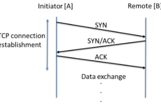
Several approaches have been proposed to accurately estimate the RTT from a sin-gle measurement point [19, 20, 21, 8]. To estimate RTT, we adopted two techniques. The first method is based on the observation of the TCP 3-way handshake [20]: one first computes the time interval between the SYN and the SYN-ACK segment, and adds to the latter the time interval between the SYN-ACK and its corresponding ACK. It is important to note that we take losses into account in our analysis. The second method is similar but applied to TCP data and acknowledgement segments transferred in each
direction1. One then takes the minimum over all samples as an estimate of the RTT.
For the present work, RTT estimation will be based on the second approach. 2.2. Response time analysis
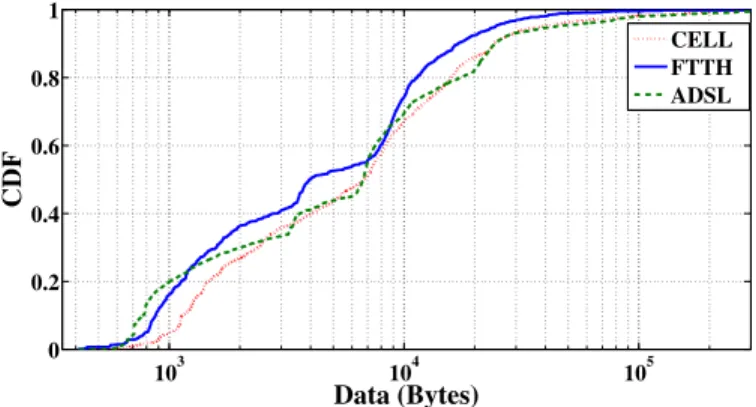
We exemplify the difficulty of interpreting the root cause of observed performance using simple metrics for the case of the Google search traffic extracted from real traces captured from ADSL, FTTH and 3G/3G+ access technologies of the ‘Orange’ Inter-net service provider. The description of the data-sets is presented in Appendix A. To identify the traffic generated by the Google search engine in the traces, we extract the TCP connections that transport HTTP requests containing Google tags in their HTTP header and exclude those to/from other services offered by Google like gmail, map, translate, etc. The used data set comprises of roughly 30K, 1K, and 6K connections for Cellular, FTTH, and ADSL traces, respectively. Given that TCP congestion control has a noticeable impact on transfer times of different sizes we want to see if the simi-larity of their connection size distribution was good enough to allow meaningful direct comparison. From Figure 1 that plots the CDF of the connections size, we see that the comparison is feasible.
Concerning the different network characteristics, Figure 2(b) plots the CDF of the estimated RTT for each connection from clients to Google servers over the different access technologies. The FTTH access offers very short RTT in general – shorter than 50 ms for more than 96% of connections. This finding is in line with the character-istics generally advertised for FTTH access technology. In contrast, the RTT for the connections using the Cellular access is notably longer than under ADSL and FTTH.
1Keep in mind that we focus on well-behaved transfers for which there is at least one data packet in each
103 104 105 0 0.2 0.4 0.6 0.8 1 Data (Bytes) CDF CELL FTTH ADSL
Figure 1: TCP Connection Size
To assess the impact of TCP loss retransmission times, we use an algorithm sim-ilar to the one developed in [22] to detect retransmitted data packets, which happen between the capture point and the server or between the capture point and the client. Table1 and Figure 2(a) reports the average packet loss rate, the average fraction of con-nections affected by losses events and retransmissions times for Google search traffic. We observe that Cellular traffic is characterized by the highest loss ratio and the highest fraction of connections affected by losses. The high fraction of connections experienc-ing losses in the Cellular case might be due to the random nature of errors in mobile environments such as interference.
Cellular FTTH ADSL
Packet loss rate 3.41% 0.56% 1.3%
Fraction of connections 24.75% 2.53% 5%
Table 1: Google loss rates
The observed RTTs and packet loss rate suggest that the response time over FTTH should be significantly shorter than the response time over ADSL. In turn, response time over ADSL should be remarkably shorter than the response time over Cellular access. The CDF plot shown in Figure 3 reveals that the ordering is correct but the absolute differences in response times between the different access technologies are not intuitive. The reasons are the application layer and the server behavior which are not properly reflected in the transport and network layer performance metrics. Therefore, in order to fully understand client perceived performance, we need a more systematic approach that uncovers all these factors.
2.3. Factors contributing to response time
We describe in this subsection the different factors that play a role in observed response time. These factors can be divided into two categories. Those that are caused by the various characteristics of the network belong to the first category. That category combines both the properties of the access link and the characteristics of the rest of the path. In the second category, we have all the factors that lie in the TCP end points.
102 103 104 105 106 0.8 0.85 0.9 0.95 1 0,756
Retransmission Times (Milliseconds)
CDF
CELL FTTH ADSL
(a) Retransmission Time per Connection
100 101 102 103 104 105 0 0.2 0.4 0.6 0.8 1 RTT (Milliseconds) CDF Cellular FTTH ADSL (b) RTT Estimation
Figure 2: Immediate Access Impacts
102 103 104 105 106 0 0.2 0.4 0.6 0.8 1
Response Time (Milliseconds)
CDF
Cellular FTTH ADSL
These include behavior of the transport protocol, all the application layer phenomena, and the user impact.
Network TCP end point
TCP protocol Application User
Capacity Sender buffer size Rate throttling Thinking time Available bandwidth Receiver buffer size Server load Usage patterns
RTT TCP congestion ctrl Content adaptation
Table 2: Factors influencing response time.
We list all the major factors in Table 2. Note that while the factors pertaining to the network apply to the entire TCP/IP path, often the access link contributes the major part of it, especially for the capacity and the RTT. Lack of available bandwidth leads to packet loss which is known to increase the response time because packets must be re-transmitted.
TCP protocol may increase the response time in a couple of ways. A too small buffer size at either the sender or the receiver slows down the transfer rate by setting an unnecessary small limit, from the network’s perspective, to the number of outstanding packets for the TCP sender. Congestion control mechanisms of TCP may also be a rate bottleneck because of a too slow growth of the congestion window in certain cases. This bottleneck emerges especially with small connections that transfer only a few packets.
The application being used may impact the response time by limiting the rate at which data is being transmitted. Such rate limiting is very common with streaming applications, e.g. when a server transmits a multimedia stream data at a rate higher than stream bit rate but lower than the available bandwidth rate in order to conserve bandwidth. Another factor increasing the response time is the server “thinking time”. When a server receives a request, depending on the application or web service, it may need to contact back-end servers which help craft the dynamic content included in the response, which can sometimes take a relatively long time. This delay is something that web service providers, such as Google, make great efforts to minimize because it directly influences the user experience and indirectly the revenue [23]. Similarly, the user can inflate the measured response time through thinking time with persistent connections that span over multiple requests and responses.
Figures 4 and 5 depict time sequence diagrams of two real mobile video streaming connections over a 3G access. Figure 4 is a piece of YouTube streaming session where the client was receiving traffic in a “all-at-once” manner, i.e., at a rate of approximately five times that of the stream encoding rate. In that case, the bottleneck limiting the rate was the access link and the receiving application which is visible from the occasion-ally zero advertised window and retransmitted packets. Figure 5 shows another video streaming connections where the server throttles the sending rate to 1.25 times the en-coding rate after the initial fast buffering. In this case, it is the application that forms the bottleneck.
The obvious question is then how we can evaluate the extent to which each of these factors contribute to the overall response time. We explain our delay-breakdown technique in the next section, which aims at answering this question.
Figure 4: Piece of YouTube streaming connection where receiver and available bandwidth form the bottleneck.
Figure 5: Piece of DailyMotion video streaming connection where server throttles the sending rate.
3. Breakdown/Clustering approach
We introduce in this section a new analysis technique that enables to account for the factors listed in Table 2 while profiling the performance of TCP transfers with 3-way handshake and a tear down phase.
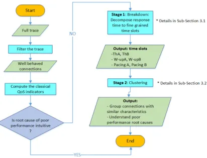
Figure 6: Illustrating the analysis methodology via flow chart
Figure 6 introduces the global methodology of our analysis technique via flow charts. In a first step, our approach computes the classical key performance indicators, e.g. connections size, loss, RTT, rate and application throughput, in order to charac-terize traffic and to show up main phenomena and trends. As a second step, which is
the subject of this section, if there is a need to go deep in the analysis, we are able based on capturing point in the network to extrapolate server responding time, client responding time, data transport time and a residual time. However, before perform-ing those two steps we may need to select a slice of the traffic, usperform-ing some meta-data from the transport/application layers (e.g. Fields from HTTP header), to be the input of our breakdown/clustering approach. This is what we called ”filter the trace“ in Fig-ure 6. In fact, some applications today rely on several parallel TCP connections as the case of the Web browsing where multiple connections are used to retrieve the different page objects. In such a case, performance degradation of some TCP connections (e.g., related to embedded advertisement) may be totally irrelevant for the user-perceived quality. Moreover, the initial filtering phase can be applied in order to focus the study on the performance of some specific application/service that suffers from performance degradation (e.g., e-mail). However, we can give all the trace as input to the approach as done in [24] (see Sec. C).
Let us now explain the second step of our approach that consists in turn of two stages. In the first stage, we transform, thanks to two successive breakdown steps (see Figure 8), each connection into a point in a 6 dimensional space, where each dimension can be related to some physical phenomenon or impact factor as shown in Table 3, e.g., the server data crafting time, access technology, routing and congestion avoidance algorithms, application configuration, and client behavior. In a second stage, we use a clustering approach to explore this multi-dimensional space. These techniques allow to assess if clusters, i.e., connections that experience similar performance, can be isolated and to characterize them.
Time slot dimension Warm-up A (resp. B) Theoretical A (resp. B) Pacing A (resp. B) Physical phe-nomenon or impact factor Corresponds to the time taken by the client (resp. the server), after receiv-ing the last data packet, before to perform (resp. to reply with) a data request (resp. re-sponse)
Is the duration that an ideal TCP transfer (RFC 2581) would take to trans-fer all the packets of the connection from the client to the server (resp. from the server to the client)
Is the remaining time from the subtraction of Warm-up and Theoretical periods from the total transfer time, for the client side (resp. for the server side). Pacing time is due either to the fixed capac-ity and available bandwidth of the path, where the access link is often the bottleneck. Also, network delay introduced by the line or network equipment, or some other mechanisms higher up in the proto-col stack, e.g., application imposing a rate limit.
Table 3: Definition of the 6 dimensions (time slots) and their relation to some physical phenomenon or impact factors
3.1. Stage 1: Breakdown
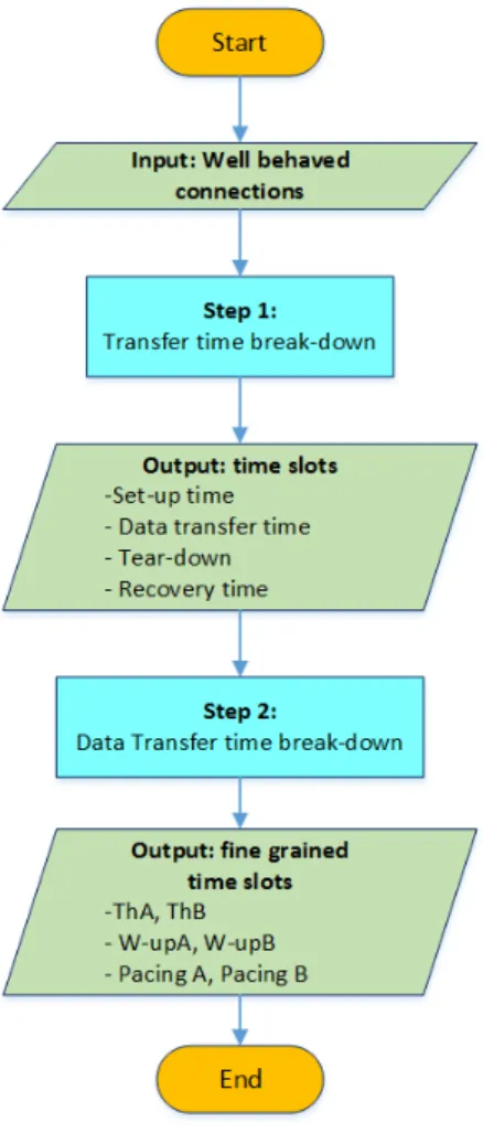
To illustrate this technique, we present in Figure 7 the corresponding flow chart. The overall breakdown technique consists of several steps and is illustrated in Figure 8. We explain each of these steps hereafter.
3.1.1. First step
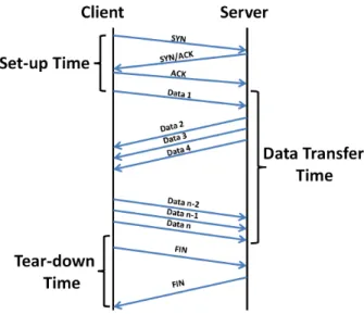
To understand the factors that affect the performance of TCP transfers, we first de-compose each transfer into three different phases, shown in Figure 9. This corresponds
Figure 7: Stage 1: Breakdown .
to Step 1 in Figure 8.
Set-up time is the time elapsed between the first control packet and the first data packet. Since we consider only transfers with a complete three-way handshake, the first packet is a SYN packet while the last one is a pure ACK in general. The connection set-up time is highly correlated to the RTT of the connection. For the Orange traces, the correlation coefficient are 42% for the Cellular trace, 30% for the FTTH trace, and 68% for the ADSL trace.
Data transfer time is the time elapsed between the first and the last data packet observed in the connection. It includes the loss recovery periods if the connection experienced packet loss.
Figure 8: Analysis process breaks the original trace down into different periods of time.
Figure 9: Transfer Time Break-Down
Tear-down time is the time elapsed between the last data packet and the last control packet of the connection. A well behaved connection in our terminology ends either with a FIN or RST. However, there can be multiple combinations of those flags at the end of a well-behaved transfer, which prolongs the tear down. Unlike set-up, tear down is not only a function of the RTT of the connection, but also a function of the application on top of TCP. For instance, the default setting of an Apache Web server is to allow persistent connection but with a keep alive timer of 15 seconds, which means that if the user does not post a new GET request after 15 seconds, the connection is closed. A consequence of the tight relation between the tear-down time and the application is a weak correlation between tear-down times and RTT in our traces: -1.5% for the Cellular trace, -0.5% for the FTTH trace, and 16% for the ADSL trace.
Recovery time is time spent by the TCP connection to recover from lost or cor-rupted packets, which is included in the data transfer time, as mentioned above. We compute it so that for a given transfer, each time the TCP sequence number decreases, we record the duration between this event and the observation of the first data packet whose sequence number is larger than the largest sequence number observed so far. Figure 10 illustrates a TCP connection suffering from packet loss. In this example, we count as recovery time the time elapsed between observing packets 7 and 8. To filter out reordering that occurs at the network layer, we discard each recovery period smaller than one RTT.
Figure 10: Recovery Time
3.1.2. Second step
Typical data exchange consists of trains of data packets flowing alternatively in each direction. The second step of our approach decomposes the data transfer time extracted during the first step into further components.
As we present in Figure 11, we term A and B the two parties involved in the transfer (A is the initiator of the TCP transfer and B is the remote side).
Figure 11: Initiator:A and remote side: B identification
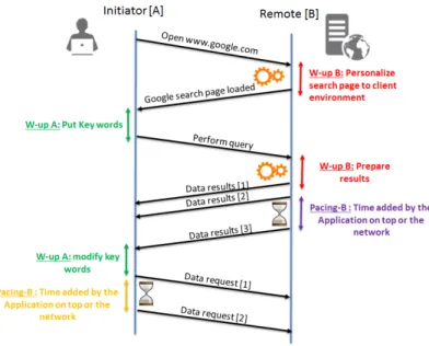
Our method breaks the entire data transfer time of each connection into a contigu-ous set of three types of periods: Warm-up time, Theoretical time, and Pacing time. Figure 12 illustrates these different periods for the case of a Google search transac-tion where A is a client of the ISP and B is a Google server.
Figure 12: Response Time Break-Down
Warm-up corresponds to the time taken by A or B before answering to the other party. It includes durations such as thinking time at the user side or data preparation at the server side. For the case of Figure 12, a Warm-up at A corresponds to the time spent by the client to type a query or to read the results returned by the server before issuing the next query or clicking on a link. A Warm-up of B corresponds to the time spent by the Google server to prepare the appropriate answer to the request.
Theoretical time is the duration that an ideal TCP transfer would take to transfer all the packets of the connection from A to B (or from B to A). It is an upper bound describing the best case behavior of a TCP connection having all the data available right at the beginning of the transfer and, furthermore, having an infinite path capacity. Thus, the transmission rate is limited only by the TCP slow start and the RTT between
A and B which we denote as RT TA−B (or RT TB−A). Following the example of
Figure 12, the client connects to a Google server, sends a query and receives the answer that fits into 3 data packets. As a result, theoretical times will be computed as the corresponding time spent according to a simple TCP model [25] with a given initial congestion window and 2 (resp. 4) data packets from the client to the server (resp. from the server to the client).
Once the time accounting for the Warm-up and Theoretical periods have been sub-tracted from the total transfer time, some additional time may remain. We term that remaining time Pacing time.
Note that to obtain accurate estimations of Warm-up, Theoretical and Pacing du-rations at the sender or the receiver side, we have to shift in time the time-series of packets received at the probe, hereafter called probe P. Specifically, we assume that a
packet received from A at probe P was sent RT TP −A
RT TP −B
2 in the future, where RT TP −A(resp. RT TP −B) is the RTT between P and A
(resp. B).
The above breakdown strategy results in a complete partition of the total transfer time. Let us revisit Table 2, which lists different factors that impact the response time and compare our data transfer time components to these factors. First, warm-up periods correspond directly to the user impact and application added delay, e.g., to generate dynamic content (especially under heavy load). Theoretical time accounts for the RTT and, to a certain extent, the TCP congestion control mechanism, but it completely neglects the bandwidth and capacity constraints and any application and user impact. Pacing time is due either to the fixed capacity and available bandwidth of the path, where the access link is often the bottleneck, or some other mechanisms higher up in the protocol stack, e.g., application imposing a rate limit.
Finally, as we presented in Section 2, for our performance analysis approach we focus on response time: the delay between a request and the response. According to our approach, we present in Figure 8 the sub-time composing the total response time. 3.2. Stage 2: Clustering
The second stage of our approach, presented in Figure 13, aims to group together connections with a similar data transfer time breakdown using clustering. This stage enables obtaining a global picture of the relation between the service, the access tech-nology and the usage.
After performing data transfer time break-down (Step 2 of Figure 8), each well-behaved connection is transformed into a point in a 6-dimensional space (Pacing, The-oretical, and Warm-up time of the client and the server). We use these six dimensions as a feature vector for each connection and use K-means to group connections with similar characteristics.
It is important to pay attention to the choice of the initial centroids and the number of clusters when using K-means.
First, to assess the number of used clusters, we rely on a visual dimensionality reduction technique, Distributed Stochastic Neighbor Embedding (SNE) [26]. t-SNE projects multi-dimensional data on a plane while preserving the inner neighboring characteristics of data. The application of this method enables to obtain 2D view – see Figure 19(a) – of the high-dimensional space, which enables to pick an appropriate value for the number of clusters. For the t-SNE function implemented in MATLAb, we set the default values of the perplexity parameter that is 30 as explained in the user guide [27] and we iterate 1000 times in order to reach a stable result. For more details about the impact of the tunable t-SNE parameters, in [28] the authors introduce several simple and comprehensive experiments in order to use t-SNE effectively.
Second, to address the problem of the choice of the initial centroids, we run the K-means Matlab implementation [29] 100 times, which is considered as a good prac-tice. By default, means uses the squared Euclidean distance measure and the k-means++algorithm for cluster center initialization. The k-k-means++algorithm uses an heuristic to find centroid seeds for k-means clustering. According to Arthur and Vassil-vitskii [30], k-means++improves the running time and the quality of the final solution. To enable a meaningful comparison between connections of different duration, we apply K-means on the average Warm-up, Theoretical and Pacing durations. Consider
Figure 13: Stage 2: clustering
again the case of Figure 12. Assume a similar connection performed by another user with two successive GET requests sent by the client instead of one (we assume a persis-tent HTTP/1.1 connection). If the two users experience similar performance on a per request basis, one would like that the clustering algorithm groups these connections together. This is achieved by a simple normalization approach (averaging procedure). We divide the total Warm-up and Pacing times by the number of trains (in each direc-tion) and the Pacing and Theoretical times by the number of packets (in each direction also).
To present results, we use boxplots2to obtain compact representations of the values corresponding to each dimension. On top of each cluster, we report the median size of the connections in this cluster, the cluster identifier and, if the connections originate from many traces, the percentages of connections per trace.
4. Empirical Validation
The main objective of this section is to validate our analysis methodology by sim-ulation and real traces provided by Orange. The Simsim-ulation is carried out under a Fedora Linux (kernel 2.6.22) environment, using the QualNet simulator [31]. QualNet is a commercial simulator based on GloMoSim developed at the University of Cal-ifornia, Los Angeles (UCLA). GloMoSim uses the Parallel Simulation Environment for Complex Systems (PARSEC). Qualnet generates TcpDump traces and has a simple graphical user interface. Throughout two different validation scenarios, we will show that our approach groups clients with similar profiles at the application (e.g. similar Warm-up or Pacing) or network layers (e.g. similar RTT) while capturing the root causes of long response time for TCP-based services. Table 4 summarizes the settings of two validation scenarios and the expected results from our analysis tool.
Scenario key settings Expected results and outcomes
1 Many classes of users who use 3 different applica-tions and get services running on remote servers in the same data center. One user class is penalized by a very short MSS size and some classes have limited user and/or server buffer sizes. Others have good settings and should experience a good perfor-mance.
Identify the root cause of the poor TCP perfor-mance experienced by some users. In other words, delineate users with performance bottlenecks and problems from an initial traffic mix (Isolate users with similar large pacing times).
2 Users of the same POP3 email service from the real Orange traces. The users use three different access technologies (3G+,FTTH & ADSL).
Our method should expose the same server think-ing time (Warm-up B) distribution regardless the access technology used by the users and should show the contribution of the access technology in the response time.
Table 4: Validation scenarios
For the simulation scenario, we consider the topology presented in Figure 14. It represents two sites: an edge site which consists exclusively of client machines with wired and wireless accesses to the network and a data center with application servers. On the two sites all appliances are inter-connected using a switch directly connected to a global router, which ensures inter-site connectivity. The description of the real data set used in scenario 2 and in the discussion introduced in the next section is reported in Appendix A.
For both scenarios, TcpDump traces are collected at the server side. Those traces are then uploaded via the Intrabase tool [32, 33] in the data base management system (DBMS) that we use to process traces collected in real network. A key advantage is
2boxplots are compact representations of distributions: the central line is the median and the upper and
lower of the box the 25th and 75th quantiles. Extreme values - far from the waist of the distribution - are reported as crosses.
Figure 14: Used Simulation Network
that we use exactly the same code to analyze and study the real traces and the synthetic ones.
4.1. First Scenario
In view of the fact that pacing time is related directly to two physical phenomena: (i) A bottleneck in the network and (ii) some other mechanisms higher up in the pro-tocol stack, e.g., sender/receiver buffer size. We will first consider in this scenario six classes of users corresponding to different application (HTTP, FTP, and Telnet) set-tings. Second, we penalized a class of users (number 4) by a very short MSS size (only 65 Bytes versus the default 1460 Bytes) and another class (number 6) by limited both client and server buffer size to 16KB instead of 64KB for the other classes as shown in Table 5. All the users benefit from the same network configuration. As we expect the results, we want to verify that the approach will correctly divide the response time and classify the users based on the perceived performance, and in particular based on the Pacing times.
users 1 users 2 users 3 users 4 users 5 users 6
Application FTP FTP TELNET TELNET HTTP HTTP
Connection Time (sec) 600 600 600 600 600 600
Bandwidth (Mbps) 10 10 10 10 10 10
Link Delay (ms) 30 30 30 30 30 30
MSS 1460 1460 1460 65 1460 1460
Sender Buffer Size 64500 64500 64500 64500 64500 16000
Receiver Buffer Size 64500 16000 64500 64500 64500 16000
Think Time (sec) - - - - 2 2
Table 5: User Classes
Figure 15 presents the clustering results using K-means and the projection obtained via t-SNE. The first observation here is that the clusters obtained with K-means are in good agreement with the projection obtained by t-SNE as indicated in Figure 15(b), where data samples are indexed using their cluster identifier in K-means.
Th B W−up B Pacing B Th A Pacing A 0 1 2 3 4 5 6
x 105Cluster 1= user 2−−Size datapkts A=50000−−Size datapkts B=0
Milliseconds
Th B W−up B Pacing B Th A Pacing A 0 2 4 6 8 10
x 104Cluster 2= User4, user 6 −− Size datapkts A=687−−Size datapkts B=687
Milliseconds
Th B W−up B Pacing B Th A Pacing A 0
500 1000 1500
Cluster 3= User 3, user5 −− Size datapkts A=687−−Size datapkts B=687
Milliseconds
Th B W−up B Pacing B Th A Pacing A 0
500 1000 1500
Cluster 4= user 2 −− Size datapkts A=50000−−Size datapkts B=0
Milliseconds (a) K-means Cluster 1 Cluster 2 Cluster 3 Cluster 4 (b) t-SNE
Figure 15: Heterogeneous Traffic: Data Clustering
Let us inspect the median size of the connections within each cluster, which is reported on top of each graph in Figure 15. We observe that two clusters gather the in-teractive traffic while the two other ones gather the bulk transfers. Indeed, Figure 15(a) shows that cluster 2 and 3 correspond exclusively to HTTP and TELNET connections while clusters 1 and 4 correspond to FTP traffic with median transfer size of 50,000 data packets. Cluster 1 corresponds to FTP connections characterized by large Pacing A value due to the limited receiver buffer size for users of class 2. Cluster 2 groups TELNET and HTTP connections with large Pacing A and B values: in fact users of class 4 were penalized by very short MSS size and users of class 6 by limited client and server buffer size. Let us now consider clusters 3 and 4. Those clusters correspond to shorter data transfer time break-down values. Cluster 3 groups Web and TELNET
connections that feature high Warm-up B as their MSS and sender/receiver buffer size are optimal. This means that when a connection is optimally tuned, the impact of processing times is more important than Pacing and Theoretical times. Cluster 4 cor-responds to FTP transfers with low Pacing A as those users have large sender/receiver buffer size.
Overall, we observe that our clustering method, when applied to a mix of con-nections with different parameters, identifies the root cause of poor TCP performance experienced by some users thanks to the fine grained analysis of the data transfer time (dividing it to six predefined slots).
4.2. Second Scenario
In this section, we consider a POP3 service that is implemented using the same set-up for the three different access technologies in the Orange traces, namely ADSL, Cellular and FTTH.
Figure 16(a) shows boxplots of 4 clusters obtained with Kmeans algorithm that are in good agreement with the projection obtained with t-SNE as indicated in the left plot of Figure 16(b).
Figure 17(a) depicts Warm-up B distribution for POP traffic. It shows approxima-tively the same Warm-up B distributions for identified clusters.
Based on the presented results in Figure 16(a), we can draw some conclusions for the main clustering parameters. We have seen that cluster 1 and 3 correspond exclusively to Cellular and FTTH connections, while cluster 2 and 4 group ADSL and Cellular ones. This first observation highlights the access impact for clustering results. Cluster 3 was identified by short Theoretical times A/B and null Pacing A and B. It shows that due to high throughput available in FTTH access, users are able to download data from POP3 server more faster than in ADSL and Cellular without Pacing values.
Figure 17(b) shows that cluster 4 presents the largest RTT, which in part explains the noticed Pacing A.
The CDF of Warm-up at server side reported in Figure 17(a) demonstrates that despite the diversity in access technology or in the cluster characteristics, our break-down technique is able to retrieve very similar distributions for all access technologies. Note that the three traces were not captured at the same time period and thus, the load conditions might explain the little differences observed in the CDF plots.
5. Results and discussion
In order to study the non-network parameters impact on the data transfer time that are often neglected in the literature, mainly servers/clients thinking times, we first ap-ply our fine grained response time analysis tool to the orange real traces presented in Appendix A for the case of typical key Internet service: google search. Second, we apply our methodology to a real trace collected from an enterprise network to study the performance of some internal policies and services. More precisely, we will study the LDAP protocol that is a key component in a number of interactive actions (login, mail completion, etc.) performed by the end users.
Th B W−up B Pacing B Th A Pacing A 0 500 1000 1500 2000 2500 3000
Size dpkts16−−Cluster 1−− CELL(%)=26−− FTTH(%)=0−−ADSL(%)=0
Milliseconds
Th B W−up B Pacing B Th A Pacing A
0 500 1000 1500
Size dpkts26−−Cluster 2−− CELL(%)=8−− FTTH(%)=0−−ADSL(%)=10
Milliseconds
Th B W−up B Pacing B Th A Pacing A
0 200 400 600 800 1000
Size dpkts11−−Cluster 3−− CELL(%)=0−− FTTH(%)=98−−ADSL(%)=0
Milliseconds
Th B W−up B Pacing B Th A Pacing A
0 200 400 600 800 1000 1200
Size dpkts10−−Cluster 4−− CELL(%)=66−− FTTH(%)=1−−ADSL(%)=90
Milliseconds (a) K-means Cluster 1 Cluster 2 Cluster 3 Cluster 4 Cellular FTTH ADSL (b) TSNE
Figure 16: POP Orange Clusters
Cellular FTTH ADSL
Connections 29874 1183 6022
Data Packets Up 107201 2436 18168 Data Packets Down 495374 7699 139129 Volume Up(MB) 74.472 1.66 11.39 Volume Down(MB) 507.747 8 165.79
Table 6: Google Search Traffic
5.1. Google Web Search
Table 6 reports the number of google Search connections in the Orange traces. Application of t-SNE to our 6-dimensional data leads to the right plot in Figure 19(a). We observe that a natural clustering exists in our data. Application of t-SNE
101 102 103 104 0 0.2 0.4 0.6 0.8 1 W−up B (Milliseconds) CDF Cluster 1 Cluster 2 Cluster 3 Cluster 4 (a) W-up B 100 101 102 103 104 0 0.2 0.4 0.6 0.8 1 RTT (Milliseconds) CDF Cluster 1 Cluster 2 Cluster 3 Cluster 4 (b) RTT
Figure 17: POP: W-up B and RTT
further suggests that some clusters are dominated by a specific access technology while others are of mixed type.
Figure 19(b) depicts the 6 clusters obtained with K-means. We use boxplots to ob-tain compact representations of the values corresponding to each dimension. We use the same number of samples per access technology to prevent any bias in the clustering. In Figure 20(b) we present the size of the transfers of each cluster and their through-put comthrough-puted by excluding the tear down time, as it is unrelated to the performance perceived by the end-user.
We first observe that the clusters obtained with K-means are in good agreement with the projection obtained by t-SNE as indicated in the left plot of Figure 19(a), where data samples are indexed using their cluster id in K-means.
Before delving into the interpretation of the individual clusters, we observe that three of them carry the majority of the bytes. Indeed, Figure 20(a) indicates that clusters 1, 2 and 6 represent 83% of the bytes. Let us first focus on these dominant clusters.
Clusters 1, 2 and 6 are characterized by large warm-up A values, i.e., long waiting time at the client side in between two consecutive requests. The warm-up A values are
Figure 18: Overview of POP Clusters
in the order of a few seconds, which is compatible with human actions. This behavior is in line with the typical use of search engines where the user first submits a query and then analyzes the results before refining further her query or clicking on one of the links of the result page. Thus, the primary factor that influences the observed throughput in Google search traffic is usage, i.e., how the client interacts with the application. Warm-up A in clusters 1, 2 and 6 of are in line with results in [34] where the authors profile users using Web services.
We can further observe that clusters 1 and 2 mostly consist of Cellular connec-tions while cluster 6 consists mostly of FTTH transfers. This means that the clustering algorithm first based its decision on the Warm-up A value; then, this is the access technology that impacts the clustering. As ADSL offers intermediate characteristics as compared to FTTH and Cellular, ADSL transfers with large Warm-up A values are scattered on the three clusters.
Let us now consider clusters 3, 4 and 5. Those clusters, while carrying a tiny fraction of traffic (see Figure 20(a)), feature several noticeable characteristics. First, we see almost no cellular connections in those clusters. Second, they total two thirds of the ADSL and FTTH connections, even though they are smaller in size than the ones in clusters 1, 2 and 6 – see the left graph in Figure 20(b). Third, those clusters, in contrast to clusters 1, 2 and 6, have negligible Warm-up A values.
K-means separates those clusters based on the RTT as cluster 5 exhibits larger Theoretical A and Theoretical B values and also based on Pacing B values. A deeper analysis of those clusters revealed that they correspond to very short connections with an exchange of 2 HTTP frames only:
• Cluster 3 corresponds to cases when a client opens the Google Web search page (front page of Google) in her Internet browser without performing any search request. After a time-out of 10 seconds, the Google server closes the connection.
Cluster 1 Cluster 2 Cluster 3 Cluster 4 Cluster 5 Cluster 6 CELL FTTH ADSL (a) T-SNE
Th B W−up B Pacing B Th A W−up A Pacing A 0 1000 2000 3000 4000 5000
Cluster 6−− CELL=33−− FTTH=325−−ADSL=160 Th B W−up B Pacing B Th A W−up A Pacing A 0 20 40 60 80 100 120
Cluster 3−− CELL=0−− FTTH=280−−ADSL=247
Th B W−up B Pacing B Th A W−up A Pacing A 0 20 40 60 80 100 120
Cluster 4−− CELL=5−− FTTH=72−−ADSL=117
Th B W−up B Pacing B Th A W−up A Pacing A 0
0.5 1 1.5 2
x 104Cluster 2−− CELL=291−− FTTH=4−−ADSL=64
Th B W−up B Pacing B Th A W−up A Pacing A 0
100 200 300
Cluster 5−− CELL=11−− FTTH=293−−ADSL=317 Th B W−up B Pacing B Th A W−up A Pacing A
0 500 1000 1500 2000 2500
Cluster 1−− CELL=685−− FTTH=51−−ADSL=120
(b) K-means
Figure 19: Google Search Engine Clusters
This cluster features a negligible number of cellular connections, simply because in a cellular environment, users tend to exclusively use the toolbar to perform search requests. The minority of cellular connections in cluster 3 is due to users typing ”http://www.google.fr” as a URL in their browser.
• Clusters 4 and 5 correspond to GET requests and HTTP OK responses for objects different from the front page of Google. This is not, unlike cluster 3, an artifact of usage, but of the optimization of the protocol stack: in a cellular scenario, a single connection is in general used to transfer3all the objects while browsers in
Cluster6: 24% Cluster1: 31% Cluster3: 9% Cluster4: 5% Cluster5: 3% Cluster2: 28%
(a) Bytes Volume
104 0 0.2 0.4 0.6 0.8 1 Data Bytes CDF 100 102 0 0.2 0.4 0.6 0.8 1 AL Throughput(Kbits) CDF Cluster 1 Cluster 2 Cluster 3 Cluster 4 Cluster 5 Cluster 6 (b) Clusters Parameters
Figure 20: Google Search Engine Parameters
wired environments (laptops/desktops) tend to use several TCP connections in parallel.
Note that the case of cluster 3 is emblematic: there is no actual Web search per-formed and the throughput is the largest over all clusters (see the right graph of Figure 20(b)), which artificially biases the difference between cellular and wired networks.
A summary of the results is presented in Figure 21, which reports the main charac-teristics and features that differentiate each cluster. As we can see, user behavior is the main discriminant factor (between clusters 1, 2 and 6 on the one hand and on the other hand clusters 3, 4 and 5) followed respectively by usage and access impact.
progresses in typing her query leads to a second different connection used. This feature was not present in our traces.
Figure 21: Overview of Google Clusters
We next present the application of our technique in a different environment, namely a enterprise traffic. The interest here is twofold. First, enterprise traffic is often over-looked in the traffic analysis community. Second, we have a full knowledge of the role of each machine in this enterprise environment, which enables us to precisely check the results obtained by our method with the actual server/network setting.
5.2. Lightweight Directory Access Protocol (LDAP)
LDAP or its secured version LDAPS (and its Windows implementation; Active Directory) is a key protocol in enterprise networks. LDAP is used to look up encryp-tion certificates, pointers to printers and other services on a network, and provide sin-gle sign-on services where one password for a user is shared between many services. LDAP represents a significant fraction of the TCP transfers and also of data volume.
To investigate the performance of LDAP protocol, our strategy is to apply our break-down and clustering approaches on real collected trace from a large and active enterprise network in order to propose a fine grained study of the internal TCP traffic an to shed light on the interplay between service, access and usage, for the client and server side. The enterprise network consists of more than 800 workstations equipped with Linux and Windows operating system. The network is organized into VLANs: servers, staff, DMZ, interconnected via a multi-layer switch. TCP flows represent over 97% of flows in each trace, and they carry over 99% of the bytes. The full description of the data set is introduced in Appendix A.
Application of our methodology and then t-SNE suggested to use 4 clusters for the LDAP/LDAPs service. Figure 22 depicts the 4 clusters obtained by application of K-means. We report on top of each cluster, the median connection size and the percentages of connections and clients.
Th B W−up B Pacing B Th A Pacing A 0 1 2 3 4 5 6 Milliseconds
Size dpkts11−−Cluster 1−− NB cnxs(%)=66 −− Client(%)=89
Th B W−up B Pacing B Th A Pacing A 0 10 20 30 40 Milliseconds
Size dpkts42−−Cluster 2−− NB cnxs(%)=22 −− Client(%)=80
Th B W−up B Pacing B Th A Pacing A 0 100 200 300 400 Milliseconds
Size dpkts5−−Cluster 3−− NB cnxs(%)=11 −− Client(%)=32
Th B W−up B Pacing B Th A Pacing A 0
200 400 600
Milliseconds
Size dpkts23−−Cluster 4−− NB cnxs(%)=1 −− Client(%)=8
Figure 22: K-means Clusters: LDAP
72%
Data Volume
< 1%
< 1%
27%
Cluster 1
Cluster 2
Cluster 3
Cluster 4
Figure 23: Data Distribution per Cluster: LDAP
There are two dominant clusters in terms of data volume as indicated in Figure 23: clusters 1 and 2 that total 99% of data while clusters 3 and 4 represent less than 1% of data.
A first observation from Figure 22 is that three of the identified clusters (Cluster 1, 2 and 3) are characterized by large Warm-up at the server. In these clusters, we identified 2 categories of servers: clusters 1 and 2, with (Windows) clients connecting to Active Directory Domain Controller; and cluster 3 with only LDAP servers for Linux machines.
Cluster 4 contains only 1% of LDAP connections and 8% of clients and it is char-acterized by large Theoretical A and B values. Clients in this cluster corresponds to users using Wi-Fi and VPN accesses, which explains their high theoretical times.
Overall characterization of LDAP traffic reveals a strong correlation with the target servers. Data Warm-up times on the server side dominate data transfers times for the
majority of transfers in clusters 1, 2 and 3. Connections to LDAP servers from Linux machines in clusters 3 are short compared to the ones in the remaining clusters, which can highlight different LDAP policies between Linux and Windows machines. We summarize in Table 7 the characteristics of each identified clusters.
Cluster 3 Cluster 1 Cluster 2 Cluster 4
LDAP Server for Linux Domain Controller - Active Directory Majority of Connections Large Transfers Large RTT
Table 7: Clusters Characteristics: LDAP
In summary, our performance profiling approach revealed the internal policies and set-up used in the enterprise network under study. It leads to results that are easy to interpret when enriched with additional information like the mapping between IPs and roles. Note eventually that while our approach exhibited the difference in performance between the LDAP and Active Directory services, it also enabled to observe that there was no dramatic performance problem since the Warm-up B values, which are key features in the clustering, are low in all cases.
6. Related Work
The literature on traffic measurements and analysis is abundant. However, propos-ing simple methods that can delineate users with poor transport performance and iden-tify the root cause of problems is still a research challenge and an important issue for network operators.
First, we highlight the advantages of some approaches similar to ours, and then we overview other works in the traffic analysis domain.
Yin Zhang et al. introduced in [35] a methodology to profile TCP connections in the wild. The approach is exemplified on traces in the network of tier-1 ISP. Siekkinen et al. extended in [9] the work introduced in [35] and introduced a TCP Root Cause Analysis tool (RCA) to profile the factors that limit ADSL performance. Main contri-butions of this work consists of: (i) isolating the bulk data transfer periods (BTP) and the application limited periods (ALP) within a TCP connection, (ii) inferring the root causes for the BTP transfers with a set of quantitative metrics, called limitation scores. More recently Zhang et al. revisited in [36] HTTP flow rate performance in cellu-lar networks. The authors focused on understanding the flow rates, a comparison with wireline networks, and on the relationship between the rates and other flow properties by analyzing packet level traces based on RCA [9]. Main findings where that (i)flow rates in wireless networks are smaller and exhibit higher variability (ii) applications have limited control on flow rates for both wireless and wired networks (iii) wireless network is operated close to its limits as the access link most of the time is the bottle-neck.
Cui and al. presented in [37, 38] a methodology to diagnose the cause for high page load times. FireLog [37, 38] is composed of two different parts: client side engine for measurement and server repository for analysis. The goal of this work was to identify which of these limitation factors bears the major responsibility for the slow web page
load: (i) the PC of the client, (ii) the local access link, (iii) the remaining part of the Internet, and (iv) the servers. Authors reported interesting results about the correlation between different metrics and bad performed Web pages. However, the small number of samples can challenge the obtained results.
The authors of [39] introduced a first attempt to use a formal causal approach to study the performance of communication networks. The authors validated their method by verifying the accuracy of the predictions based on their causal approach with con-trolled emulations. Then, they used their method on real-world traffic generated with the FTP application.
Table 6 reports the main advantages, limitations and characteristics of our Time Audit technique with the three approaches [9, 37, 39] reviewed above.
Concerning [9], RCA is dedicated to long TCP connections that carry at least 130 data packets. In fact, the authors show that most connections are quite small, but most of the bytes are carried in a tiny fraction of the largest connections. As a consequence, RCA has considered the analysis of only 1% of the largest connections found in the passively collected traces. In our work, we consider both long and short TCP connec-tions and hence we analyze the whole traffic. However, the use of RCA can be a real benefit to go deep in the analysis of the origin of pacing time for some long connec-tions of the video streaming application instead of mapping the reason to more than one as our tool does such as the sender or the receiver buffer size or the application configuration.
The major limitation of FireLog [37, 38] is that it cannot address the poor per-formance experienced by other applications or services than the web. Moreover, it requires a plugin to be installed at every web client, (i.e. firefox) to be able to log the web requests/responses and then to send it to a remote server for the analysis. The last point may create a security threat. Note that the use of our tool requires only one sin-gle passive measurement point at any location in the ISP network or in a given LAN. It is also unclear if the designed tool supports the secure version of of the HTTP that represents an important fraction of the web traffic.
Concerning the work in [39], the main limitation is that the range of interventions that can be predicted is dependent on the dataset, that is, on the range of values that were observed prior to these interventions. In addition, TcpDump must record traffic on each server and thus its integration into a cloud or an operator network is not simple as the case of our tool.
Now, let us review shortly some other different approaches related to data-set, net-work performance or root cause analysis.
Several studies have focused on the problem of inferring the root cause behind ob-served misbehaving components for the case of enterprise networks [40, 41]. They use inference techniques to infer a set of possible root causes out of a graph that ex-presses the dependency among the components of a network. These approaches rely a continuous monitoring of the system and applications of all clients and servers within a company to detect the causes of performance problem. In contrast, our method re-lies on packet level measurements only and make no assumption on the end hosts and network, though the diagnoses that can be obtained are less precise than in [40, 41].
Authors in [42] have introduced a statistical based change detection algorithm for identifying deviations in distribution time series. The proposed method has been
ap-Features RCA [9] FireLog [37, 38] A Causal Approach [39] T ime Audit Measurement point location No Restriction End users bro wser T raf fic sender No Restriction Measurement point number Only one F or each bro wser F or each sender Only one Considered Flo w TCP HTTP TCP TCP Connections size Long-li v ed (more than 100-150 Kbytes) No Restriction No Restriction No Restriction Empirical v ali0dation Realistic traces Controlled experiments in a lab Controlled emulations Controlled emulations and real-istic traces T ool experimentation ADSL traf fic Internet traf fic: three dif ferent homes Realistic FTP traf fic: one se v er in France and Dif fere nt re-cei v ers from Europe FTTH, ADSL, cellular and en-terprise traf fics T ool inte gration T ransparent A plugin must be inte grated to ev ery Firefox TcpDump must record traf fic on each serv er T ransparent Main contrib ution Isolates the b ulk data trans-fer periods (BTP)and the appli-cation limited periods (ALP). Compute four di fferent limita-tion scores for each connec-tion: recei v er windo w limita-tion score, b urstiness score, re-transmission score, and disper -sion score. The first tw o ones are used to identify recei v er limitation through the adv er -tised windo w or the transport layer . The tw o other scores are used to identify dif ferent cases of netw ork limitations, i.e. lim-itations by unshared and shared bottleneck links Define a set of quantitati v e met-rics to diagnose the cause for high page load times. Iden-tify which of these limitation factors bears the major respon-sibility for the slo w web page load: (i) the PC of the client, (ii) the local access link, (iii) the remaini ng part of the Inter -net, and (i v) the serv ers. com-pute the contrib ution of the v ar -ious steps that af fect the page load time such as DNS resolu-tion, serv er response time, data transfer time Builds a formal causal TCP model to study the perfor -mance of communication net-w orks and uses it to predict the ef fect on throughput by modi-fying its three main causes, the R TT , the loss probability and the recei v er windo w . First, uses the appropriate tool for inde-pendence testing. Second, in-troduces the use of copulae to model multidimensional condi-tional densities. Shedding light on the biased estimates that a correlation based approach w ould gi v e and highlighting dependences that w ould ha v e been missed otherwise T roubleshoot bad response time with a first analysis based on throughput, R TT , loss. Pro vides a fine grained analysis of re-sponse time for capt uring the root causes of the poor perfor -mance (e.g. application impact, user or serv er beha vior , net-w ork problems etc.). Demon-strate that application and us-age bias response times. High-lights a number of factors that should explain response times poor performance: netw ork, netw ork equipment, service im-plementation, usage, and serv er T able 8: Root cause analysis approaches comparison
plied to the analysis of dataset from an operational 3G mobile network. The proposed detection scheme presents the following points: (i) it considers per-user feature distri-butions, and does so at different aggregation scales; (ii) it provides a baseline update al-gorithm to track the behavior of normal traffic, and particularly the typical daily/weekly variations; (iii) it builds dynamically the acceptance region from the reference baseline. Besides the detection scheme.
Duan et al. in [43] studied an enterprise service-level performance through the analysis of a sequence of data points (time series) that quantify demand, throughput, average order-delivery time, quality of service, or end-to-end cost. They modeled the time-series prediction problem as a regression problem to forecast a sequence of fu-ture time-series datapoints. The proposed method first analyzes the hierarchical pe-riodic structure in one time series and decomposes it into trend, season, and noise components. The proposed method utilizes cross-correlation information derived from multiple time series. They showed that their method achieved a significantly superior performance in both short-term and midterm time-series predictions in an enterprise environment compared to state-of-the-art (baseline) methods.
The authors of [13] proposed a detailed analysis based on real Internet traffic cap-tured on fixed (xDSL, FTTH) and mobile networks of Orange France and Telefonica operators. They discussed the relation between access technologies and traffic profiles. Additionally, the work clarified how both fixed and mobile residential customers ac-cess Internet services. This provides insights on the applications generating the major part of the traffic (i.e. video streaming, peer-to-peer, file downloading, etc.) and on the proportion of traffic generated by the heavy users.
Timecard presented in [44] a different approach for managing user-perceived de-lays in interactive mobile applications. For any mobile transaction, Timecard tracks the elapsed time and estimates the remaining time, allowing the server to adapt its processing time to control the end-to-end delay for the requests.
7. Conclusion
In this paper, the need of a fine-grained traffic analysis technique is first moti-vated. We then devised and presented our approach to this problem, namely the time audit tool. In a first step, our time audit computes the classical key performance in-dicators, e.g. connections size, loss, RTT, rate and application throughput, in order to characterize traffic and to show up main phenomena and trends. As a second step, which is the most interesting part, our tool is able based one capturing point in the network to extrapolate server response time, client response time, data transport time and a residual time. The different factors that play a role in determining the result-ing response time are described through examples. Then, dividresult-ing the response time into new performance metrics is performed into several time slots according to the different impact factors (e.g. access technology, routing and congestion avoidance al-gorithm, application configuration, and client behavior). The resulting time slots are given as input to a clustering algorithm in order to group together transfers with simi-lar performance holding traffic of different application protocols over different access technologies. This time audit is validated through several simulation scenarios and by application on real traces. Exemplifying the technique on real traces from Internet and
enterprise traffic is introduced and discussed to demonstrate the power of the approach and its simplicity. Our approach can identify the contribution of each participant in the system performance bottleneck. For example, we have demonstrated that part of the difference of response times between Cellular transfers on one side and ADSL and FTTH transfers on the other side, is due to different usage and also to some optimiza-tion in the protocol stack of smart phones as compared to laptops/desktops. Indeed the network capacity and the routing algorithms are not often the root causes of the poor performance in contrast with intuition. We also applied our new methodology to an enterprise network. We focused on the case of LDAP service for Linux and Windows users and have demonstrated the ability of our technique to uncover the way the service is implemented. It also enables to automatically distinguish between users connected through legacy Ethernet connections and users accessing the network using VPN or wireless accesses. Moreover and in contrast to some existing tools, ISPs do not need to modify their network architecture or to install new software at the client or at the server sides in order to use our technique.
As future work, an interesting challenging research point is to adapt our methodol-ogy to address the active measurement traffic (on line tool).
References
[1] A. Balachandran, V. Aggarwal, E. Halepovic, J. Pang, S. Seshan, S. Venkatara-man, H. Yan, Modeling web quality-of-experience on cellular networks, in: Proc. of the 20th Annual International Conference on Mobile Computing and Network-ing, MobiCom 14, ACM, New York, NY, USA, 2014, pp. 213–224.
[2] J. Jiang, V. Sekar, H. Milner, D. Shepherd, I. Stoica, H. Zhang, Cfa: A practical prediction system for video qoe optimization, in: 13th USENIX Symposium on Networked Systems Design and Implementation (NSDI 16), USENIX Associa-tion, Santa Clara, CA, 2016, pp. 137–150.
[3] I. Grigorik, High Performance Browser Networking: What Every Web Developer Should Know about Networking and Web Performance, O’Reilly Media, 2013. [4] S. Sundaresan, N. Feamster, R. Teixeira, N. Magharei, Measuring and mitigating
web performance bottlenecks in broadband access networks, in: In Proc. of ACM IMC, ACM, 2013.
[5] CISCO, Netflow white paper: Introduction to cisco ios netflow - a
technical overview, http://www.cisco.com/c/en/us/products/collateral/ios-nx-os-software/ios-netflow/prod white paper0900aecd80406232.pdf (2012).
[6] https://support.riverbed.com/content/support/software/steelcentral-npm/appresponse-appliance.html.
[7] http://www.infovista.com/products/Application-Performance-Monitoring. [8] Y. Zhang, L. Breslau, V. Paxson, S. Shenker, On the characteristics and origins of