HAL Id: hal-02909847
https://hal.inria.fr/hal-02909847
Submitted on 31 Jul 2020
HAL is a multi-disciplinary open access
archive for the deposit and dissemination of
sci-entific research documents, whether they are
pub-lished or not. The documents may come from
teaching and research institutions in France or
abroad, or from public or private research centers.
L’archive ouverte pluridisciplinaire HAL, est
destinée au dépôt et à la diffusion de documents
scientifiques de niveau recherche, publiés ou non,
émanant des établissements d’enseignement et de
recherche français ou étrangers, des laboratoires
publics ou privés.
Thermal Simulation
Vincent Vadez, François Brunetti, Pierre Alliez
To cite this version:
Vincent Vadez, François Brunetti, Pierre Alliez. Progressive Geometric View Factors for Radiative
Thermal Simulation. ICES 2020 - 50th International Conference on Environmental Systems, Jul 2020,
Lisbon, Portugal. �hal-02909847�
Progressive Geometric View Factors
for Radiative Thermal Simulation
Vincent Vadez
∗, Franc¸ois Brunetti
†, Dorea Technology, Sophia Antipolis, France
Pierre Alliez
‡, Universit´e Cˆote d’Azur, Inria Sophia Antipolis, France
ABSTRACT
Radiative heat transfer or light transport are primarily governed by geometric view factors between surface elements. For general surfaces, calculating accurate geometric view factors requires solving integrals via quadrature methods. For complex scenes with many objects and obstacles such calculations are compute-intensive, preventing real-time simulations. The progressive approach detailed here takes as input objects represented by surface triangle meshes and generates as output a dense square matrix of geometric view factors whose accuracy improves over time. The technical parameters of the approaches explained in this paper (hybrid triangle-based and point-based quadratures, tree-based data structure, segment-based probing and prediction) are selected to best trade accuracy for time.
1 2 3
I. INTRODUCTION
Accurate geometric view factors between surface elements are required to compute accurate heat transfer for radiative thermal simulation, or light transport for global illumination. Given two surfaces S and T , the view factor FS−T measures the proportion of the radiation which leaves S and strikes T . Such proportion is lower in
the presence of obstacles that reduce radiation or incur shadows on T .
While view factors can be computed in closed form for certain classes of canonical surfaces without obstacles, general free-form surfaces require calculating complex integrals with quadrature schemes. Detecting and assimilating obstacles into these integrals adds further numerical hurdles, and time-varying objects such as articulated satellites requires new computations for each configuration.
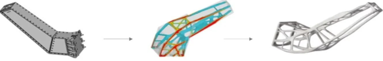
The recent advances in topological optimization and additive manufacturing yield an increasing number of complex shapes with improved tradeoff between weight and structural strength. Such shapes, common in modern design of satellites where weight reduction is crucial (Fig. 1), challenge all subsequent radiative thermal simulations as the objects contain many more free-form surface elements and obstacles.
Fig. 1. Antenna bracket. Advances in topological optimization and additive manufacturing yield increasingly complex shapes with reduced weight. Left: original design. Middle: topological optimization. Right: new design.
Simultaneously, an increasing number of computational engineering applications require real-time simu-lations, where time constraints are strict. In this context, real-time simulations applied to the aforementioned complex objects require approximate simulations which trade accuracy for time. Such approximations are commonly achieved through either thermal model reduction or geometric simplification. This paper contains instead a proposition to compute view factors progressively, with a carefully optimized tradeoff between accuracy and time.
A. State of the Art
Computing geometric view factors of complex objects is a key concern when dealing with radiosity or thermal simulation [1]. Ritoux proposed closed form formulae for canonical geometric primitives such as parallel rectangles [2]. While they provide substantial accelerations compared to nomograms, such closed forms must be recomputed for each configuration and complex objects are not always decomposable into canonical geometric
1∗ Ph.D. Student, Dorea Technology, 75 Chemin de l’Olivet, 06110 Le Cannet, FRANCE 2† CEO, Dorea Technology, 75 Chemin de l’Olivet, 06110 Le Cannet, FRANCE
primitives. Schr¨oder and Hanrahan later proposed a closed form solution for general polygon-to-polygon form factors, based on the contour integral of the form factor [3]. Closed form formulae alone do not lend to the fast and exact evaluation of obstructed form factors between complex objects, when occlusions occur due to obstacles between surface elements. More general situations require both numerical approaches to approximate geometric view factors and detecting obstacles. Numerical approximation of integrals via adaptive quadratures is an art in itself, and detecting obstacles between two surface elements, commonly performed via ray-shooting, is already a compute-intensive operation for complex objects.
Walton contributed both point-based and polygon-based adaptive quadratures, and made them available through the View3D software [4]. Jacques et al. proposed a quasi-Monte Carlo ray tracing method with improved convergence, based on the notion of isocells for point sampling [5]. D’Azevedo et al. [6] compute view factors in parallel on GPU-based computers.
Another thread of approaches proceed by geometric reduction (via mesh simplification) and thermal model reduction [7], [8]. The latter consists in reducing the system order of a partial differential system of equations, without changing its behavior significantly. The goal is to approximate the original system as accurately as possible, while reducing the order as much as possible. Gaume et al. [9] proposed a modal reduction approach, commonly used in mechanics as part of the finite element method. The principle of these methods is a change of basis for the study of structures. While these approaches are very effective, they often assume steady-state simulations. Model reduction is currently mostly performed manually, which consumes considerable effort, time and costs. This is particularly true for computing radiations as the radiative term is strongly nonlinear. Finally, finding a geometric error metric that correlates well with the notion of thermal reduction is an open problem. B. Positioning and Contributions
The focus is put on the problem of computing view factors between the facets of an object approximated by a surface triangle mesh. In particular on a progressive approach which trades accuracy for time, primarily motivated by applications where time is critical.
More specifically, a hybrid geometric/numerical method that performs an adaptive polygon-based quadrature is proposed. A hierarchical axis-aligned bounding box (AABB) tree data structure is used to accelerate obstacle detection, and a hierarchical forest data structure stores the input triangles that are recursively subdivided while the accuracy improves over time. Pairs of faces with either full or null mutual visibility are detected exactly by intersecting their 3D convex hull with the primitives of the AABB tree. These two cases lend to early terminations and closed form solutions. Faces with partial mutual visibility are adaptively subdivided using a SVM-based approach (support vector machine) such that the shadows cast by the obstacles (umbra or penumbra) are later best approximated by sums of closed form solutions. Such adaptive subdivision approach is combined with a prediction step utilizing point-based quadratures and segment shooting. This approach is validated for closed form solutions and its convergence rate is compared to state-of-the art numerical methods.
II. BACKGROUND
A uniform hemispherical heat transfer or light transport model is considered, see Fig. 2(left). The obstacles are ignored for the moment. Given two face elements 1 and 2, the (unobstructed) view factor from 1 to 2, a real number between zero and one referred to as F1→2, measures the proportion of the radiation which leaves
1 and strikes 2: F1→2= 1 A1 Z A1 Z A2 cos θ1cos θ2 π s2 dA2dA1, (1)
where A1denotes the area of 1, s2denotes the squared distance from 1 to 2, and θ1denotes the angle between
the normal vector of 1 and the segment between 1 and 2.
While such a (4D) integral can be approximated numerically via a point-based quadrature scheme, its evaluation is very compute-intensive for complex objects with many faces. In the setting where the input object is already approximated by a surface triangle mesh, using closed form polygon-to-polygon formulae between each pair of facets [3] is a viable solution.
In more general situations, each elementary term of the above integral depends on the obstacles between 1 and 2. Similarly, the obstructed view factor OF1→2 between two facets F1 and F2 ranges between 0 and
the unobstructed view factor F1→2, depending on the size and shape of the obstacles. More specifically, three
configurations can occur: (1) no visibility (OF1→2= 0) due to full occlusion generated by the obstacles, (2) full
visibility (no obstacles between the two facets, OF1→2= F1→2) and (3) partial visibility due to partial occlusion
(OF1→2= r × F1→2), where r denotes the visibility ratio. Assume that facet F1 emits light under the uniform
hemispherical model. The partial visibility case occurs when the obstacles cast shadows onto facet F2, possibly
with a complex mix between umbra and penumbra. The performance of an adaptive polygon-based quadrature relates to the capability to (1) recursively split the facets such that closed-form formulas applied to sub-facets approximate well the real view factor, and (2) compute or even predict the visibility ratio.
Fig. 2. Background elements. Left: hemispherical model. Middle left: two facets with full mutual visibility. Middle right: facets with partial visibility. Right: polygon-based quadrature. Two images taken from Walton [4].
III. PROGRESSIVEVIEWFACTORS
The approach detailed here takes as input a surface triangle mesh with F facets, where each facet is oriented so that the heat is emitted, under the uniform hemispherical model, in the half-space pointed by the facet normal. A facet transferring heat on both sides must thus be split into two facets with opposite orientations. The output is generated as a F × F matrix M, progressively refined over time, where each entry OFi→ jdenotes
the approximated obstructed view factor from facet i to facet j. The matrix is sparse when the input model has many obstructions. The main objective is to best trade accuracy for time while refining M.
Fig. 3. Half-space visibility between two faces. Left: each facet is contained in the half-space of the other facet, hence they see each others. Middle: one facet sees the other facet, but the converse is not true, hence they do not see each others. Right: none of the facet are contained in the half-space of the other facet, hence they do not see each others.
A. Polygon-based Quadrature
A polygon-based quadrature is favored over a point-based one primarily for its capability to compute view factors in closed form (see Fig. 4), in the absence of obstacles [3]. In addition, the numerical integration process is made recursive to offer progressiveness. The main degrees of freedom of such a progressive quadrature approach are (1) how to split the triangles into smaller convex polygon fragment, (2) the order in which the splitting operators are applied, and (3) the prediction method used when splitting operators are stopped for time constraints. Note however that the initial experiments using a basic edge-midpoint or longest edge recursive subdivision gave inferior convergence results than the simpler point-based recursion. Additional technical parameters are required to yield substantial improvements.
Fig. 4. Full versus partial visibility between two triangle facets. Left: full visibility: the closed form view factor formula is applied. Right: partial visibility due to the presence of an obstacle between the two facets. The closed form formula can no longer be applied, and the facets are recursively split into smaller polygons by bisection.
a) Initialization: The method is initialized by first assigning an index i to each facet of the input mesh. Then an iteration over each pair of facets ( fi, fj) is done, where i < j, to check whether facets i and j
are mutually (entirely or partially) in their visible half-space. In the negative, both OFi→ j and OFj→i are set to
b) Numerical Integration: For each pair of (root) facets ( fi, fj) the core principle of the numerical
integration approach consists in summing closed form view factors between convex polygons that correspond to the entirety or fragments of facets fi and fj. Denote by fik the kth fragment of root facet fi. When two
fragments fik and fljare fully visible 100% of their closed form view factor contribute to OFi→ j and OFj→i.
When they are partially visible both fk
i and flj are subject to further recursion via adaptive splitting. Section
III-B details the adaptive splitting procedure.
A hierarchical forest data structure is used to store the facet fragments. More specifically, the forest is a list of trees, where each tree is initialized by a facet of the input mesh. The facet fragments fik of root facet fi,
generated by recursive splitting, are stored as nodes of a tree. A leaf node has no children. Each split operator, occurring on a leaf node of a tree, generates new facet fragments (partitioning fik) stored as children of the split node. In addition, each leaf node stores a list of visible nodes that are correspond to all or fragments of other facets. See Fig. 5.
Fig. 5. Forest data structure. Top: root nodes corresponding to input triangle facets. Middle: children of root nodes. Splitting lines are depicted in red. Solid blue lines depict the list of fully visible nodes, and dashed blue lines depict the partially visible nodes. Only a subset of blue arrows are shown for clarity. Closed forms are used between pairs of fully visible nodes (grey polygons). Bottom: children of middle row. The recursive splitting occur only for partially visible nodes.
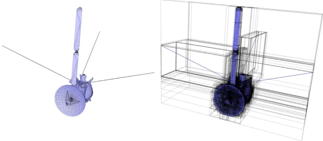
For complex input models, detecting full visibility or occlusion between pairs of convex polygons (facet fragments) requires complex geometric operations. Departing from the common segment-shooting approach which only provides approximate answers, the 3D convex hull of the polygon pair is computed exactly using an exact arithmetic kernel [10], and computes its intersection with the input triangle facets (minus the two facets containing the polygons). As this process is very compute-intensive when performed in brute force against all input facets, an accelerating, hierarchical data structure in the form of a static axis-aligned bounding box (AABB) tree is very useful [11] (see Fig. 6).
Fig. 6. AABB tree applied to Cassini 3D model. Left: input surface triangle mesh. Right: mesh and its corresponding AABB tree.
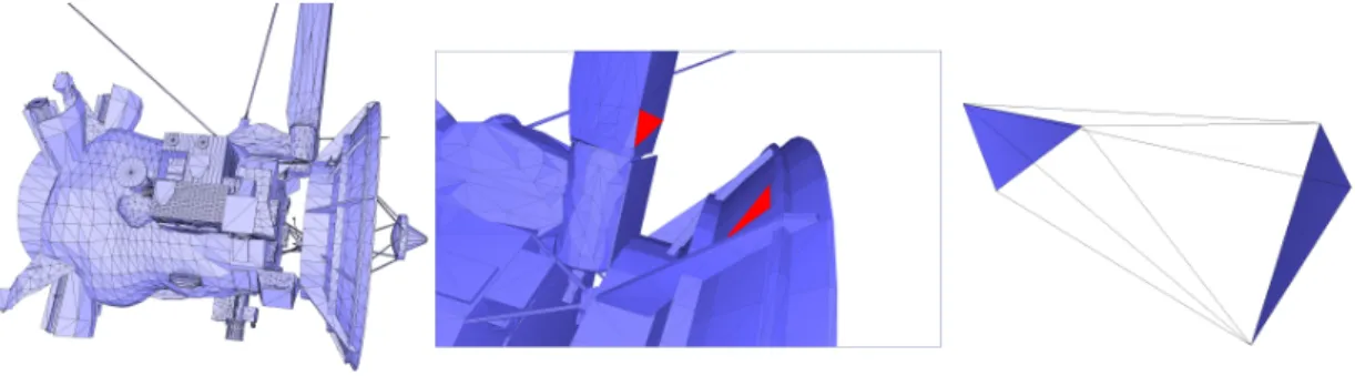
The convex hull, a convex 3D polyhedron with two facets coinciding with the two facet fragments (see Fig. 7), is tessellated into tetrahedra, and the AABB tree is tested against intersections with these tetrahedra. If
none of the input facets are intersected then the two polygon fragments are fully visible. Testing full occlusion is achieved by checking that the convex hull is disconnected by its intersection with the input facets. More specifically, disconnection is established when the source and target facet fragments are disconnected by the union of input facets intersected by the convex hull.
While computing 3D convex hulls is relevant for the full visibility/occlusion cases as they lend to early ending of the recursive splitting procedure, it is irrelevant and too expensive for pairs of facet fragments with partial mutual visibility. For this reason, a preliminary filtering phase based on line-probing is added, that throws a user-specified number of line segments and performs intersection against the input facets. More specifically, each node created in the tree is point-sampled uniformly, then random line segments connecting two samples on each fragment of the pair are queried against intersection with the AABB tree. If none of them intersect, an exact full visibility test is done. If all of them intersect, an exact full occlusion test is processed. Otherwise, the visibility is considered partial and a recursive splitting is proceeded. Section III-C details a prediction procedure that leverages the intersections with the probing line segments.
It is observed that the quality of the above point sampling is important for both effective filtering and quality prediction. Thus a bounded centroidal Voronoi diagram via Lloyd relaxation [12] is computed to generate very uniform point samples on each facet fragment of the nodes. Fig. 8 illustrates the importance of a carefully optimized point sample in terms of uniformity, by comparing the convergence rates between a simple random and an optimized uniform sample.
B. Adaptive Splitting
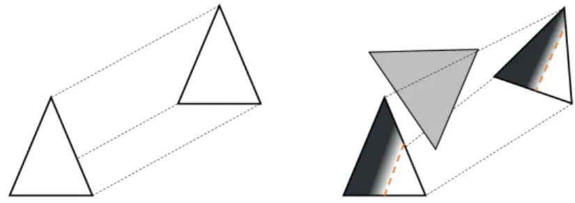
A common method for dividing triangles consists of performing longest-edge or all-edges bisection [4]. The longest edge approach favors isotropic elements while the midpoint preserves the shape of the root triangles. As isotropy and shape-preserving are both irrelevant properties to best approximate the view factors for partially visible situations, i.e. on areas with penumbra. More specifically, it would be ideal to split the input triangles into polygons whose shape adapts to the local penumbra, e.g. along the zero curvature direction in the parabolic situation. Fig. 9 illustrates a simplified setting with two canonical triangles (source and target), parallel and spaced apart from each other, with one obstacle triangle in-between, whose projection covers half of both triangles. Assume that the source emits light under the hemispherical model. The obstacles casts a shadow on the target, whose grading (transition from white to black) depends on the distance between the source and the target. Assume a dense point-sampling of the source, and line-probes randomly selected between the source and target. Probes intersecting the obstacles are depicted in red, and blue otherwise. The goal is to find the splitting line that best separates (classify) the blue from the red samples. This problem is solved via a support vector machine (SVM) approach [13] that involves solving a linear program. More specifically, the signed distance function from the samples to the splitting line is maximized. Where the confidence in the best separating line is low, i.e. when there is no privileged splitting direction, the longest edge bisection approach is adopted instead. C. Prediction
The above progressive numerical integration algorithm sums up only closed forms for pairs of facet fragments that are fully visible, and each partially visible case lends to recursive splitting into smaller fragments. The real geometric view factors are thus systematically underestimated during the course of the recursion, as if the visibility ratio mentioned in Section II is estimated to zero. One way to reduce such an underestimation is to perform a prediction of the visibility ratio for all pairs of partially visible fragments.
Fig. 7. 3D convex hull on Cassini 3D model, courtesy of nasa3d.arc.nasa.gov. Left: input surface triangle mesh. Middle: closeup on a pair of facets. Right: 3D convex hull of the facet pair.
Fig. 8. Convergence rates. Plot of the accuracy against number of quadrature points, for the uniform sampling case (left top triangle) and bounded centroidal Voronoi diagram (left bottom triangle). No prediction is used for this case.
Fig. 9. Adaptive splitting for partial visibility. Left: two canonical triangles and one obstacle in-between. Middle left: the obstacle is close to the source facet. Middle Right: the obstacle is equidistant from the source and target facets. Right: optimal splitting line.
The prediction method detailed here leverages the line probes shot for filtering out the exact full visibil-ity/occlusion tests (see above). More specifically, the ratio r between the number of probes not intersecting the obstacles and the total number of probes shot is recorded. While a trivial linear predictor y = x (i.e., r directly taken as visibility ratio) yields satisfactory results, it should take into account that r = 1, respectively r= 0 does not imply full visibility, respectively full occlusion (remind that full visibility or occlusion would have been detected earlier by the exact test). Instead an improved predictor of the visibility ratio is computed via degree-5 polynomial fitting regression (Fig. 10(left)) of ground-truth data generated offline on a series of complex models, where ground-truth data correspond to visibility ratio derived from accurate estimates of the real geometric view factors, for all possible ratios of probes intersected over shot. Fig. 10(right) plots the accuracy of view factors against the number of polygon quadrature elements, with and without prediction.
Fig. 10. Prediction. Left: predictor of the visibility ratio via degree-5 polynomial curve fitting. Right: convergence rate with and without prediction, i.e. accuracy of view factors against number of quadrature polygons, in log scale.
IV. EXPERIMENTS
The method is implemented in C++ using the following libraries: The Computational Geometry Algorithms Library (CGAL) [10], eigen [14], libsvm [13] and the random forest template library [15].
A. Validation
For numerical validation the implementation of the closed form formulation from Schr¨oder and Hanrahan [3] had to be validated with the canonical configurations of Ritoux [2]. Then the point-based and polygon-based quadratures have been tested by verifying proper convergence to the closed form in full visibility, then with View3D [4] in the presence of obstacles (Fig. 11). Such validations have been performed first for simple
configurations, mechanical parts then satellite models. Note that for View3D the means to control accuracy are either the maximum recursion depth or the convergence stopping criterion. However, it does not offer progressiveness with fine-grain as it is done in this paper, and the convergence criterion is recommended to be larger than 1.0e−6 because intermediate calculations are accurate only to single precision. Most geometric operations performed in this approach utilize the exact predicates and accurate constructions offered by the CGAL library [10].
Fig. 11. Validation with View3D. Both average and max errors of geometric view factors between all pairs of facets that are fully or partially visible are computed. Left: Average error. Right: Max error.
B. Convergence Rates
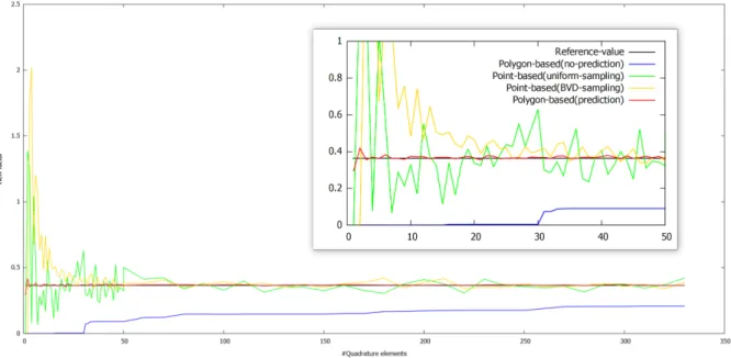
Fig. 12 illustrates the methodological advances in the course of the project. A simple polygon-based quadrature is less accurate than a point-based quadrature, even when the point sample is carefully optimized using a bounded centroidal Voronoi diagram (referred to as BVD in the caption). However, activating the prediction step offers a substantial improvement, as highlighted by the closeup. Note that these plots compare similarly when plotting accuracy against time.
Fig. 12. Convergence rates. Plot of the accuracy of view factors, with respect to reference values, against the number of quadrature elements (#points or #polygon fragments elements per area unit), be they points or polygons. The closeup on the right depicts the curves between 0 and 50 quadrature elements.
V. CONCLUSION
In this paper, a progressive approach for computing geometric view factors between facets of surface triangle meshes has been proposed. The numerical integration approach proceeds by recursive polygon-based quadrature, coupled with adaptive facet splitting, line probing and closed form formulae for fully visible configurations, and prediction for partially visible configurations.
A special care has been put at numerical precisions and exactness of early termination tests such as detection of full visibility or occlusions. The prediction step yields substantial improvements of convergence rates. One limitation of this approach is that linear elements are taken as input. Curved models thus require a preliminary meshing step which introduces an approximation error. Another limitation comes from the limited progressiveness for low accuracy: the initial output matrix of view factors still requires a quadratic number of operations in the number of facets of the input mesh. It would be interesting to explore an approach using e.g. recursive facet clustering coupled with far field approximation in order to generate a coarser output matrix in shorter times.
As future work the approach detailed in this paper can be adapted to curved, higher-order elements such as B´ezier or NURBS surfaces. This would require devising closed form formulae for these elements and approximation algorithms [16]. Beyond leveraging the line probes for prediction, another promising direction consists of (1) exploiting the information collected during the descent in the tree during recursion, and (2) computing descriptors of the obstacles intersected by the probes, and leveraging modern machine learning methods for performing a more accurate regression of the visibility ratio. More specifically, the nodes of the tree can record the probe ratios for their partially visible nodes, such that it is possible to regress over not just the current probe ratio, but also its ancestors in the tree. In addition, the AABB tree not only computes intersection tests, but can also return the list of facets intersected. Some geometric descriptors are computed for these facets (areas, aspect ratios, spread between source and target fragments, project area in bisector plane during source and target, etc.), including statistics over these quantities (average, variance), and given to a random forest regression method [15]. However, it should be kept in mind that computing the descriptors may be compute-intensive, and may thus impact the convergence rates.
REFERENCES
[1] H. C. Hottel and A. F. Sarofim, Radiation transfer (Mc Graw-Hill). Mc Graw-Hill, 1967. [2] G. Ritoux, “Evaluation num´erique des facteurs de forme,” 1982.
[3] P. Schroeder and P. Hanrahan, “A Closed Form Expression for the Form Factor between Two Polygons,” 1993. [4] G. Walton, “Calculation of Obstructed View Factors by Adaptive Integration,” Tech. Rep. 6925, NIST, 2002.
[5] L. Jacques, L. Masset, and G. Kerschen, “Ray Tracing Enhancement For Space Thermal Analysis: Isocell Method,” 2013. [6] E. DAzevedo, Z. Hu, S.-Q. Su, and K. Wong, “Solving a large scale radiosity problem on GPU-based parallel computers,” 2014. [7] M. Deiml, M. Suderland, P. Reiss, and M. Czupalla, “Development and evaluation of thermal model reduction algorithms for
spacecraft,” 2015.
[8] G. Fernndez-Rico, I. Prez-Grande, A. Sanz-Andres, I. Torralbo, and J. Woch, “Quasi-autonomous thermal model reduction for steady-state problems in space systems,” 2016.
[9] B. Gaume, F. Joly, and O. Qumner, “Modal reduction for a problem of heat transfer with radiation in an enclosure,” International Journal of Heat and Mass Transfer, vol. 141, pp. 779 – 788, 2019.
[10] The CGAL Project, CGAL User and Reference Manual. CGAL Editorial Board, 5.0.1 ed., 2020.
[11] P. Alliez, S. Tayeb, and W. C., “3D fast intersection and distance computation,” in CGAL User and Reference Manual, CGAL Editorial Board, 5.0.1 ed., 2020.
[12] J. Tournois, P. Alliez, and O. Devillers, “2D Centroidal Voronoi Tessellations with Constraints,” Numerical Mathematics: Theory, Methods and Applications, vol. 3, no. 2, pp. 212–222, 2010.
[13] C. Chang and C. Lin, “LIBSVM: A library for support vector machines,” ACM Transactions on Intelligent Systems and Technology, vol. 2, pp. 27:1–27:27, 2011.
[14] G. Guennebaud, B. Jacob, et al., “Eigen v3.” http://eigen.tuxfamily.org, 2010. [15] S. Walk, “Random Forest Template Library,” 2019.
[16] L. Feng, P. Alliez, L. Bus´e, H. Delingette, and M. Desbrun, “Curved Optimal Delaunay Triangulation,” ACM Transactions on Graphics, vol. 37, no. 4, p. 16, 2018.