arXiv:1210.4257v2 [astro-ph.EP] 25 Feb 2013
Astronomy & Astrophysicsmanuscript no. aa˙2012˙20561 ESO 2013c
February 26, 2013
WASP-64 b and WASP-72 b: two new transiting highly irradiated
giant planets
⋆
M. Gillon
1, D. R. Anderson
2, A. Collier-Cameron
3, A. P. Doyle
2, A. Fumel
1, C. Hellier
2, E. Jehin
1, M. Lendl
4,
P. F. L. Maxted
2, J. Montalb´an
1, F. Pepe
4, D. Pollacco
5, D. Queloz
4, D. S´egransan
4, A. M. S. Smith
2, B. Smalley
2,
J. Southworth
2, A. H. M. J. Triaud
4, S. Udry
4, R. G. West
61Institut d’Astrophysique et de G´eophysique, Universit´e de Li`ege, All´ee du 6 aoˆut 17, Sart Tilman, Li`ege 1, Belgium 2Astrophysics Group, Keele University, Staffordshire, ST5 5BG, United Kingdom
3School of Physics and Astronomy, University of St. Andrews, North Haugh, Fife, KY16 9SS, UK 4Observatoire de Gen`eve, Universit´e de Gen`eve, 51 Chemin des Maillettes, 1290 Sauverny, Switzerland 5Department of Physics, University of Warwick, Coventry CV4 7AL, UK
6Department of Physics and Astronomy, University of Leicester, Leicester, LE1 7RH, UK
Received date / accepted date
ABSTRACT
We report the discovery by the WASP transit survey of two new highly irradiated giant planets. WASP-64 b is slightly more massive (1.271 ± 0.068 MJup) and larger (1.271 ± 0.039 RJup) than Jupiter, and is in very-short (a = 0.02648 ± 0.00024 AU, P = 1.5732918 ±
0.0000015 days) circular orbit around a V=12.3 G7-type dwarf (1.004 ± 0.028 M⊙, 1.058 ± 0.025 R⊙, Teff= 5500 ± 150 K). Its size
is typical of hot Jupiters with similar masses. WASP-72 b has also a mass a bit higher than Jupiter’s (1.461+0.059
−0.056 MJup) and orbits
very close (0.03708 ± 0.00050 AU, P = 2.2167421 ± 0.0000081 days) to a bright (V=9.6) and moderately evolved F7-type star (1.386 ± 0.055 M⊙, 1.98 ± 0.24 R⊙, Teff= 6250 ± 100 K). Despite its extreme irradiation (∼ 5.5 × 10⁹erg s−1cm−2), WASP-72 b has a
moderate size (1.27 ± 0.20 RJup) that could suggest a significant enrichment in heavy elements. Nevertheless, the errors on its physical
parameters are still too high to draw any strong inference on its internal structure or its possible peculiarity.
Key words.stars: planetary systems - star: individual: WASP-64 - star: individual: WASP-72 - techniques: photometric - techniques: radial velocities - techniques: spectroscopic
1. Introduction
The booming study of exoplanets allow us to assess the diver-sity of the planetary systems of the Milky Way and to put our own solar system in perspective. Notably, ground-based transit surveys targeting relatively bright (V < 13) stars are detecting at an increasing rate short-period giant planets amenable for a thorough characterization (orbit, structure, atmosphere), thanks to the brightness of their host star, the favorable planet-star size ratio and their high stellar irradiation (e.g. Winn 2010). With its very high detection efficiency, the WASP transit survey (Pollacco et al. 2006) is one of the most productive projects in that domain. In this context, we report here the detection by WASP of two new giant planets, WASP-64 b and WASP-72 b, transiting relatively bright Southern stars. Section 2 presents the WASP discovery photometry, and high-precision follow-up observa-tions obtained from La Silla ESO Observatory (Chile) by the TRAPPIST and Euler telescopes to confirm the transits and planetary nature of both objects and to determine precisely the systems parameters. In Sect. 3, we present the spectroscopic de-termination of the stellar properties and the derivation of the sys-tems parameters through a combined analysis of the follow-up
Send offprint requests to: [email protected]
⋆ The photometric time-series used in this work are only available
in electronic form at the CDS via anonymous ftp to cdsarc.u-strasbg.fr (130.79.128.5) or via http://cdsweb.u-strasbg.fr/cgi-bin/qcat?J/A+A/
photometric and spectroscopic time-series. Finally, we discuss our results in Sect. 4.
2. Observations
2.1. WASP transit detection photometry
The stars 1SWASPJ064427.63-325130.4 (WASP-64; V=12.3,
K=11.0) and 1SWASPJ024409.60-301008.5 (WASP-72;
V=10.1, K=9.6) were observed by the Southern station of
the WASP survey (Hellier et al. 2011) between 2006 Oct 11 and 2010 Mar 12 and between 2006 Aug 11 and 2007 Dec 31, respectively. The 17981 and 6500 pipeline-processed photometric measurements were detrended and searched for transits using the methods described by Collier-Cameron et al. (2006). The selection process (Collier-Cameron et al. 2007) identified WASP-72 as a high priority candidate showing periodic low-amplitude (2-3 mmag) transit-like signatures with period of 2.217 days. For WASP-64, similar transit-like signals with a period of 1.573 days were also detected, not only on the target itself but also on a brighter star at 28”, 1SWASPJ064429.53–325129.5 (TYC7091-1288-1, V=12.3,
K=11.0). Fig. 1 presents for TYC7091-1288-1 and WASP-64
the WASP photometry folded on the deduced transit ephemeris. Fig. 2 does the same for WASP-72.
A search for periodic modulation was applied to the photom-etry of WASP-72, using for this purpose the method described in Maxted et al. (2011). No periodic signal was found down
to the mmag amplitude. We did not perform such a search for TYC7091-1288-1 and WASP-64, as these two stars are blended together at the spatial resolution of the WASP instrument (see below). Still, a Lomb-Scargle periodogram analysis of their pho-tometric time-series did not reveal any significant power excess.
2.2. Follow-up photometry 2.2.1. WASP-64
WASP-64 is at 28” West from TYC7091-1288-1, close enough to have most of its point-spread function (PSF) enclosed in the smallest of the WASP photometry extraction apertures (ra-dius=34”, see Fig. 3). Both objects have an entry in the WASP database, because it is based on an input catalogue of star po-sitions. Still, the WASP light curve obtained with an aperture centered on WASP-64 is of poorer quality (see Fig. 1), because the centering algorithm does not work optimally when there is a bright object off-centre in the aperture or just outside of it, while significant levels of red noise are brought by PSF variations. This explains why the transit was first detected from the photometry centered on TYC7091-1288-1. Having both stars nearly totally enclosed in the smallest apertures for both centerings prevented us to decide from the WASP photometry alone if the eclipse sig-nal detected by WASP was originating from one or the other star, so our first follow-up action was to measure on 2011 Jan 20 a transit at a better spatial resolution with the robotic 60cm tele-scope TRAPPIST (TRAnsiting Planets and PlanetesImals Small
Telescope; Gillon et al. 2011, Jehin et al. 2011) located at ESO
La Silla Observatory in the Atacama Desert, Chile. TRAPPIST is equipped with a thermoelectrically-cooled 2K × 2K CCD hav-ing a pixel scale of 0.65” that translates into a 22’ × 22’ field of view. Differential photometry was obtained with TRAPPIST for both stars on the night of 2011 Jan 20, corresponding to a transit window as derived from WASP data. These observations were obtained with the telescope focused and through a special ‘I + z’ filter that has a transmittance >90% from 750 nm to beyond 1100 nm1. The positions of the stars on the chip were maintained to within a few pixels over the course of the run, thanks to a ‘soft-ware guiding’ system deriving regularly an astrometric solution for the most recently acquired image and sending pointing cor-rections to the mount if needed. After a standard pre-reduction (bias, dark, flatfield correction), the stellar fluxes were extracted from the images using the IRAF/DAOPHOT2aperture photometry
software (Stetson, 1987). Several sets of reduction parameters were tested, and we kept the one giving the most precise pho-tometry for the stars of similar brightness as the target. After a careful selection of a set of 22 reference stars, differential pho-tometry was then obtained. This reduction procedure was also applied for the subsequent TRAPPIST runs.
This first TRAPPIST run resulted in a flat light curve for TYC7091-1288-1, while the light curve for WASP-64 showed a clear transit-like structure (Fig. 3), identifying thus WASP-64 as the source of the transit signal. A second (partial) transit was observed in the I + z filter on 2011 Feb 22 to better constrain the shape of the eclipse (Fig. 4, second light curve from the top). As for the following WASP-64 transits, the telescope was defo-cused to ∼3” to improve the duty cycle and average the pixel-to-pixel effects. A global analysis of the two first TRAPPIST
1 http://www.astrodon.com/products/filters/near-infrared/
2 IRAF is distributed by the National Optical Astronomy Observatory, which is operated by the Association of Universities for Research in Astronomy, Inc., under cooperative agreement with the National Science Foundation.
transit light curves led to an eclipse depth and shape compatible with the transit of a giant planet in front of a solar-type star. Our next action was to observe a third transit with TRAPPIST, this time in the V filter to assess the chromaticity of the transit depth (Fig. 4, third light curve from the top). The analysis of the re-sulting light curve led to a transit depth consistent with the one measured in the I +z filter, as expected for a transiting planet. We then observed an occultation window in the z′-band on 2011 Apr
30. We could not detect any eclipse in the resulting photometric time-series (Fig. 5), which was again consistent with the tran-siting planet scenario. At this stage, we began our spectroscopic follow-up of WASP-64 that confirmed the solar-type nature of WASP-64 and the planetary nature of its eclipsing companion (see Sec. 2.3).
Once the planetary nature of WASP-64 b was confirmed, we observed seven more of its transits with TRAPPIST, using then a blue-blocking filter3that has a transmittance >90% from 500 nm to beyond 1000 nm. The goal of using this very wide red filter is to maximize the signal-to-noise ratio (S/N) while minimizing the influence of moonlight pollution, differential extinction and stellar limb-darkening on the transit light curves. The resulting light curves are shown in Fig. 4. The transit of 2011 Oct 19 was also observed in the Gunn-r filter with the EulerCam CCD cam-era at the 1.2-m Euler Telescope at La Silla Observatory. This nitrogen-cooled camera has a 4k × 4k E2V CCD with a 15’ × 15’ field of view (scale=0.23”/pixel). Here too, a defocus was ap-plied to the telescope to optimize the observation efficiency and minimize pixel-to-pixel effects, while flat-field effects were fur-ther reduced by keeping the stars on the same pixels, thanks to a ‘software guiding’ system similar to the one of TRAPPIST (Lendl et al. 2012). The reduction was similar to that performed on TRAPPIST data. The resulting light curve is also shown in Fig. 4.
2.2.2. WASP-72
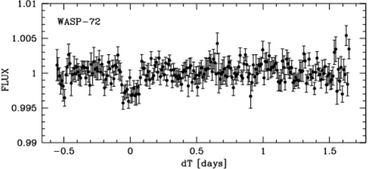
We monitored for WASP-72 five transits with TRAPPIST (see Table 1 and Fig. 6), two partial and two full transits in the I + z filter and one full transit in the blue-blocking filter. For the three transits observed in 2011, the telescope was defocused to ∼3”. A first partial transit was observed in 2011 Jan 21 in the I + z filter at high airmass, confirming the low-amplitude eclipse detected by WASP (Fig. 6, first light curve from the top). The next season, a full transit was observed on 2011 Oct 25 in the blue-blocking filter. A technical problem damaged these data: a shutter problem led to a scatter twice higher than expected. In 2011, a partial transit was also observed in the I + z filter on Dec 4. In 2012, two new full transits were observed with TRAPPIST in the I + z filter. For these two last runs, the telescope was kept focused to minimize the effects of a focus drift problem with an amplitude stronger for out-of-focus observations. We are still investigating the origin of this technical problem. Two transits of WASP-72 were also observed with Euler on 2011 Nov 26 and 2012 Nov 16, with the same strategy than for WASP-64. For the second Euler transit, a crash of the tracking system led to significant shifts of the stars on the detectors (up to 50 pixels), giving rise to significant systematic effects in the differential photometry (see Fig. 6)
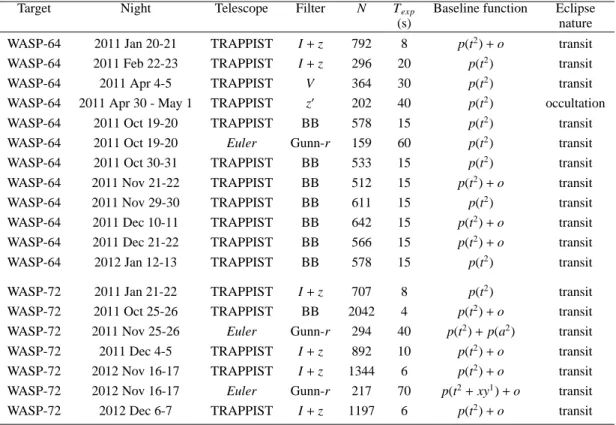
Table 1 presents a summary of the follow-up photometric time-series obtained for WASP-64 and WASP-72.
Fig. 3. 280”×280” TRAPPIST I + z image centered on TYC7091-1288-1. North is up and East is left. The three concentric circles
indicate the three photometry extraction apertures used in the WASP pipeline. WASP-64 is the closest star to the right of TYC7091-1288-1. For both stars, the light curve obtained by TRAPPIST on 2011 Jan 20 is shown (cyan=unbinned, black=binned per intervals of 0.005d).
Target Night Telescope Filter N Texp Baseline function Eclipse
(s) nature
WASP-64 2011 Jan 20-21 TRAPPIST I + z 792 8 p(t2) + o transit WASP-64 2011 Feb 22-23 TRAPPIST I + z 296 20 p(t2) transit
WASP-64 2011 Apr 4-5 TRAPPIST V 364 30 p(t2) transit
WASP-64 2011 Apr 30 - May 1 TRAPPIST z′ 202 40 p(t2) occultation
WASP-64 2011 Oct 19-20 TRAPPIST BB 578 15 p(t2) transit
WASP-64 2011 Oct 19-20 Euler Gunn-r 159 60 p(t2) transit
WASP-64 2011 Oct 30-31 TRAPPIST BB 533 15 p(t2) transit
WASP-64 2011 Nov 21-22 TRAPPIST BB 512 15 p(t2) + o transit
WASP-64 2011 Nov 29-30 TRAPPIST BB 611 15 p(t2) transit
WASP-64 2011 Dec 10-11 TRAPPIST BB 642 15 p(t2) + o transit WASP-64 2011 Dec 21-22 TRAPPIST BB 566 15 p(t2) + o transit
WASP-64 2012 Jan 12-13 TRAPPIST BB 578 15 p(t2) transit
WASP-72 2011 Jan 21-22 TRAPPIST I + z 707 8 p(t2) transit
WASP-72 2011 Oct 25-26 TRAPPIST BB 2042 4 p(t2) + o transit WASP-72 2011 Nov 25-26 Euler Gunn-r 294 40 p(t2) + p(a2) transit WASP-72 2011 Dec 4-5 TRAPPIST I + z 892 10 p(t2) + o transit WASP-72 2012 Nov 16-17 TRAPPIST I + z 1344 6 p(t2) + o transit WASP-72 2012 Nov 16-17 Euler Gunn-r 217 70 p(t2+ xy1) + o transit WASP-72 2012 Dec 6-7 TRAPPIST I + z 1197 6 p(t2) + o transit
Table 1. Summary of follow-up photometry obtained for WASP-64 and WASP-72. N= number of measurements. Texp= exposure
time. BB = blue-blocking filter. The baseline functions are the analytical functions used to model the photometric baseline of each light curve (see Sec. 3.2). p(t2) denotes a quadratic time polynomial, p(a2) a quadratic airmass polynomial, p(xy1) a linear function
of the stellar position on the detector, and o an offset fixed at the time of the meridian flip.
2.3. Spectroscopy and radial velocities
Once WASP-64 and WASP-72 were identified as high priority candidates, we gathered spectroscopic measurements with the
CORALIEspectrograph mounted on Euler to confirm the plan-etary nature of the eclipsing bodies and obtain mass measure-ments. 16 usable spectra were obtained for WASP-64 from 2011 May 2 to 2011 November 7 with an exposure time of 30 minutes. For WASP-72, 18 spectra were gathered from 2011 January 9 to 2011 December 29, here too with an exposure time of 30
min-utes. For both stars, radial velocities (RVs) were computed by weighted cross-correlation (Baranne et al. 1996) with a numer-ical G2-spectral template giving close to optimal precisions for late-F to early-K dwarfs, from our experience. The resulting RVs are shown in Table 2.
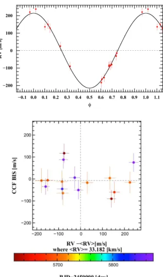
The RV time-series show variations that are consistent with planetary-mass companions. Preliminary orbital analyses of the RVs resulted in periods and phases in excellent agreement with those deduced from the WASP transit detections (Fig. 7 & 8,
Fig. 1. WASP photometry for TYC7091-1288-1 (top) and
WASP-64 (bottom) folded on the best-fitting transit ephemeris from the transit search algorithm presented in Collier Cameron et al. (2006), and binned per 0.01d intervals.
Fig. 2. WASP photometry for WASP-72 folded on the
best-fitting transit ephemeris from the transit search algorithm pre-sented in Collier Cameron et al. (2006), and binned per 0.01d intervals.
upper panels). For WASP-64, assuming a stellar mass M∗ =
0.98 ± 0.09 M⊙ (Sect. 3.1), the fitted semi-amplitude K = 212 ± 17 m s−1translates into a secondary mass slightly higher
than Jupiter’s, Mp = 1.19 ± 0.12 MJup. The resulting orbital
ec-centricity is consistent with zero, e = 0.05+0.06
−0.03. For WASP-72,
assuming a stellar mass M∗ = 1.23 ± 0.10 M⊙ (Sect. 3.1), the fitted semi-amplitude K = 179 ± 6 m s−1translates into a
sec-ondary mass Mp = 1.31 ± 0.08 MJup, while the deduced orbital
eccentricity is also consistent with zero, e = 0.05+0.03 −0.03.
A model with a slope is slightly favored in the case of WASP-72, its value being -82 ± 22 m s−1 per year. Indeed, the
re-spective values for the Bayesian Information Criterion (BIC; Schwarz 1978) led to likelihood ratios (Bayes factors) between 10 and 55 in favor of the slope model, depending if the orbit was assumed to be circular or not. Such values for the Bayes factor
-0.05
0
0.05
1
1.1
1.2
1.3
1.4
dT [days]
Fig. 4. Follow-up transit photometry for WASP-64 b. For each
light curve, the best-fit transit+baseline model deduced from the global analysis is superimposed (see Sec. 3.2). The light curves are shifted along the y-axis for clarity. BB = Blue-blocking filter.
are not high enough to be decisive, and more RVs will be needed to confirm this possible trend.
To confirm that the RV signal originates well from planet-mass objects orbiting the stars, we analyzed the CORALIE cross-correlation functions (CCF) using the line-bisector technique de-scribed in Queloz et al (2001). The bisector spans revealed to be stable, their standard deviation being close to their average error (57 vs 47 m s−1for WASP-64 and 28 vs 24 m s−1for WASP-72). No evidence for a correlation between the RVs and the bisec-tor spans was found (Fig. 7 & 8, lower panels), the slopes
de-Fig. 5. TRAPPIST z′time-series photometry obtained during an
occultation window of WASP-64 b, unbinned and binned per in-tervals of 0.005d. An occultation model assuming a circular orbit and a depth of 0.5% is superimposed for comparison.
duced from linear regression being −0.02 ± 0.08 (WASP-64) and
−0.01 ± 0.04 (WASP-72). These values and errors makes any
blend scenario very unlikely. Indeed, if the orbital signal of a putative blended eclipsing binary (EB) is able to create a clear periodic wobble of the sum of both CCFs, it should also create a significant periodic distortion of its shape, resulting in corre-lated variations of RVs and bisector spans having the same order of magnitude (Torres et al. 2004). The power of this effect to identify blended EBs among transit candidates was first demon-strated by the classical case of CSC 01944-02289 (Mandushev et al. 2005), for which the bisector spans varied in phase with the RVs and with an amplitude about twice lower. Another famous case is the HD 41004 system (Santos et al. 2002), with a K-dwarf blended with a M-dwarf companion (separation ∼0.5”) which is itself orbited by a short-period brown dwarf. For this extreme system, the RVs show a clear signal at the period of the brown dwarf orbit (1.3 days) and with an amplitude ∼ 50 m s−1that
could be taken for the signal of a sub-Saturn mass planet orbit-ing the K-dwarf, except that the slope of the bisector-RV relation is 0.67±0.03, clearly revealing that the main spectral component of the CCF is not responsible for the observed signal. In the case of WASP-64 and 72, the 3-σ upper limits of 0.23 and 0.09 that we derived from Monte-Carlo simulations for the bisector-RV slopes combined with the much higher amplitude of the mea-sured RV signals allow us to confidently infer that the RV signal is actually originating from the target stars. This conclusion is strengthened by the consistency of the solutions derived from the global analysis of our spectroscopic and photometric data (see next Section). We conclude thus that the stars WASP-64 and WASP-72 are transited by a giant planet every ∼1.573 and
∼2.217 days, respectively. Of course, we cannot exclude that the
light of those stars is not diluted by a well-aligned object able to bias our inferences about the planets. Still, our multicolor transit photometry showing no dependance of the transit depths on the wavelength, and the absence of any detectable second spectra in the CORALIE data strongly disfavors any significant pollution of the light of the host stars.
3. Analysis
3.1. Spectroscopic analysis - stellar properties
The CORALIE spectra of WASP-64 and WASP-72 were co-added to produce single spectra with average S/N of 60 and 80, respec-tively. The standard pipeline reduction products were used in the analysis.
-0.2
-0.1
0
0.1
0.2
0.9
1
1.1
dT [days]
Fig. 6. Follow-up transit photometry for WASP-72 b. For each
light curve, the best-fit transit+baseline model deduced from the global analysis is superimposed (see Sec. 3.2). The light curves are shifted along the y-axis for clarity.
The spectral analysis was performed using the methods given by Gillon et al. (2009a). The Hαline was used to determine
the effective temperature (Teff). For WASP-64, the Na i D and
Mg i b lines were used as surface gravity (log g) diagnostics. For WASP-72, getting an measurement of log g was more critical, as the transit photometry does not constrain strongly the stellar density (see Sec. 3.2), so we used the improved method recently described by Doyle et al. (2013) and based on the ionization balance of selected Fe i/Fe ii lines in addition to the pressure-broadened Ca i lines at 6162Å and 6439Å (Bruntt et al. 2010a),
Fig. 7. T op: CORALIE RVs for WASP-64 phase-folded on the
best-fit orbital period, and with the best-fit Keplerian model over-imposed. Bottom: correlation diagram CCF bisector spans
vs RV. The colors indicate the measurement timings.
along with the Na i D lines. The parameters obtained from the analysis are listed in Table 3. The elemental abundances were de-termined from equivalent width measurements of several clean and unblended lines. A value for microturbulence (ξt) was
deter-mined from Fe i lines using the method of Magain (1984). The quoted error estimates include those given by the uncertainties in Teff, log g and ξt, as well as the scatter due to measurement
and atomic data uncertainties.
The projected stellar rotation velocities (v sin i∗) were de-termined by fitting the profiles of several unblended Fe i lines. Values for macroturbulence (vmac) of 1.8 ± 0.3 and 4.0 ± 0.3
km s−1 were assumed for WASP-64 and WASP-72, respectively,
based on the calibration by Bruntt at al. (2010b). An instrumen-tal FWHM of 0.11 ± 0.01 Å was determined for both stars from the telluric lines around 6300Å. Best-fitting values of v sin i∗ =
3.4 ± 0.8 km s−1 (WASP-64) and v sin i
∗ = 6.0 ± 0.7 km s−1
(WASP-72) were obtained.
There is no significant detection of lithium in the spectra, with equivalent width upper limits of 2mÅ for both stars, corre-sponding to abundance upper limits of log A(Li) < 0.61 ± 0.15 (WASP-64) and log A(Li) < 1.21 ± 0.17 (WASP-72). These im-ply ages of at least a few Gyr (Sestito & Randich, 2005).
Fig. 8. T op: CORALIE RVs for WASP-72 phase-folded on the
best-fit orbital period, and with the best-fit Keplerian model over-imposed. Bottom: correlation diagram CCF bisector spans
vs RV. The colors indicate the measurement timings.
The rotation rate for WASP-64 (Prot = 15.3 ± 4.7 d) and
WASP-72 (Prot= 14.5 ± 3.1 d) implied by the v sin i∗ give
gy-rochronological ages of ∼1.2+1.2−0.7Gyr (WASP-64) and ∼ 3.7+4.0−1.9 Gyr (WASP-72) under the Barnes (2007) relation.
We obtained with CORALIE two spectra of TYC7091-1288-1, the brighter star lying at 28” East from WASP-64 (Sec. 2.2.TYC7091-1288-1, Fig. 3). The co-added spectrum has a S/N of only ∼30. A spectral analysis led to Teff∼5700K and log g ∼4.5, with no sign of any
significant lithium absorption, and a low v sin i∗ ∼4 km s−1. The
RV is ∼35 km s−1, compared to 33.2 km s−1 for WASP-64. The
cross-correlation function reveals that TYC 7091-1288-1 is an SB2 system (Fig. 8). The PPMXL catalogue (Roeser et al. 2010) shows that proper motions of both stars are consistent to within their quoted uncertainties. If these stars are physically associate, as suggested by their similar proper motions and radial veloci-ties, their angular separation corresponds to a projected distance of 9800 ± 2500 AU, which is possible for a very wide triple sys-tem. Of course, the spectra of TYC7091-1288-1 and WASP-64 are totally separated at the spatial resolution of CORALIE (typical seeing ∼1”, fiber diameter of 2”), considering the 28” separation between both objects.
Target H JDT DB-2450000 RV σRV BS (km s−1) (m s−1) (km s−1) WASP-64 5622.652685 33.1075 21.5 0.1171 WASP-64 5629.582507 33.3234 19.8 –0.0900 WASP-64 5681.541466 33.3368 23.9 –0.0601 WASP-64 5696.488635 33.0326 24.3 –0.0057 WASP-64 5706.460152 33.4079 24.3 –0.0156 WASP-64 5707.460947 33.0038 28.0 –0.0075 WASP-64 5708.461813 33.2129 25.1 –0.0169 WASP-64 5711.463695 33.3160 26.3 0.0040 WASP-64 5715.458133 33.1019 27.2 –0.0645 WASP-64 5716.463634 33.0977 26.1 –0.0121 WASP-64 5842.867334 33.0986 24.0 –0.0453 WASP-64 5861.847564 33.1559 25.4 0.0061 WASP-64 5864.795499 33.0230 18.1 –0.0346 WASP-64 5869.724123 33.1725 20.6 –0.0504 WASP-64 5871.734734 33.4248 21.1 0.0752 WASP-64 5872.762875 33.1044 20.1 0.0877 WASP-72 5570.618144 35.7945 13.3 0.0176 WASP-72 5828.890931 36.0233 11.3 0.0566 WASP-72 5829.865219 35.8029 9.8 0.0466 WASP-72 5830.866138 35.9320 11.5 0.0623 WASP-72 5832.894502 35.8391 14.6 0.0396 WASP-72 5852.780149 35.7640 15.5 0.0092 WASP-72 5856.757447 35.7288 11.5 0.0390 WASP-72 5858.689011 35.8146 15.2 –0.0198 WASP-72 5863.800340 35.7664 10.4 0.0462 WASP-72 5864.750293 36.0695 10.0 0.0292 WASP-72 5865.812141 35.7283 11.9 0.0968 WASP-72 5866.605265 36.0331 10.6 0.0734 WASP-72 5867.628720 35.7586 10.3 0.0605 WASP-72 5868.759336 35.9966 10.4 –0.0019 WASP-72 5873.808914 35.9928 10.9 0.0368 WASP-72 5886.748911 36.0460 16.3 0.0624 WASP-72 5914.700813 35.7261 9.5 0.0504 WASP-72 5924.584434 36.0624 10.0 0.0562
Table 2. CORALIE radial-velocity measurements for WASP-64
and WASP-72 (BS = bisector spans).
3.2. Global analysis
For both systems, we performed a global analysis of the follow-up photometry and the CORALIE RV measurements. The analysis was performed using the adaptive Markov Chain Monte-Carlo (MCMC) algorithm described by Gillon et al. (2012, and refer-ences therein). To summarize, we simultaneously fitted the data, using for the photometry the transit model of Mandel & Agol (2002) multiplied by a baseline model consisting of a different second-order polynomial in time for each of the light curves. We motivate the choice of this ‘minimal’ baseline model by its better ability to represent properly any smooth variation due to a com-bination of differential extinction and low-frequency stellar vari-ability, compared to other possible simple functions (scalar, lin-ear function of time or airmass). We outline that using a simple scalar as baseline model relies on the strong assumptions that the
Parameter WASP-64 WASP-72
RA (J2000) 06 44 27.61 02 44 09.60 DEC (J2000) -32 51 30.25 -30 10 08.5 V 12.29 10.88 K 10.98 9.62 Teff 5550 ± 150 K 6250 ± 100 K log g 4.4 ± 0.15 4.08 ± 0.13 ξt 0.9 ± 0.1 km s−1 1.6 ± 0.1 km s−1 v sin i∗ 3.4 ± 0.8 km s−1 6.0 ± 0.7 km s−1 [Fe/H] −0.08 ± 0.11 −0.06 ± 0.09 [Na/H] 0.14 ± 0.08 −0.03 ± 0.04 [Mg/H] 0.12 ± 0.12 [Al/H] 0.00 ± 0.08 [Si/H] 0.10 ± 0.10 0.02 ± 0.07 [Ca/H] 0.05 ± 0.16 0.07 ± 0.14 [Sc/H] 0.07 ± 0.10 0.14 ± 0.07 [Ti/H] −0.02 ± 0.11 0.07 ± 0.11 [V/H] 0.03 ± 0.16 −0.01 ± 0.08 [Cr/H] 0.01 ± 0.08 0.02 ± 0.10 [Mn/H] 0.09 ± 0.10 −0.11 ± 0.06 [Co/H] 0.06 ± 0.09 −0.06 ± 0.18 [Ni/H] −0.04 ± 0.11 −0.04 ± 0.06 log A(Li) <0.61 ± 0.15 <1.21 ± 0.17 Mass 0.98 ± 0.09 M⊙ 1.31 ± 0.11M⊙ Radius 1.03 ± 0.20 R⊙ 1.72 ± 0.31R⊙ Sp. Type G7 F7 Distance 350 ± 90 pc 340 ± 60 pc
Table 3. Basic and spectroscopic parameters of WASP-64 and
WASP-72 from spectroscopic analysis.
Notes: The values for the stellar mass, radius and surface gravity
are given here for information purpose only. The values that we finally adopted for these parameters are the ones derived from the global analysis of our data (Sec. 3.2) and are presented in Table 5 and 6. Mass and radius estimate using the calibration of Torres et al. (2010). Spectral type estimated from Teff using the
table in Gray (2008).
ensemble of comparison stars used to derive the differential pho-tometry has exactly the same color than the target, that the target is perfectly stable, and that no low-frequency noise could have modified the transit shape. For eight TRAPPIST light curves (see Table 1), a normalization offset was also part of the model to represent the effect of the meridian flip. TRAPPIST’s mount is a german equatorial type, which means that the telescope has to undergo a 180◦rotation when the meridian is reached, resulting
in different locations of the stellar images on the detector before and after the flip, and thus in a possible jump of the differential flux at the time of the flip. For the first WASP-72 Euler transit, a quadratic function of airmass had to be added to the minimal baseline model to account for the strong extinction effect caused by the high airmass (>2.5) at the end of the run. For the second WASP-72 transit observed by Euler, a normalization offset and a linear term in x- and y-position were added to model the ef-fects on the photometry of the telescope tracking problem. On their side, the RVs were represented by a classical model assum-ing Keplerian orbits (e.g. Murray & Correia 2010, eq. 65), plus a linear trend for WASP-72 (see Sec. 2.3).
The jump parameters4 in our MCMC analysis were: the planet/star area ratio (Rp/R∗)2, the transit width (from first to
last contact) W, the parameter b′ = a cos ip/R
∗ (which is the
transit impact parameter in case of a circular orbit) where a is
4 Jump parameters are the parameters that are randomly perturbed at each step of the MCMC.
Fig. 9. The cross-correlation functions for the two CORALIE
spectra of TYC7091-1288-1. Their clear asymmetry indicates the SB2 nature of the star.
the planet’s semi-major axis and ip its orbital inclination, the orbital period P and time of minimum light T0, the parameter
K2 = K
√
1 − e2P1/3, where K is the RV orbital semi-amplitude,
and the two parameters √e cos ω and√e sin ω, where e is the
or-bital eccentricity and ω is the argument of periastron. The choice of these two latter parameters is motivated by our will to avoid biasing the derived posterior distribution of e, as their use corre-sponds to a uniform prior for e (Anderson et al. 2011).
We assumed a uniform prior distribution for all these jump parameters. The photometric baseline model parameters and the systemic radial velocity of the star γ (and the slope of the trend for WASP-72) were not actual jump parameters; they were deter-mined by least-square minimization at each step of the MCMC. We assumed a quadratic limb-darkening law, and we allowed the quadratic coefficients u1and u2to float in our MCMC
anal-ysis, using as jump parameters not these coefficients themselves but the combinations c1= 2 × u1+ u2and c2= u1− 2 × u2to
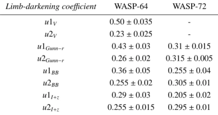
min-imize the correlation of the uncertainties (Holman et al. 2006). To obtain a limb-darkening solution consistent with theory, we used normal prior distributions for u1and u2based on theoretical
values and 1-σ errors interpolated in the tables by Claret (2000; 2004) and shown in Table 4. For our two non-standard filters (I + z and blue-blocking), we estimated the effective wavelength basing on the transmission curves of the filters, the quantum ef-ficiency curve of the camera and the spectral energy distribu-tions of the stars (assumed to emit as blackbodies), and we in-terpolated the corresponding limb-darkening coefficient values in Claret’s tables and estimated their errors by using the values for the two nearest standard filters. We tested the insensitivity of our results to the details of this interpolation by performing short MCMC analyses with different prior distributions for the limb-darkening coefficients of the non-standard filters (e.g. assuming
I + z = I-Cousins, blue-blocking = R-Cousins, etc.) which led to
results fully consistent with those of our nominal analysis. Such tests had also been performed in the past for other WASP plan-ets, with similar results (e.g. Smith et al. 2012).
Limb-darkening coefficient WASP-64 WASP-72
u1V 0.50 ± 0.035 -u2V 0.23 ± 0.025 -u1Gunn−r 0.43 ± 0.03 0.31 ± 0.015 u2Gunn−r 0.26 ± 0.02 0.315 ± 0.005 u1BB 0.36 ± 0.05 0.255 ± 0.04 u2BB 0.255 ± 0.02 0.305 ± 0.01 u1I+z 0.29 ± 0.03 0.205 ± 0.02 u2I+z 0.255 ± 0.015 0.295 ± 0.01
Table 4. Expectation and standard deviation of the normal
dis-tributions used as prior disdis-tributions for the quadratic limb-darkening coefficients u1 and u2 in our MCMC analysis.
Our analysis was composed of five Markov chains of 105
steps, the first 20% of each chain being considered as its burn-in phase and discarded. For each run the convergence of the five Markov chains was checked using the statistical test presented by Gelman and Rubin (1992). The correlated noise present in the light curves was taken into account as described by Gillon et al. (2009b), by comparing the scatters of the residuals in the original and in time-binned versions of the data, and by rescaling the errors accordingly. For the WASP-72 RVs, a ‘jitter’ noise of 5.1 m s−1 was added quadratically to the error bars, to equalize
the mean error with the rms of the best-fitting model residuals. At each step of the Markov chains the dynamical stellar den-sity ρ∗ deduced from the jump parameters (b’, W, (Rp/R∗)2, √e cos ω, √e sin ω, P; see, e.g., Winn 2010) and values for T
eff
and [Fe/H] drawn from the normal distributions deduced from our spectroscopic analysis (Sect. 3.1), were used to determine a value for the stellar mass M∗through an empirical law M∗(ρ∗,
Teff, [Fe/H]) (Enoch et al. 2010; Gillon et al. 2011) calibrated
using the parameters of the extensive list of stars belonging to detached eclipsing binary systems presented by Southworth (2011). For WASP-64, the list was restricted to the 113 stars with a mass between 0.5 and 1.5 M⊙, while the 212 stars with a mass between 0.7 to 1.7 M⊙were used for WASP-72, the goal of this selection being to benefit from our preliminary estimation of the stellar mass (Sec. 3.1, Table 3) to improve the determination of the physical parameters while using a number of calibration stars large enough to avoid small number statistical effects. To propa-gate properly the errors on the calibration law, the parameters of the selected subset of eclipsing binary stars were normally per-turbed within their observational error bars and the coefficients of the law were redetermined at each MCMC step. Using the re-sulting stellar mass, the physical parameters of the system were then deduced from the jump parameters. In this procedure to derive the physical parameters of the system, the spectroscopic stellar gravity is thus not used, the stellar density deduced from the dynamical + transit parameters constraining by itself the evo-lutionary state of the star (Sozzetti et al. 2007). Still, for WASP-72 we assumed a normal prior distribution for log g based on the spectroscopic value and error bar (Table 3), because the low tran-sit depth combined with the significant level of correlated noise of our data led to relatively poor constraint on the stellar density from the photometry alone (error of 50%).
For both systems, two analyses were performed, one assum-ing a circular orbit and the other an eccentric orbit. For the sake of completeness, the derived parameters for both models are shown in Table 5 (WASP-64) and Table 6 (WASP-72), while the
best-fit transit models are shown in Fig. 10 and 11 for the circu-lar model. Using the BIC as proxy for the model marginal like-lihood, the resulting Bayes factors are ∼3000 (WASP-64) and
∼5000 (WASP-72) in favor of the circular models. A circular
orbit is thus favored for both systems, and we adopt the cor-responding results as our nominal solutions (right columns of Table 5 and 6). This choice is strengthened by the modeling of the tidal evolution of both planets, as discussed in Sec. 4.
3.2.1. Stellar evolution modeling
After the completion of the MCMC analyses described above, we performed for both systems a stellar evolution model-ing based on the code CLES (Scuflaire et al. 2008) and on the Levenberg-Marquardt optimization algorithm (Press et al. 1992), using as input the stellar densities deduced from the MCMC, and the effective temperatures and metallicities de-duced from our spectroscopic analyses, with the aim to assess the reliability of the deduced physical parameters and to esti-mate the age of the systems. The resulting stellar masses were 0.95 ± 0.05 M⊙ (WASP-64) and 1.34 ± 0.11 M⊙ (WASP-72),
consistent with the MCMC results, while the resulting ages were 7.0 ± 3.5 (WASP-64) and 3.2 ± 0.6 Gy (WASP-72).
Unlike WASP-64, WASP-72 appears to be significantly evolved. To check further the reliability of our inferences for the system, we derived its parameters using the solar calibrated value of the mixing length parameter and a value 20% lower, and we also investigated the effects of convective core overshooting and microscopic diffusion of helium. All the results are within 1sigma for the mean density and surface metallicity, and within 1.5 sigma for the effective temperature, however the best fits of mean density and Te f f are found for models including con-vective core overshooting. Solutions with standard physics tend to produce mean density higher than 0.2 and Te f f higher than 6300K.
3.2.2. Global analysis of the transits with free timings
As a complement to our global analysis, we performed for both systems another global analysis with the timing of each transit being free parameters in the MCMC. The goal here was to ben-efit from the strong constraint brought on the transit shape pro-vided by the total data set to derive accurate transit timings and to assess the transit periodicity. In this analysis, the parameters
T0 and P were kept under the control of normal prior
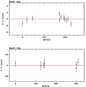
distribu-tions based on the values shown for a circular orbit in Table 5 (WASP-64) and Table 6 (WASP-72), and we added a timing off-set as jump parameter for each transit. The orbits were assumed to be circular. The resulting transit timings and their errors are shown in Table 7. This table also shows (last column) the result-ing transit timresult-ing variations (TTV = observed minus computed timing, O-C). These TTVs are shown as a function of the transit epochs in Fig. 12. They are all compatible with zero, i.e. there is no sign of transit aperiodicity.
4. Discussion
WASP-64 b and WASP-72 b are thus two new very short-period (1.57d and 2.22d) planets slightly more massive than Jupiter or-biting moderately bright (V=12.3 and 10.1) Southern stars. Their detection demonstrates nicely the high photometric potential of the WASP transit survey (Pollacco et al. 2006), as both planets show transits of very low-amplitude (< 0.5%) in the WASP data.
V
Gunn-r
Blue-blocking
I+z
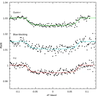
Fig. 10. Combined follow-up transit photometry for WASP-64 b,
detrended, period-folded and binned per intervals of 2 min. For each filter, the best-fit transit model from the global MCMC analysis is superimposed. The V, Gunn-r and blue-blocking light curves are shifted along the y-axis for the sake of clarity.
-0.1 -0.05 0 0.05 0.1 0.99 1 1.01 1.02 1.03 1.04 dT [days] Gunn-r Blue-blocking I+z
Fig. 11. Combined follow-up transit photometry for WASP-72 b,
detrended, period-folded and binned per intervals of 2 min. For each filter, the best-fit transit model from the global MCMC analysis is superimposed. The Gunn-r and blue-blocking light curves are shifted along the y-axis for the sake of clarity.
For WASP-64, the reason is not the intrinsic size contrast with the host star but the dilution of the signal by a close-by spec-troscopic binary that could be dynamically bound to WASP-64 (Sec. 3.1).
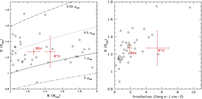
Fig. 13 shows the position of both planets in mass-radius and irradiation-radius diagrams for a mass range from 1 to 2
Fig. 12. TTVs (O − C = observed minus computed timing)
de-rived from the global MCMC analyzes of the WASP-64 b (top) and WASP-72 b (bottom) transits (see Sec. 3.2.1).
Planet Epoch Transit timing - 2450000 O − C [H JDT DB] [s] WASP-64 b 0 5582.60070 ± 0.00051 −85 ± 50 21 5615.64057 ± 0.00057 −19 ± 55 47 5656.54655 ± 0.00035 +15 ± 39 173 5854.78224 ± 0.00027 +97 ± 40 173 5854.78091 ± 0.00032 −19 ± 41 180 5865.79456 ± 0.00025 +35 ± 39 194 5887.82045 ± 0.00035 +18 ± 44 199 5895.68667 ± 0.00029 −5 ± 42 206 5906.69953 ± 0.00041 −19 ± 50 213 5917.71279 ± 0.00019 −1 ± 38 229 5939.73781 ± 0.00030 −92 ± 45 WASP-72 b 0 5583.6542 ± 0.0024 +3.3 ± 5.0 125 5860.7441 ± 0.0048 −0.7 ± 7.7 139 5891.7797 ± 0.0017 +0.9 ± 4.6 143 5900.6475 ± 0.0043 +3.4 ± 8.5 300 6248.6710 ± 0.0029 −5.0 ± 6.4 300 6248.6758 ± 0.0012 +1.8 ± 5.3 309 6268.6292 ± 0.0024 +5.7 ± 6.3
Table 7. Transit timings and TTVs (O − C = observed minus
computed timing) derived from the MCMC global analyzes of the WASP-64 b and WASP-72 b transits.
MJup. WASP-64 b lies in a well-populated area of the irradiation-radius diagram. Its physical dimensions can be considered as rather standard. Its measured radius of 1.27 ± 0.04 RJupagrees
well with the value of 1.22 ± 0.11 RJup predicted by the equa-tion derived by Enoch et al. (2012) from a sample of 71 tran-siting planets with a mass between 0.5 and 2 MJupand relating
planets’ sizes to their equilibrium temperatures and semi-major axes. On the contrary, WASP-72 b appears to be a possible out-lier, its measured radius of 1.27 ± 0.20 RJup being marginally
lower than the value predicted by Enoch et al’s empirical rela-tion, 1.70 ± 0.11 RJup. Its density of 0.732+0.43−0.25ρJupcould indeed
be considered as surprisingly high given its extreme irradiation (∼ 5.5 × 10⁹erg s−1cm−2), suggesting a possible enrichment of heavy elements. Nevertheless, Fig. 13 clearly shows that the er-rors on its physical parameters are still too high to draw any strong inference on its internal structure or its possible peculiar-ity. Indeed, the transit parameters are still loosely determined, especially the impact parameter, resulting in a high relative error on the stellar density that propagates to the stellar and planetary radii. Planets with similar irradiation and mass being still rare, it will thus be especially interesting to improve these parameters with new follow-up observations.
As described in Sec. 3.2, we have adopted the circular or-bital models for both planets, basing on their higher marginal likelihoods. To assess the validity of this choice on a theoretical basis, we integrated the future orbital evolution of both systems through the low-eccentricity tidal model presented by Jackson et al. (2008), assuming as starting eccentricity the 95% upper limits derived in our MCMC analysis (0.132 for WASP-64 b and 0.052 for WASP-72 b) and assuming mean values of 107 and
105 for, respectively, the stellar and planetary tidal dissipation
parameters Q′
∗ and Q′p (Goldreich & Soter, 1966). These inte-grations resulted in circularization times (defined as the time needed to reach e < 0.001) of 4 and 24 Myr for, respectively, WASP-64 b and WASP-72 b. These times are much shorter than the estimated age of the systems, strengthening our selection of the circular orbital solutions. It is worth mentioning that both systems are tidally unstable, as most of the hot Jupiter systems (Levrard et al. 2009), the times remaining for the planets to reach their Roche limits being respectively 0.9 Gy (WASP-64 b) and 0.35 Gy (WASP-72 b) under the assumed tidal dissipation pa-rameters.
The new transiting systems reported here represent both two interesting targets for follow-up observations. Thanks to its ex-treme irradiation and its moderately high planet-to-star size ra-tio, WASP-64 b is a good target for near-infrared occultation (spectro-)photometry programs able to probe its day-side spec-tral energy distribution. Assuming a null albedo for the planet and blackbody spectra for both the planet and the host star, we computed occultation depths of 650-1550 ppm in K-band, 1500-2750 ppm at 3.6 µm and 2050-3350 ppm at 4.5 µm, the lower and upper limits corresponding, respectively, to a uniform redistribu-tion of the stellar radiaredistribu-tion to both planetary hemispheres and to a direct reemission of the dayside hemisphere. Precise measure-ment of such occultation depths is definitely within the reach of several ground-based and space-based facilities (e.g. Gillon et al. 2012). For ground-based programs, the situation is made easier by the presence of a bright (K = 9.8) comparison star at only 28” from the target (Fig. 3). For WASP-72, atmospheric measurements are certainly more challenging considering the lower planet-to-star size ratio. Here, the first follow-up actions should certainly be to confirm and improve our measurement of the planet’s size through high-precision transit photometry, and to gather more RVs to confirm the trend marginally detected in our analysis.
Acknowledgements. WASP-South is hosted by the South African Astronomical Observatory and we are grateful for their ongoing support and assistance. Funding for WASP comes from consortium universities and from UK’s Science and Technology Facilities Council. TRAPPIST is a project funded by the Belgian Fund for Scientific Research (Fond National de la Recherche Scientifique,
F.R.S-Fig. 13. Le f t: mass–radius diagram for the transiting planets with masses ranging from 1 to 2 MJup (data from exoplanet.eu,
Schneider et al. 2011). WASP-64 b and WASP-72 b are shown as red square symbols, while the other planets are shown as open circles without their error bars for the sake of clarity. Different iso-density lines are also shown. Right: position of WASP-64 b and WASP-72 b in a irradiation–radius diagram for the same exoplanets sample.
FNRS) under grant FRFC 2.5.594.09.F, with the participation of the Swiss National Science Fundation (SNF). M. Gillon and E. Jehin are FNRS Research Associates. We thank the anonymous referee for his useful criticisms and sug-gestions that helped us to improve the quality of the present paper.
References
Anderson D. R., Collier Cameron A., Hellier C., et al. 2011, ApJL, 726, L19 Baranne A., Queloz D., Mayor M., et al., 1996, A&AS, 119, 373
Barnes, S. A. 2007, ApJ, 669, 1167
Bruntt, H., Deleuil, M., Fridlund, M., et al. 2010a, A&A, 519, A51 Bruntt, H., Bedding, T. R., Quirion, P.-O., et al. 2010b, MNRAS, 405, 1907 Claret A., 2000, A&A, 363, 1081
Claret A., 2004, A&A, 428, 1001
Collier-Cameron, A., Pollacco, D., Street, R. A., et al. 2006, MNRAS, 373, 799 Collier-Cameron, A., Wilson, D. M., West, R. G., et al. 2007, MNRAS, 380,
1230
Doyle, A. P., Smalley, B., Maxted, P. F. L., et al. 2013, MNRAS, 428, 3164 Enoch, B., Collier-Cameron, A., Parley, N. R., Hebb, L. 2010 A&A, 516, A33 Enoch, B., Collier-Cameron, A. & Horne, K. 2012, A&A, 540, A99 Gelman A., Rubin D., 1992, Statistical Science, 7, 457
Gillon, M., Smalley, B., Hebb, L., et al. 2009a, A&A, 496, 259
Gillon M., Demory B.-O., Triaud A. H. M. J., et al., 2009b, A&A, 506, 359 Gillon, M., Doyle, A. P., Lendl, M., et al. 2011, A&A, 533, A88
Gillon, M., Jehin, E., Magain, P., et al. 2011, Detection and Dynamics of Transiting Exoplanets, Proceedings of OHP Colloquium (23-27 August 2010), eds. F. Bouchy, R. F. Diaz & C. Moutou, Platypus Press, 06002 Gillon M., Triaud A. H. M. J., Fortney J. J., et al. 2012, A&A, 542, 4 Goldreich, O. & Soter, S. 1966, Icarus, 5, 375
Gray, D. F. 2008, The observation and analysis of stellar photospheres, 3rd Edition (Cambridge University Press), p. 507
Hellier, C., Anderson, D. R., Collier-Cameron, A., et al. 2011, Detection and Dynamics of Transiting Exoplanets, Proceedings of OHP Colloquium (23-27 August 2010), eds. F. Bouchy, R. F. Diaz & C. Moutou, Platypus Press, 01004
Holman M. J., Winn J. N., Latham D. W., et al., 2006, ApJ, 652, 1715 Jackson, D., Greenberg, R., & Barnes, R. 2008, ApJ, 678, 1396 Jehin, E., Gillon, M., Queloz, D., et al. 2011, The Messenger, 145, 2 Lammer, H., Odert, P., Leitzinger, M., et al. 2009, A&A, 506, 399
Lendl, M., Anderson, D. R., Collier-Cameron, A., et al. 2012, A&A, 544, A72 Levrard, B., Winisdoerffer, C. & Chabrier, G. 2009, ApJL, 692, 9
Mandel K., Agol E., 2002, ApJ, 580, 181
Mandushev, G., Torres, G., Latham, D. W., et al., 2005, ApJ, 621, 1061
Magain P., 1984, A&A, 134, 189
Maxted, P. F. L., Anderson, D. R., Collier Cameron, A., et al. 2011, PASP, 123, 547
Murray, C. D. & Correia A. C. M. 2010, Exoplanets, edited by S. Seager, University of Arizona Press, p 15-23
Pollacco, D. L., Skillen, I., Collier Cameron, A., et al. 2006, PASP, 118, 1407 Press, W. H., Teukolsly, S. A., Vetterling, W. T., Flannery B. P. 1992,
Numerical recipes in FORTRAN: The art of scientific computing, 2nd Edition (Cambridge University Press)
Queloz D., Henry G. W., Sivan J. P., et al., 2001, A&A, 379, 279 Roeser, S., Demleitner, M., & Schilbach, E. 2010, AJ, 139, 2440 Santos, N., C., Mayor, M., Naef, D., et al. 2002, A&A, 392, 215 Schwarz, G. E. 1978, Annals of Statistics, 6, 461
Schneider, J., Dedieu, C., Le Sidaner, P., et al. 2011, A&A, 532, 79 Scuflaire R., Th´eado S., Montalb´an J., et al. 2008, APSS, 316, 149 Sestito, P. & Randich, S. 2005, A&A, 442, 615
Smith, A. M. S., Anderson, D. R., Collier Cameron, A., et al. 2012, AJ, 143, 81 Southworth, J., 2011, MNRAS, 417, 2166
Sozzetti, A., Torres, G., Charbonneau, D., et al. 2007, ApJ, 664, 1190 Stetson, P. B. 1987, PASP, 99, 111
Torres, G., Konacki, M., Sasselov, D. D., Jha, S. 2005, ApJ, 619, 558 Torres, G., Andersen, J. & Gim´enez, A. 2010, A&A Rev., 18, 67
Winn, J. N. 2010, Exoplanets, edited by S. Seager, University of Arizona Press, p 55-77
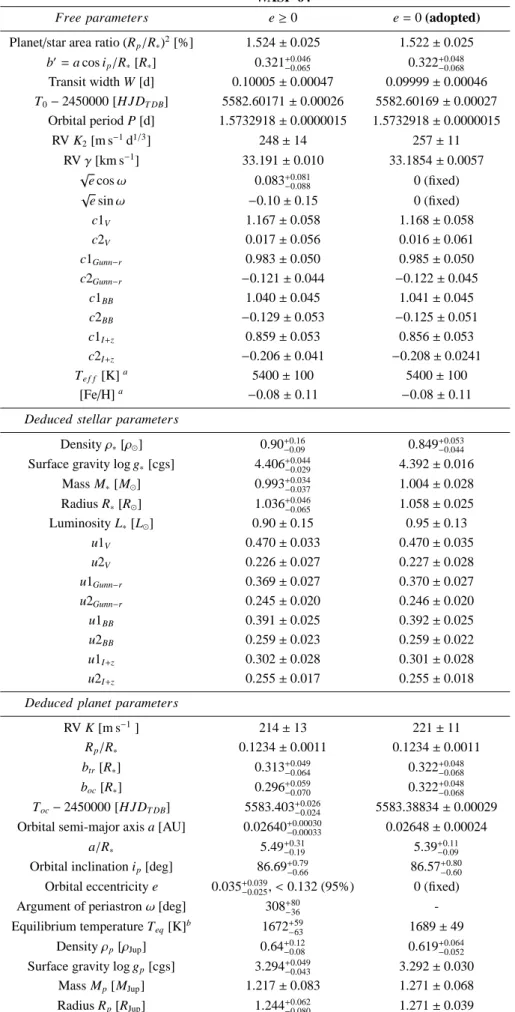
WASP-64
Free parameters e ≥ 0 e = 0 (adopted)
Planet/star area ratio (Rp/R∗)2[%] 1.524 ± 0.025 1.522 ± 0.025 b′= a cos ip/R ∗[R∗] 0.321+0.046−0.065 0.322 +0.048 −0.068 Transit width W [d] 0.10005 ± 0.00047 0.09999 ± 0.00046 T0− 2450000 [HJDT DB] 5582.60171 ± 0.00026 5582.60169 ± 0.00027 Orbital period P [d] 1.5732918 ± 0.0000015 1.5732918 ± 0.0000015 RV K2[m s−1d1/3] 248 ± 14 257 ± 11 RV γ [km s−1] 33.191 ± 0.010 33.1854 ± 0.0057 √ e cos ω 0.083+0.081 −0.088 0 (fixed) √ e sin ω −0.10 ± 0.15 0 (fixed) c1V 1.167 ± 0.058 1.168 ± 0.058 c2V 0.017 ± 0.056 0.016 ± 0.061 c1Gunn−r 0.983 ± 0.050 0.985 ± 0.050 c2Gunn−r −0.121 ± 0.044 −0.122 ± 0.045 c1BB 1.040 ± 0.045 1.041 ± 0.045 c2BB −0.129 ± 0.053 −0.125 ± 0.051 c1I+z 0.859 ± 0.053 0.856 ± 0.053 c2I+z −0.206 ± 0.041 −0.208 ± 0.0241 Te f f[K]a 5400 ± 100 5400 ± 100 [Fe/H]a −0.08 ± 0.11 −0.08 ± 0.11
Deduced stellar parameters
Density ρ∗[ρ⊙] 0.90+0.16
−0.09 0.849
+0.053 −0.044
Surface gravity log g∗[cgs] 4.406+0.044
−0.029 4.392 ± 0.016 Mass M∗[M⊙] 0.993+0.034 −0.037 1.004 ± 0.028 Radius R∗[R⊙] 1.036+0.046 −0.065 1.058 ± 0.025 Luminosity L∗[L⊙] 0.90 ± 0.15 0.95 ± 0.13 u1V 0.470 ± 0.033 0.470 ± 0.035 u2V 0.226 ± 0.027 0.227 ± 0.028 u1Gunn−r 0.369 ± 0.027 0.370 ± 0.027 u2Gunn−r 0.245 ± 0.020 0.246 ± 0.020 u1BB 0.391 ± 0.025 0.392 ± 0.025 u2BB 0.259 ± 0.023 0.259 ± 0.022 u1I+z 0.302 ± 0.028 0.301 ± 0.028 u2I+z 0.255 ± 0.017 0.255 ± 0.018
Deduced planet parameters
RV K [m s−1] 214 ± 13 221 ± 11 Rp/R∗ 0.1234 ± 0.0011 0.1234 ± 0.0011 btr[R∗] 0.313+0.049 −0.064 0.322 +0.048 −0.068 boc[R∗] 0.296+0.059 −0.070 0.322 +0.048 −0.068 Toc− 2450000 [HJDT DB] 5583.403+0.026−0.024 5583.38834 ± 0.00029
Orbital semi-major axis a [AU] 0.02640+0.00030
−0.00033 0.02648 ± 0.00024
a/R∗ 5.49+0.31
−0.19 5.39
+0.11 −0.09
Orbital inclination ip[deg] 86.69+0.79−0.66 86.57+0.80−0.60
Orbital eccentricity e 0.035+0.039
−0.025, < 0.132 (95%) 0 (fixed)
Argument of periastron ω [deg] 308+80
−36
-Equilibrium temperature Teq[K]b 1672+59−63 1689 ± 49
Density ρp[ρJup] 0.64+0.12−0.08 0.619+0.064−0.052
Surface gravity log gp[cgs] 3.294+0.049−0.043 3.292 ± 0.030
Mass Mp[MJup] 1.217 ± 0.083 1.271 ± 0.068
Radius Rp[RJup] 1.244+0.062−0.080 1.271 ± 0.039
Table 5. Median and 1-σ limits of the marginalized posterior distributions obtained for the WASP-64 system parameters as derived
WASP-72
Free parameters e ≥ 0 e = 0 (adopted)
Planet/star area ratio (Rp/R∗)2[%] 0.423+0.039−0.037 0.430 +0.043 −0.039 b′= a cos ip/R ∗[R∗] 0.58+0.10−0.20 0.59 +0.10 −0.18 Transit width W [d] 0.1552 ± 0.0029 0.1558+0.0035 −0.0029 T0− 2450000 [HJDT DB] 5583.6525 ± 0.0021 5583.6529 ± 0.0021 Orbital period P [d] 2.2167434+0.0000084 −0.0000077 2.2167421 ± 0.0000081 RV K2[m s−1d1/3] 236.6 ± 5.6 236.1 ± 5.5 RV γ [km s−1] 35.923 ± 0.015 35.919 ± 0.014 RV slope [m s−1y−1] −44 ± 19 −39 ± 17 √ e cos ω −0.022 ± 0.071 0 (fixed) √ e sin ω −0.06 ± 0.11 0 (fixed) c1Gunn−r 0.938 ± 0.026 0.936 ± 0.026 c2Gunn−r −0.318 ± 0.016 −0.319 ± 0.017 c1BB 0.820 ± 0.082 0.818 ± 0.078 c2BB −0.352 ± 0.046 −0.352 ± 0.042 c1I+z 0.713 ± 0.041 0.710 ± 0.042 c2I+z −0.382 ± 0.028 −0.383 ± 0.027 Te f f[K]a 6250 ± 100 6250 ± 100 [Fe/H]a −0.06 ± 0.09 −0.06 ± 0.09
Deduced stellar parameters
Surface gravity log g∗[cgs]a 3.99 ± 0.10 3.99+0.10 −0.11 Density ρ∗[ρ⊙] 0.181+0.074 −0.046 0.177 +0.073 −0.048 Mass M∗[M⊙] 1.382 ± 0.053 1.386 ± 0.055 Radius R∗[R⊙] 1.97 ± 0.23 1.98 ± 0.24 Luminosity L∗[L⊙] 5.3+1.4 −1.2 5.3 +1.5 −1.3 u1Gunn−r 0.311 ± 0.013 0.311 ± 0.013 u2Gunn−r 0.3148 ± 0.0063 0.3147 ± 0.0060 u1BB 0.257 ± 0.043 0.256 ± 0.041 u2BB 0.305 ± 0.013 0.305 ± 0.014 u1I+z 0.209 ± 0.022 0.208 ± 0.022 u2I+z 0.295 ± 0.012 0.295 ± 0.013
Deduced planet parameters
RV K [m s−1] 181.3 ± 4.2 181.0 ± 4.2 Rp/R∗ 0.0650 ± 0.0029 0.0656 ± 0.0031 btr[R∗] 0.57+0.10 −0.20 0.59 +0.10 −0.18 boc[R∗] 0.58+0.11 −0.21 0.59 +0.10 −0.18 Toc− 2450000 [HJDT DB] 5584.758 ± 0.042 5584.7612 ± 0.0021
Orbital semi-major axis a [AU] 0.03705 ± 0.00047 0.03708 ± 0.00050
a/R∗ 4.05+0.49
−0.38 4.02
+0.49 −0.40
Orbital inclination ip[deg] 81.8+3.5−2.5 81.6+3.2−2.6
Orbital eccentricity e 0.014+0.018
−0.010, < 0.079 (95%) 0 (fixed)
Argument of periastron ω [deg] 115+111
−47
-Equilibrium temperature Teq[K]b 2200+110−120 2210+120−130
Density ρp[ρJup] 0.75+0.45−0.25 0.72+0.43−0.25
Surface gravity log gp[cgs] 3.37+0.13−0.11 3.36 ± 0.12
Mass Mp[MJup] 1.459 ± 0.056 1.5461+0.059−0.056
Radius Rp[RJup] 1.25 ± 0.19 1.27 ± 0.20
Table 6. Median and 1-σ limits of the marginalized posterior distributions obtained for the WASP-72 system parameters as derived
from our MCMC analysis.aUsing as priors the spectroscopic values given in Table 3.bAssuming a null Bond albedo (AB=0) and isotropic reradiation ( f =1/4).