The InSight Blind Test: An Opportunity to Bring a Research Dataset into Teaching Programs

(1)

HAL Id: hal-02461538

https://hal.archives-ouvertes.fr/hal-02461538

Submitted on 24 Nov 2020

HAL is a multi-disciplinary open access archive for the deposit and dissemination of sci-entific research documents, whether they are pub-lished or not. The documents may come from teaching and research institutions in France or abroad, or from public or private research centers.

L’archive ouverte pluridisciplinaire HAL, est destinée au dépôt et à la diffusion de documents scientifiques de niveau recherche, publiés ou non, émanant des établissements d’enseignement et de recherche français ou étrangers, des laboratoires publics ou privés.

The InSight Blind Test: An Opportunity to Bring a

Research Dataset into Teaching Programs

Julien Balestra, Jean-Luc Berenguer, Florence Bigot-cormier, Françoise

Courboulex, Lucie Rolland, David Ambrois, Martin van Driel, Philippe

Lognonne

To cite this version:

Julien Balestra, Jean-Luc Berenguer, Florence Bigot-cormier, Françoise Courboulex, Lucie Rolland, et al.. The InSight Blind Test: An Opportunity to Bring a Research Dataset into Teaching Pro-grams. Seismological Research Letters, Seismological Society of America, 2020, 91 (2A), pp.1064-1073. �10.1785/0220190137�. �hal-02461538�

(2)

1

The InSight Blind Test: an Opportunity to Bring a Research Dataset into Teaching 1

Programs 2

3

Julien Balestra(1)_{, Jean-Luc Berenguer}(2,3)_{, Florence Bigot-Cormier}(4)_{, Françoise Courboulex}(2)_, 4

Lucie Rolland(2), David Ambrois(2), Martin Van Driel(5) and Philippe Lognonné(6)

5

6

1) Université Côte d’Azur, Campus Valrose, Bâtiment L, 28 Avenue de Valrose, 06108 Nice

7

CEDEX 2, France

8

2) Université Côte d’Azur, CNRS, Observatoire de la Côte d’Azur, IRD, Géoazur, UMR7329,

9

250 rue Albert Einstein, Sophia Antipolis 06560 Valbonne, France

10

3) Centre International De Valbonne, BP 97, 06902 Sophia Antipolis, Cedex, France

11

4) French School of Shanghai, 350 Gao Guang Road, Qingpu District, Shanghai 201702, China

12

5) Institute of Geophysics, ETH Zürich, Sonneggstrasse 5, 8092, Zurich, Switzerland

13

6) Université de Paris, Institut de physique du globe de Paris, CNRS, F-75005 Paris, France

14

15

Corresponding author: julien.balestra@univ-cotedazur.fr

16 17 18 19 20 21

(3)

2 Abstract

22

On November 26, 2019, SEIS, the first broadband seismometer designed for the Martian

23

environment (Lognonné et al., 2019) landed on Mars thanks to NASA’s InSight mission. On

24

April 6, 2019 (sol 128), the InSight Science team detected the first historical “marsquake”

25

(NASA news release). Before it was recorded, the InSight Science team developed the InSight

26

Blind Test (hereafter IBT), which consists of a 12-month period of continuous waveform data

27

combining realistic estimates of martian background seismic noise, 204 tectonic and 35 impact

28

events (Clinton et al., 2017). This project was originally designed to prepare scientists for the

29

arrival of real data from the upcoming InSight mission. This paper presents the work carried

30

out by middle and high school students during this challenge. This project offered schools the

31

opportunity to participate in and strengthen the link between secondary schools and universities.

32

The IBT organizers accepted the approach to enable fourteen schools to take part in this

33

scientific challenge. After a training process, each school analyzed the IBT dataset to contribute

34

to the collaborative School Team catalog. The schools relied on a manual procedure combining

35

analyses in time and frequency domains. At the end, a combined catalog was submitted as one

36

of the IBT entries. The IBT organizers then assessed the catalog submitted by the consortium

37

of schools together with the results from science teams (Van Driel et al., 2019). The schools

38

achieved a total of 15 correct detections over a short period. While this number may seem

39

modest compared with the 239 synthetic marsquakes included in the IBT waveform data, these

40

correct detections were entirely made during class time. All in all, the students seemed to be

41

fully engaged, and this exercise seemed to increase their scientific inquiry skills in order to

42

fulfill their task as a team.

43

44

(4)

3 Introduction

46

The InSight mission includes an education and outreach program (E&O) in each partner

47

country. In France, the E&O is carried out by the Géoazur education team. Many pedagogical

48

resources were proposed for this mission, including aspects from launch to landing. The IBT

49

was an excellent opportunity to prepare students to work on future Martian seismograms. The

50

organizers prepared a synthetic dataset of continuous waveforms and invited participants to

51

detect both tectonic and impact seismicity, along with different sources of noise (Murdoch et

52

al., 2017a, 2017b, Kenda et al., 2017). Note that:

53

- the IBT stopped on February 2018,

54

- the continuous synthetic signal was considered for a fictional year 2019 (from January

55

1 to December 31).

56

All mentions of data from 2019 concern this fictional year.

57

The objective was to prepare research teams interested in developing detection procedures and

58

assess the quality of their work by comparing the seismicity catalog they produced with the IBT

59

synthetic seismicity catalog.

60

Given that using data in schools from scientific research has shown a positive impact on

61

students (Zollo et al., 2014, Bigot-Cormier and Berenguer, 2017), we asked the IBT organizers

62

if the participation of schools was possible. We proposed having the students determine key

63

event parameters such as date, arrival time of seismic waves, epicentral distance and

back-64

azimuth direction, terms used in the French educational curriculum. The organizers accepted

65

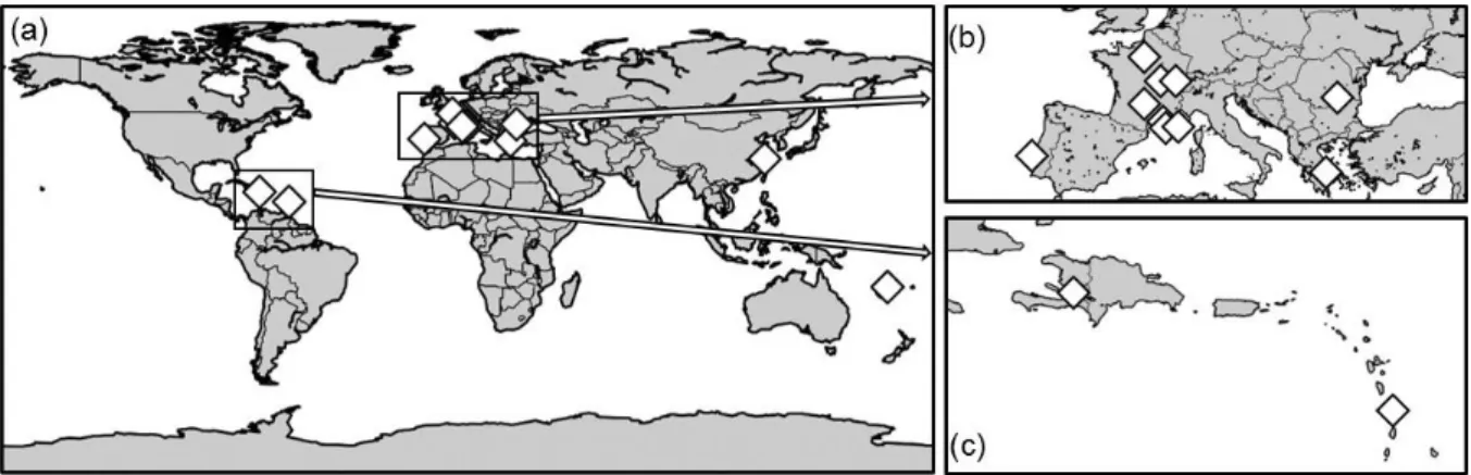
this format. The School Team was composed of 14 schools either in France or abroad (Fig. 1),

66

all of which are part of the French educational seismic network (Courboulex et al., 2012). Catts

67

Pressoir Middle School is a Haitian school, but their teaching program is similar to that of the

68

French curriculum followed by the other schools. The IBT was considered to be an excellent

(5)

4

scientific dataset for teaching lessons and was aligned with a series of expected skills, which

70

will be highlighted throughout this study.

71

One of the expected skills is to identify, extract and organize information from scientific data.

72

In middle school lessons, earthquakes are taught as being the result of the Earth’s internal

73

activity. Students learn that ground motions during an earthquake are due to different waves

74

shaking the surface. A typical class exercise is to identify different seismic phases in a

75

seismogram. During subsequent high school lessons, a classic exercise is to determine the

76

arrival times of seismic P and S waves in order to locate the epicenter. We were strongly

77

convinced that the data from the IBT could be used instead of these classic exercises as a

78

previously unseen dataset. Furthermore, it was felt that student motivation would be increased

79

by knowing that the InSight science team would analyze their results.

80

At the start of this project, a training process was required to efficiently prepare students for the

81

upcoming synthetic data analysis.

82

83

Student Training Process 84

Real Earth and Synthetic Mars Data

85

In order to train students and increase their skills in seismic signal analysis, we provided

86

students with two newsletters in October 2017. Each document was in PDF format, with

87

numerical data attached. In this study, all numerical datasets were analyzed with

88

SeisGram2K80_ECOLE.jar (SG2K80, Lomax A., 2000) software. A specific velocity model

89

was implemented by A. Lomax (from Sohn and Spohn, 1997).

90

The task approach was to study examples of signal processing. Students first worked on

91

decimation and its effect on seismic data. We provided real seismograms recorded at the BLOR

(6)

5

education station (“Lycée de la Montagne” high school in Valdeblore, France). The earthquakes

93

considered were:

94

- the April 7, 2014, Barcelonnette earthquake (Mw 4.9, France, 0.6° epicentral

95

distance);

96

- the April 16, 2016, earthquake (Mw 7.8, Ecuador region, 87.6° epicentral distance).

97

Students then worked on bandpass filtering and frequency content. We provided synthetic

98

signals from the IBT. The proposed fictional time periods were:

99 - January 10 to 15, 2019; 100 - July 15, 2019; 101 - September 22, 2019. 102

We rotated these signals into the north, east, and Z (vertical) directions from metadata provided

103

by the IBT organizers using the ObsPy packages (Krischer et al., 2015). No instrumental

104

correction for response was applied.

105

106

Decimation of Seismic Signals: an Exercise to Manipulate, Experiment, and Understand the

107

Nature of the Data Used

108

The first exercise was designed to help students become familiar with the nature of the IBT

109

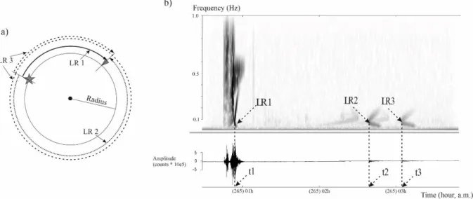
dataset, especially with the difficulty of working with decimated seismic data. The SEIS

110

seismometer stores data at 100 Hz. At the time of the IBT, the initial sampling rate retained for

111

future real data transmission was 2 Hz. This corresponds to a volume of data transfer

112

guaranteed by the NASA. The educational seismic stations used by students typically store

113

ground motion at 50 Hz. Therefore, the first exercise was to introduce the synthetic data

114

corresponding to decimated data, i.e. with lower resolution than the raw data. Students worked

(7)

6

on the Barcelonnette earthquake decimated to 2 Hz. Decimation was carried out using the

116

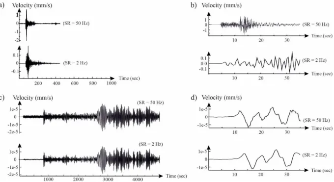
Python ObsPy software package (with an anti-aliasing low-pass filter). Figure 2a shows raw

117

and decimated seismograms (vertical component). Change in amplitude was the first effect

118

observed by students. They understood that samples were missing, which implies that

119

information about ground motion was missing. Zooming in with SG2K80 also allowed them to

120

observe changes in shape (Fig. 2b). After these first manipulations, students worked on the

121

teleseismic event. At first they observed no significant changes in amplitude between the raw

122

and the decimated signal (Fig. 2c). They observed that the decimation had very little effect on

123

the signal. Zooming in enabled them to observe small differences due to the anti-aliasing

124

prefiltering (Fig. 2d).

125

This first analysis of changes of seismogram shapes enabled students to understand the effect

126

of this kind of processing on raw data. Understanding the link between the content of a dataset,

127

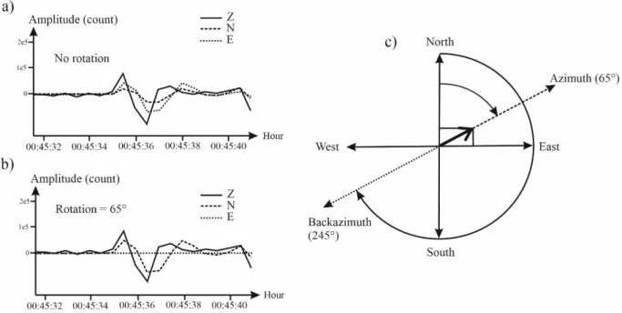
and the information that can be extracted from it, is an important skill required in French

128

educational programs. Moreover, students were also able to imagine how difficult it would be

129

to analyze future real Martian seismograms decimated to 2 Hz.

130

This first step concluded with the introduction of the relationship between the shape and period

131

of the signal. Signals were described as being composed of tighter or looser arcs, with tight arcs

132

corresponding to short periods and broad arcs corresponding to long periods, following the

133

approach of Bigot-Cormier and Berenguer (2017). This allowed us to introduce a second step

134

based on frequency analysis.

135

136

Bandpass Filter and Spectrogram: Use of Digital Tools to Identify Seismic Waves

137

The frequency content of seismograms was introduced in response to the question raised by

138

students: “How will scientists be able to detect seismic activity?”. For both middle and high

(8)

7

school students, the use of a bandpass filter is unusual. Understanding the calculation of

140

spectrograms is too difficult, and it is not a subject in the French curriculum. However, students

141

are expected to use digital processing software. SG2K80 proposes tools to filter seismograms

142

and to compute a corresponding spectrogram, which was introduced as a data processing

143

method to highlight the frequency content of the continuous signals. To become familiar with

144

these different aspects, students were invited to work with the synthetic seismogram on January

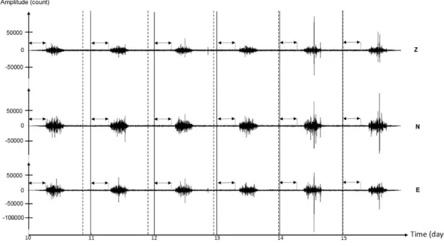
145

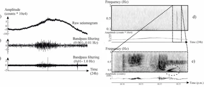
12, 2019 (IBT fictional day, vertical component, Fig. 3). Note that any mentions below of a

146

synthetic seismogram refer to the IBT, except seismograms computed in the study of Bozdağ

147

et al. (2017).

148

Students started this new activity by applying bandpass filters to understand their effects on the

149

seismograms analyzed. Two frequency intervals were provided:

150

- from 0.001 Hz to 0.01 Hz (lf-bp for low frequencies bandpass),

151

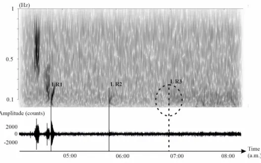
- from 0.01 Hz to 1.0 Hz (hf-bp for high frequencies bandpass).

152

The frequency of 1 Hz corresponds to the Nyquist frequency, i.e. the maximum frequency that

153

can be analyzed for a decimation to 2 Hz. The comparison of these three signals (raw and

154

filtered) allowed students to highlight different points of the filtering process. By applying

lf-155

bp filtering, they observed that the very long period arc observed in Figure 3a was filtered out.

156

They also observed a long duration event (Fig. 3b). With hf-bp filtering this long duration event

157

was always observed along with a later and shorter duration event (Fig. 3c).

158

This kind of processing is consistent with the skills required by the educational curriculum.

159

Students showed they understood that:

160

- events (seismic, atmospheric, etc.) observed in a seismogram have their own frequency

161

characteristics;

(9)

8

- the filtering process is used to try to highlight expected or searched events in

163

seismograms;

164

- the shape of seismograms varies according to removed frequencies.

165

Although, in this case, a filtering process allows the detection of significant events, we invited

166

students to analyze the computed spectrogram from the raw seismogram (SG2K80 spectrogram

167

tool, Fig. 3d and 3e). Students observed that the long and later short events are easier to detect

168

by displaying the frequency content of the seismogram reading. Figure 3d shows that the two

169

events are highlighted by an increased amplitude for specific frequencies (about 0.1 Hz for the

170

long event, up to 0.8 Hz for the shorter event), which indicates a significant change in ambient

171

ground motion.

172

Students understood that hidden synthetic marsquakes could be easier to detect by processing

173

data. To go even deeper into the analysis, zooming in on the late and short event was proposed

174

(Fig. 3e). Students observed that the long duration signal is composed of a frequency content

175

different from the shorter duration event. They also observed an extended coma-like shape (Fig.

176

3e, black dashed ellipse). From discussions with seismologists at Géoazur (who also

177

participated in the IBT as one of the challengers, Van Driel et al., 2019), this specific shape was

178

designated as the signature of Rayleigh waves. These surface waves have a velocity that is

179

dependent on their frequencies. Thus, some Rayleigh waves arrive earlier and some arrive later,

180

which reflects their dispersion. This specific shape was used to determine and identify them.

181

The frequency content of body waves was also approached. From the July 15 (M4.3) and the

182

September 22 (M5.0) synthetic events, the frequency content of body waves was considered as

183

ranging from 0.3 Hz to 0.9 Hz (higher than the frequency content of Rayleigh waves). The work

184

on seismic phases with these large synthetic events was considered as sufficient to help students

185

to detect smaller nearby quakes with higher frequency content.

(10)

9

The training process stopped here for middle school students. According to their educational

187

curriculum, they were ready to analyze synthetic data. Their goal was to identify arrival times

188

of seismic waves and to propose their part of the School Team catalog of seismicity. It was

189

possible to extend this analysis for high school students, thus the second newsletter was given

190

to them.

191

192

Guided Analysis and Interpretation of Synthetic Signals from the InSight Blind Test: Skills

193

Expected for High School Students

194

A. Estimation of the epicentral distance based on Rayleigh wave arrival times

195

Extracting information from scientific datasets is an expected skill for high school students.

196

Locating the epicenter is a good exercise for this, and even more so if the dataset comes from a

197

current scientific project. Typically, seismic events are located by analyzing P and S wave

198

arrival times from three or more seismic stations. One aim of the second newsletter given to

199

students was to introduce a location technique using only one three-component station, without

200

any knowledge of an accurate deep structure of the planet, and without the origin time. We

201

proposed using successive Rayleigh wave arrival times (Panning et al., 2015). Hereafter this

202

paper will use the following notations (Fig. 4a and 4b):

203

- t1: the first arrival time of Rayleigh waves at the virtual station, i.e. the shortest surface

204

travel time between the epicenter and the station (LR1, for Long-period Rayleigh 1);

205

- t2: the second arrival time of Rayleigh waves at the station, i.e. the longest surface travel

206

time between the epicenter and the station (LR2);

(11)

10

- t3: the third arrival time of Rayleigh waves at the station, i.e. the shortest surface travel

208

time between the epicenter and the station, plus a complete surface trip around the planet

209

(LR3).

210

The method from Roques et al. (2016) was used to illustrate this approach (Fig. S1). The

211

synthetic seismograms used in this method came from the study by Bozdağ et al. (2017). They

212

were computed at virtual stations along the Mars equator, spaced by 20°. The mathematical

213

formula to compute epicentral distance from t1, t2, and t3 arrival times is:

214

𝐸𝑝𝑖𝑐𝑒𝑛𝑡𝑟𝑎𝑙 𝑑𝑖𝑠𝑡𝑎𝑛𝑐𝑒 = 𝑡3−𝑡2

𝑡3−𝑡1∗ 𝜋 ∗ 𝑅𝑝𝑙𝑎𝑛𝑒𝑡 (1) 215

where 𝑅𝑝𝑙𝑎𝑛𝑒𝑡 is the radius of the considered planet. Distances are in kilometers and arrival 216

times are in seconds. This work was interesting because distances and origin times were known.

217

Students were easily able to confirm their results.

218

We then invited students to work with an unknown event from the IBT using the synthetic

219

seismogram from September 22, 2019 (Fig. 4b). We chose this event because the analysis of its

220

frequency content showed specific signatures considered as a marker of Rayleigh waves.

221

Students were able to observe the different wave trains in the time domain, which presented

222

specific signatures in the frequency domain. From this analysis and by picking the three

223

passages of Rayleigh waves, students estimated an epicenter located at 35.5° from the station.

224

Thus they understood that this approach is not enough to locate the event. They estimated a

225

distance, but the direction was missing. This aspect was the subject of the last training exercise.

226

227

B. Azimuth and back-azimuth estimation from the rotation of horizontal components

228

This last exercise was introduced using a simple hands-on activity. We provided electronic

229

accelerometers and the RISSC© (Record Interface Sensors at School, see Data and Resources)

(12)

11

interface. This educational interface displays records from each component in real time, which

231

are identified with a sticky label (Fig. S2). The accelerometers were fixed on a table, and

232

students followed two procedures: first, to apply an impact parallel to the table plane in the X

233

direction of the device, and second, to apply an impact in the Y direction of the device. Using

234

records displayed with RISSC, students observed the difference in amplitude of each

235

component and concluded that the maximum amplitude is observed in the main direction of

236

wave propagation. In class, students then reviewed the relationship between azimuth and

back-237

azimuth. SG2K80 software includes a tool to compute the angle value of the azimuth from the

238

first P wave amplitude on horizontal components (Fig. 5). This function allows recomputed

239

signals to be displayed after a chosen rotation value (as a virtual rotation of the sensor in the

240

geographical coordinate system). Figure 5a shows the first P wave on each component, without

241

rotation. Figure 5b shows a flat P wave on the East component for a 65° (clockwise) rotation.

242

This is also the value for which the P wave amplitude is maximal on the North component.

243

Students understood that this virtual rotation of the sensor allows them to determine the

244

direction for which the first ground motion is maximal on one of the horizontal components

245

and zero on the other.

246

The last training exercise involved determining the back-azimuth. From the P wave polarity

247

(upwards) on the vertical component, students calculated a back-azimuth equal to 245°. The

248

final catalog of the IBT was not available at the moment of this training process. Students waited

249

for the publication of the solution to evaluate their first detection. Figure S3 shows the results

250

of this training exercise validated after the publication of the true catalog. They used the

251

EduCarte-Mars geographical information system (GIS) to display the results of location. The

252

specific Mars digital field model was implemented by A. Lomax.

(13)

12

This last activity completed the schools’ training for the IBT. The fourteen schools then each

254

received one month of non-overlapping synthetic data and started their analyses during their

255

teaching sessions.

256

257

Blind Test Independent Data Analysis and the Creation of the School Team Catalog 258

The analysis phase started at the beginning of November, 2017, and ended in January, 2018.

259

This period was long enough for teachers to integrate this challenge (training and analysis

260

phases) into their official teaching hours. Students worked for six to ten hours on this project.

261

We now describe two activities performed by students at each school.

262

263

A Daily Atmospheric Signature

264

During the one-year-long synthetic seismogram, disturbances in the continuous signal were not

265

exclusively due to traveling seismic waves. For example, environmental noise (Spiga et al.

266

2010) was added in order to create a signal that was as realistic as possible (Clinton et al., 2017),

267

with the associated modeled seismic noise originating from the interaction of the environment

268

with the lander or the ground (Murdoch et al, 2017a, 2017b, Kenda et al., 2017). See Spiga et

269

al. (2018) for a general review of atmospheric seismic noise and Lognonné et al. (2019) for

270

noise shielding on the SEIS instrument.

271

During the training steps, students identified an unknown long event in the synthetic

272

seismogram that occurred on January 12, 2019 (fictional day from the IBT). During the analysis

273

phase, students observed that in fact this long event occurred each day, but not at the same hour.

274

Students asked us for an explanation of this phenomenon, and we submitted the question to a

275

researcher, who gave them the following explanation. The sun warms the surface of Mars,

(14)

13

which causes thermal agitation (convection) near the surface. At nightfall, the surface cools

277

because the sun no longer warms it and convection stops. The wind blows, but there are no

278

rapid turbulent fluctuations that produce this atmospheric noise. The observed time lag can be

279

explained by the length of Martian days, which last approximately 24 hours and 39 minutes.

280

One of our aims was reached through this interaction, i.e. to create a link between students and

281

researchers, and to improve the students’ scientific inquiry skills.

282

283

Estimation of the Epicentral Distance of an Unknown Event That Occurred on July 15, 2019

284

This section presents the analysis provided by high school students of the event of July 15, 2019

285

(fictional day from the IBT). They were able to observe different wave trains on the vertical

286

component and they clearly identified two Rayleigh wave signatures in the frequency domain

287

(Fig.7). However, without a clear third signature from the whole day’s seismogram, they

288

decided to pick a third Rayleigh wave at the start of an increase of the scale amplitude around

289

7:00 a.m. By picking these three Rayleigh waves, they obtained an epicentral distance equal to

290

90.5° (from the corresponding SG2K80 tool). The correct epicentral distance was 90.94°. The

291

slight change in amplitude in the frequency domain is probably due to the start of daily

292

atmospheric disturbances, but the lower value of the bandpass filter value applied by students

293

(0.1 Hz to 1 Hz, Fig. 7) was too high to highlight this daily event. However, we appreciated

294

their approach and their thinking through the use of the analysis processes they learned during

295

the training phase.

296

297

298

(15)

14 Discussion

300

The teachers’ geophysical skills enabled the project to be properly completed. They have

301

attended various workshops on the subject during their careers and have already worked on

302

educational projects based on seismic data. The teachers included this challenge in their

303

teaching time and at their convenience. As mentioned above, the students worked at most about

304

ten hours. The schools worked independently during the analysis phase. The main reason for

305

this was that teachers chose the allocated period to work on synthetic data. At the end of January

306

2018, the catalog from the School Team was provided to the IBT organizers. This catalog

307

(Table 1) was then compiled in Van Driel et al. (2019) (Fig. S4). The School Team catalog

308

contained fifteen correct events: thirteen quakes and two impacts. Six high schools and two

309

middle schools found these events. The other schools gave wrong detections. For the students,

310

the main constraints were the available tools and the limited time to work on this challenge.

311

Detected events were located between 700 km and 8400 km from the chosen seismometer

312

location. The detected synthetic events had magnitudes ranging from 2.5 to 5. The closest event

313

in the true catalog (191 km, M2.5) was not detected. Two events of magnitude 2.5 and 2.6 were

314

detected. Their epicentral locations were 724 km and 713 km respectively. Seven events,

315

ranging from magnitude 3 to magnitude 4, were detected. Their epicentral locations ranged

316

from 1000 km to 6500 km. One event with a magnitude higher than 4 was detected (at 5379

317

km). The larger event (M5.0, 2000 km) occurred on September 22 (studied during the training

318

process) was also added to the catalog. Two impacts were also detected, the stronger impact on

319

October 24, and a weaker impact on October 25.

320

In total, 103 events were compiled in the School Team catalog. Changes in the amplitude and

321

frequency of the continuous signal often were considered as seismic waves, because the

322

corresponding computing spectrogram showed changes in amplitudes. These false detections

323

could be a result of the very short teaching time allowed in the training and analysis phases.

(16)

15

These many false detections could be the starting point for a new educational project with a

325

dataset from the IBT. Future student groups could start analyzing why these false detections

326

were made. The aim would be to improve the training phase documentation in order to facilitate

327

the dismissal of some events in the continuous signal.

328

This study could be conducted once again at middle schools and high schools, which could be

329

paired. Middle school students would work on identifying seismic waves, and the high school

330

students would have two objectives: i) validate or invalidate detections, ii) try to estimate a

331

location for detections considered as true. This networking would allow for an increase of

332

educational skills. Furthermore, annual educational projects are planned in new educational

333

programs for high schools. A longer period to work on this challenge would be useful to enable

334

us to compare the quality of the catalog provided.

335

336

Conclusion 337

Of course, our ambition was not to compete with other science teams. Our main goal was to

338

highlight the IBT dataset to school students. This objective was achieved because of motivated

339

teachers who decided to engage their students in this challenge. No written evaluation was

340

specifically carried out, but all teachers reported their satisfaction with the work provided by

341

students. They were also satisfied that they had been able to include this dataset in their own

342

activities. Figures S5a and S5b show pictures of students working on this challenge. Even the

343

few students with learning difficulties responded well to the project, showing a good level of

344

involvement and were engaged in class discussions. We think that the reason was that the

345

framework was out of the ordinary. The aim was not to work on a typical exercise, but to suggest

346

a catalog to the InSight Science Team.

(17)

16

Teacher feedback focused on the great impact of the IBT on classroom dynamics. It allowed

348

students to develop the following main skills:

349

- practice a scientific approach;

350

- demonstrate observation skills, curiosity, critical thinking;

351

- experience autonomy;

352

- communicate in scientifically appropriate language: oral, written, graphic, numerical.

353

Middle school students showed that they were able to detect synthetic events, even though their

354

scientific background was less developed than that of high school students. This point highlights

355

that involvement and seriousness, and not the age of students, were the main determining

356

aspects to properly carry out this challenge.

357

The French EduMed Observatory educational project organized a seminar in the French

358

Géoazur laboratory. Students from high schools came to present the classwork they had carried

359

out during their school year. One group presented their work from the September 22 synthetic

360

quake (Fig. S5c). They presented their picks of Rayleigh waves and their estimate of the

361

epicentral location. They also presented their work on 1D velocity models proposed for the IBT

362

(Clinton et al., 2017). They estimated the origin time from t1, t2, and t3, and then they calculated

363

the velocity of the first P wave. They also considered the following starting models: i) a

364

homogeneous planet, ii) the source located at the surface, iii) a seismic ray as a straight line

365

between the source and the station. They also computed a theoretical depth reached by this first

366

“straight” P wave. By comparing their results with velocity models published in Clinton et al.

367

(2017), they understood that they had chosen a wrong starting velocity model, and learned about

368

how seismic datasets are used to understand the deep structure of Mars. Although they did not

369

succeed in determining the model that was used for the IBT, they showed that they developed

370

many expected skills by working on this dataset.

(18)

17

Student teams are now ready and looking forward to analyzing real data from Mars. In addition,

372

educators should keep in mind that even more challenging seismic signals are expected to be

373

recorded on Mars, with a majority of small, nearby marsquakes (higher frequency content,

374

lower signal noise ratio). A couple of teleseismic events will hopefully reveal the deep interior

375

of the planet.

376

377

Data and Resources 378

Seismograms from the two earthquakes recorded at the BLOR educational seismic station,

379

SeisGram2K80_ECOLE.jar software, and the RISSC interface are available on the EduMed

380

Observatory website:

381

- the Barcelonnette earthquake:

382

http://edumed.unice.fr/fr/data-center/seismo/donnees-seismo/2014-04-07-5_0_barcelonnette

383

- The Ecuador earthquake:

384 http://edumed.unice.fr/fr/data-center/seismo/donnees-seismo/2016-04-16-7_8_ecuador 385 - SG2K80: 386 http://edumed.unice.fr/fr/contents/news/tools-lab/SeisGram2K 387

- Record Interface Sensors at School (developed by David Ambrois):

388

http://edumed.unice.fr/fr/contents/news/tools-lab/RISSC

389

390

EduMed Observatory is funded by the University of Côte d’Azur – JEDI Investments in the

391

Future project managed under reference number ANR-15-IDEX-01.

(19)

18

Synthetic seismograms for the IBT are available from the specific ETH website

393

(http://blindtest.mars.ethz.ch).

394

The synthetic data presented in this study and EduCarte software (Mars version) are also

395

available on the French InSight educational website supported by the Centre National d’Etudes

396

Spatiales (CNES):

397

- InSight Blind Test dataset:

398

https://insight.oca.eu/images/InSight_Medias/zip/blindtest_daily_synthetic_data.zip

399

- Synthetic data from Bozdağ et al. (2017):

400

https://insight.oca.eu/images/InSight_Medias/zip/data/data-bozdag-2017.zip

401

- EduCarte Mars (© A. Lomax and J.L. Berenguer):

402 https://insight.oca.eu/images/InSight_Medias/zip/software/Educarte-Mars-3.3.0X18.zip 403 404 Acknowledgments 405

We are especially grateful to the IBT organizers for accepting a School Team in their challenge

406

and to have provided their dataset. We are also grateful for the help from our scientist partners:

407

Anne Deschamps, Fabrice Peix, Jérôme Chèze (Laboratoire Géoazur), and Aymeric Spiga

408

(Laboratoire de Météorologie Dynamique) for their help and support. InSight Education

409

activities are supported by CNES. This is InSight contribution number: ICN 97. We also are

410

grateful to the reviewers, and especially to Jennifer Hecker for reviewing the English language

411

and grammar used.

412

413

(20)

19 References

415

Bigot-Cormier Florence and Jean-Luc Berenguer (2017). How students Can Experience

416

Science and Become Researchers: Tracking MERMAID Floats in the Oceans.

417

Seismological Research Letters, Volume 88, Number 2A, doi:10.1785/0220160121.

418

Bozdağ, E., Y. Ruan, N. Metthez, A. Khan, K. Leng, M. van Driel,…, and B.W. Banerdt (2017).

419

Simulations of Seismic Wave Propagation on Mars. Space Science Review, Volume

420

211, Issue 1-4, pp 571-594, doi:10.1007/s11214-017-0350-z

421

Clinton, J., D. Giardini, P. Lognonné, B.W. Banerdt, M. Van Driel, M. Drilleau, … , and A.

422

Spiga (2017). Preparing for InSight: An Invitation to Participate in a Blind Test for

423

Martian Seismicity. Seismological Research Letters, 88.5, pp. 1290-1302,

424

doi:10.1785/0220170094.

425

Courboulex, F., J.L. Berenguer, A. Tocheport, M.P Bovin, E. calais, Y. Esnault, … , and J.

426

Virieux (2012). SISMOS à l’Ecole : A Worldwide Network of Realtime Seismometers

427

in Schools. Seismological Research Letters, volume 83, number 5, September/October

428

2012, doi:10.1785/0220110139.

429

Kenda, B., P. Lognonné, A. Spiga, T. Kawamura, S. Kedar, W.B. Banerdt, and R. Lorenz

430

(2017). Modeling of ground deformation and shallow surface waves generated by

431

Martian dust, devils and perspectives for near-surface structure inversion. Space

432

Science review, 211, 501-524, doi:10.1007/s11214-017-0378-0

433

Krischer, L., T. Megies, R. Barsch, M. Beyreuther, T. Lecocq, C. Caudron, and J. Wassermann

434

(2015). ObsPy: a bridge for seismology into the scientific Python ecosystem.

435

Computational Science & Discovery 8 (2015) 014003,

doi:10.1088/1749-436

4699/8/1/014003

(21)

20

Lomax Anthony (2000). The Orfeus Java Workshop: Distributed Computing in Earthquake

438

Seismology. Seismological Research Letters, Volume 71, Number 5, doi:

439

10.1785/gssrl.71.5.589

440

Lognonné, P., W.B. Banerdt, D. Giardini, W.T. Pike, U. Christensen, P. Laudet, … , and

441

J.Wookey (2019). SEIS: Insight’s Seismic Experiment for Internal Structure of

442

Mars. Space Science Reviews, 215:12, doi.org/10.1007/s11214-018-0574-6

443

Murdoch, N., D. Mimoun, R.F. Garcia, W. Rapin, T. Kawamura, P. Lognonné, … , and W.B

444

Banerdt (2017A?). Evaluating the Wind-Induced Mechanical Noise on the InSight

445

Seismometers. Space Science Reviews, 211(1–4), 429–455,

doi.org/10.1007/s11214-446

016-0311-y

447

Murdoch, N., B. Kenda, T. Kawamura, A. Spiga, P. Lognonné, D. Mimoun, and W.B. Banerdt

448

(2017B?). Estimations of the seismic pressure noise on Mars determined from Large

449

Eddy Simulations and demonstration of pressure decorrelation techniques for the

450

InSight mission. Space Science Reviews, 211,457-483,

doi:10.1007/s11214-017-0343-451

y

452

Panning, M. P., E. Beucler, M. Drilleau, A. Mocquet, P. Lognonné, and W.B. Banerdt (2015).

453

Verifying single-station seismic approaches using Earth-based data: Preparation for data

454

return from the InSight mission to Mars. Icarus, 248, 230–242.

455

doi.org/10.1016/j.icarus.2014.10.035

456

Roques A., J.L. Berenguer, and E. Bozdağ (2016). A single geophone to locate seismic events

457

on Mars. EGU General Assembly 2016, held 17-22 April, 2016 in Vienna Austria , id.

458

EPSC2016-5313

(22)

21

Spiga, A., F. Forget, S.R. Lewis, and D.P. Hinson (2010). Structure and dynamics of the

460

convective boundary layer on mars as inferred from large-eddy simulations and

remote-461

sensing measurements. Q. J. R. Meteorol. Soc. 136, 414–428, doi.org/10.1002/qj.563

462

Spiga, A., D. Banfield, N.A. Teanby, F. Forget, A. Lucas, B. Kenda (2018). Atmospheric

463

Science with InSight. Space Science Reviews, 214:109,

doi.org/10.1007/s11214-018-464

0543-0

465

Sohn, F., and T. Spohn (1997). The interior structure of Mars: Implications from SNC

466

meteorites. Journal of Geophysical Research, Volume 102, Numero E1, pages

1613-467

1635

468

Van Driel M., S. Ceylan, J.F. Clinton, D. Giardini, H. Alemany, A. Allam, … , and Y. Zheng

469

(2019). Preparing for InSight: Evaluation of the Blind Test for Martian Seismicity.

470

Seismological Research Letters, doi.org/10.1785/0220180379

471

Zollo, A., A. Bobbio, J.L. Berenguer, F. Courboulex, P. Denton, G. Festa, … , and D. Giardini

472

(2014). The European Experience of Educational Seismology. In: Tong V. (eds)

473

Geoscience Research and Outreach. Innovations in Science Education and Technology,

474

vol 21. Springer, Dordrecht.

475 476 477 478 479 480 481

(23)

22 Mailing list addresses

482

Julien Balestra: julien.balestra@univ-cotedazur.fr

483

David Ambrois: david.ambrois@geoazur.unice.fr

484

Jean-Luc Berenguer: Jean-Luc.Berenguer@unice.fr

485

Florence Bigot-Cormier: florence.bigot-cormier@lyceeshanghai.com

486

Françoise Courboulex: courboulex@geoazur.unice.fr

487

Philippe Lognonné: lognonne@ipgp.fr

488

Lucie Rolland: lrolland@geoazur.unice.fr

489

Martin Van Driel: vandriel@erdw.ethz.ch

490 491 492 493 494 495 496 497 498 499 500 501

(24)

23 Tables

502

Correct quake detections

date epicentral distance (km) magnitude

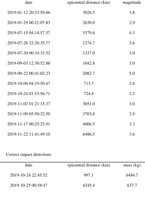
2019-01-12 20:23:50.66 3026.5 3.8 2019-01-29 00:21:07.83 2630.0 2.9 2019-07-15 04:14:57.37 5379.6 4.3 2019-07-20 22:26:35.77 1274.7 3.6 2019-07-30 00:34:15.52 1337.0 3.0 2019-09-03 12:30:52.88 1042.8 3.0 2019-09-22 00:41:02.23 2082.7 5.0 2019-10-06 04:19:50.47 713.7 2.6 2019-10-24 01:53:56.71 724.6 2.5 2019-11-02 01:21:15.37 3051.0 3.0 2019-11-09 05:50:32.50 3703.6 2.9 2019-11-17 00:25:25.91 4006.5 3.3 2019-11-22 11:41:49.10 6486.5 3.6

Correct impact detections

date epicentral distance (km) mass (kg)

2019-10-24 22:45:52 997.1 6484.7

2019-10-25 00:58:47 4245.4 637.7

Table 1. Correct detections from the School Team (Van Driel et al., 2019).

503

504

505

506

(25)

24 List of Figure Captions

508

Figure 1. Map of the School Team. (a) Global view. (b) An enlargement of European Schools.

509

(c) An enlargement of Caribbean Schools (French and Haïtian). White diamonds: location

510

marker.

511

512

Figure 2. The April 7, 2014, Mw 4.9 Barcelonnette ((a) and (b)) and the April 16, 2016, Mw

513

7.8 Ecuadorian region earthquakes ((c) and (d)) recorded at the BLOR educational station

514

(southeastern France, epicentral distances of 0.6° and 87.6° respectively). (a) Upper

515

seismogram: raw vertical component signal (50Hz sampling rate). Lower seismogram: raw

516

signal decimated to 2 Hz. (b) An enlargement of the starting record of the earthquake from (a).

517

Note that the amplitude scale for the decimated signal is ten times smaller than the scale for the

518

raw signal. (c) Upper seismogram: raw vertical component signal (50Hz sampling rate). Lower

519

seismogram: raw signal decimated to 2 Hz. (d) An enlargement of the starting record of the

520

earthquake from (c). SR: sampling rate.

521

522

Figure 3. Synthetic marsquake on January 12, 2019 (vertical component). (a) Raw seismogram.

523

(b) Raw seismogram filtered with bandpass filtering from 0.001 Hz to 0.01 Hz. (c) Raw

524

seismogram filtered with bandpass filtering from 0.01 Hz to 1.0 Hz. (d) Raw seismogram and

525

corresponding spectrogram. (e) An enlargement of the black dashed rectangle in (d). Black

526

dashed ellipse: supposed frequency signature of Rayleigh waves.

527

528

Figure 4. Elements for the epicenter location from Rayleigh waves. a) Scheme of the three

529

surface paths corresponding to the t1, t2, and t3 arrival times in b). Gray star: surface seismic

(26)

25

source. Gray inverted triangle: seismic station. b) Raw synthetic seismogram and corresponding

531

spectrogram on September 22, 2019 (vertical component). This picture comes from a screenshot

532

with SG2K80. LR1, LR2 and LR3: pick of the Rayleigh wave passage at the station. t1, t2, t3:

533

corresponding arrival times.

534

535

Figure 5. Back-azimuth estimation for the event on September 22, 2019. (a) An enlargement of

536

the first P waves on each component, without rotation. (b) New amplitudes computed from a

537

rotation of 65° clockwise. a) and b) are screenshots from SG2K80. E: east component. N: north

538

component. Z: vertical component. (c) Relationships between P wave amplitudes from the three

539

components, azimuth and back-azimuth direction. Azimuth: direction of the first ground motion

540

with 180° ambiguity. Back-azimuth: true direction of the first ground motion determined from

541

the P wave polarity on the vertical component.

542

543

Figure 6. Synthetic seismograms from January 10 to January 15, 2019, compiled by a group of

544

students. Vertical black lines: start of a new terrestrial day. Vertical black dashed lines: start of

545

a new martian sol. Double arrows with black dashed vertical segments: marker of the lag

546

between midnight (UTC) and the start of the middle daily event on January 10, 2019. From

547

January 11 to January 15, students observed that the lag increased day after day. E: East

548

component. N: North component. Z: vertical component.

549

550

Figure 7. Study of the unknown event detected by students on July 15, 2019. Raw seismogram

551

filtered with bandpass values from 0.1 Hz to 1.0 Hz and the corresponding spectrogram.

552

Vertical black lines: pick of Rayleigh waves clearly identified in the spectrogram. Vertical black

553

dashed line: pick of LR3 hypothesized by students.

(27)

26 Figures

555

556

557

Figure 1. Map of the School Team. (a) Global view. (b) An enlargement of European Schools.

558

(c) An enlargement of Caribbean Schools (French and Haitian). White diamonds: location

559 marker. 560 561 562 563 564

(28)

27 565