COQOPERATIVE CONTROL OF TWO ACTIVE
SPACECRAFT DURING PROXIMITY OPERATIONS
by
Robert J. Polutchko
S.B., Massachusetts Institute of Technology, (1985)
SUBMITTED IN PARTIAL FULFILLMENT OF THE REQUIREMENTS FOR THE DEGREE OF
MASTER OF SCIENCE
IN AERONAUTICS AND ASTRONAUTICS AT THE
MASSACHUSETTS INSTITUTE OF TECHNOLOGY AUGUST 1989
© Robert J. Polutchko, 1989
Signature of Author
Deo ent of Aeronautics and Astronautics
August 1, 1989 Certified byProfessor Walter M. Hollister, Thesis Supervisor Professor of Aeronautics and Astronautics Certified by
Edward V. Bergmann, Technical Supervisor
1Charles Stark Draper Laboratory
Accepted by
"- ....--...o.L ld.•Y. Wachman Chairman, Department Graduate Committee Of .
bte
29 1989
Aero
I4
4
COOPERATIVE CONTROL OF TWO ACTIVE SPACECRAFT DURING PROXIMITY OPERATIONS
by
Robert J. Polutchko
Submitted to the Department of Aeronautics and Astronautics on August 1, 1989 in partial fulfillment of the requirements for the degree of Master of Science.
ABSTRACT
A cooperative autopilot is developed for the control of the relative attitude, relative position, and absolute attitude of two maneuvering spacecraft during on orbit proximity operations. The autopilot consists of a open-loop trajectory solver which computes a nine dimensional linearized nominal state trajectory at the beginning of each maneuver and a phase space regulator which maintains the two spacecraft on the nominal trajectory during coast phases of the maneuver. A linear programming algorithm is used to perform jet selection. Simulation tests using a system of two space shuttle vehicles are performed to verify the performance of the cooperative controller and comparisons are made to a traditional "passive target / active pursuit vehicle" approach to proximity operations. The cooperative autopilot is shown to be able to control the two vehicle system when both the would be pursuit vehicle and the target vehicle are not completely controllable in six degrees of freedom. The cooperative controller is also shown to use as much as 37% less fuel and 57% fewer jet firings than a single pursuit vehicle during a simple docking
approach maneuver.
Thesis Supervisor: Title:
Technical Supervisor: Title:
Professor Walter M. Hollister
Professor of Aeronautics and Astronautics, M.I.T
Edward V. Bergmann
Section Chief, Flight Systems Section Charles Stark Draper Laboratory
ACKNOWLEDGEMENTS
I wish to express my gratitude to Prof. Walter Hollister for serving as my thesis advisor and for his constructive advice during the course of this research. I also wish to thank Edward V. Bergmann for being my technical advisor for this thesis and for the valuable recommendations he has provided. I extend thanks to Bruce Persson for the valuable insight he provided during numerous discussions of this cooperative controller design and the proximity operations problem. Many other members of the technical staff at the Charles Stark Draper Laboratory provided technical assistance and support during this research. I am grateful for their help.
I would like to thank the Charles Stark Draper Laboratory for sponsoring this research and for providing a graduate fellowship.
Finally, and most importantly, I wish to thank my family for the invaluable encouragement and support they have provided throughout my education. Any successes I have enjoyed are merely the fruit of their love and understanding.
Publication of this report does not constitute approval by the Charles Stark Draper Laboratory or the Massachusetts Institute of Technology of the findings or conclusions contained herein. It is published only for the exchange and stimulation of ideas.
TABLE OF CONTENTS
CHAPTER 1 INTRODUCTION TO PROXIMITY OPERATIONS ... 6
1.0 Introduction ... ... 1.1 Background ... 7
1.2 Application ... 1.3 Overview of the Cooperative Controller ... 10
1.4 Outline of this Thesis ... ... 12
CHAPTER 2 ROTATIONAL MOTION DURING PROXIMITY OPERATIONS...14
2.0 Introduction ... 14
2.1 Kinematics of a Rigid Body ... ... 14
2.2 Euler's Moment Equation ... 18
2.3 Attitude Displacements ... ...22
2.4 Relative Rotational Motion of Two Spacecraft...24
CHAPTER 3 SPACECRAFT TRANSLATION DYNAMICS ... 25
3.0 Introduction ... 25
3.1 Translational Motion of a Rigid Body ... 25
3.2 Two Body Problem ... ... ...27
3.3 Translational Motion with Respect to a Nominal Circular Orbit ... 28
3.4 Relative Translational Motion of Two Active Spacecraft ... 35
CHAPTER 4 JET SELECTION FOR COOPERATIVE CONTROL ... 37
4.0 Introduction ... ...37
4.1 The Two Vehicle Jet Selection Problem ... ...37
4.2 Linear Programming ... 42
4.3 The Revised Simplex Algorithm ... 46
4.4 Implementation of the Revised Simplex Jet Selection Algorithm ... 52
CHAPTER 5 TWO VEHICLE TRAJECTORY SOLVER ... 59
5.0 Introduction ... 59
5.1 Final State Equations...60
5.2 Trajectory Solution Algorithm ... 65
CHAPTER 6 PHASE SPACE REGULATOR ... 77
6.0 Introduction...77
6.1 Velocity to be Gained... ... 77
6.2 Phase Sphere ... 79
6.3 Phase Space Control Law... ... 81
6.4 The Cooperative Control Phase Space Regulator .. ... 87
CHAPTER 7 PERFORMANCE VERIFICATION TESTS ... ... 89
7.1 The Test Environment... 89
7.2 Long Maneuver Test... ... 90
7.2.1 Cooperative Control During a Long Maneuver ... 90
7.2.2 Non - Cooperative Maneuver ... 100
7.3 Jet Failure Test ... ... ... ... .103
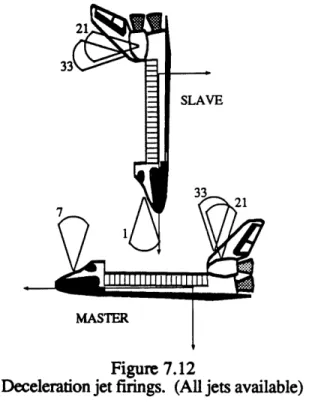
7.3.1 All Jets Available ... 105
7.3.2 Slave Shuttle's Forward Jets Unavailable ... 112
7.3.3 Slave's Forward Jets & Master's +Z Jets Unavailable ... 119
7.3.4 Slave's Forward Jets & Master's Primary Jets Unavailable ... 125
7.3.5 Summary of Jet Failure Tests ... ... ... 126
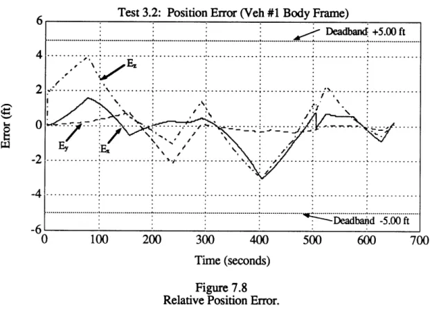
7.4 V-Bar Approach Test... 127
7.4.1 Master Vehicle Jets Unavailable ... 129
7.4.2 All Jets Available ... 131
7.4.3 Master Vehicle More Efficient Than Slave Vehicle ... 134
7.4.4 Upward Firing Jets Less Efficient... 136
7.4.5 Summary of V-bar Tests ... ... .... 137
CHAPTER 8 SUMMARY AND CONCLUSIONS... 142
8.0 Conclusions ... .142
8.1 Contributions... 143
8.2 Recommendations for Additional Work... 144
CHAPTER 1
INTRODUCTION TO PROXIMITY OPERATIONS
1.0 Introduction
As the frequency and complexity of space missions increase, the scope of the tasks to be performed on orbit will grow beyond the capabilities of single spacecraft and will necessitate collaboration among multiple specialized vehicles. The safe and efficient operation of multiple spacecraft in close proximity to one another will place new demands on both pilots and flight control systems in the near future. Inflight construction of the space station and other complex on orbit tasks will require a flexibility and spontaneity beyond current proximity operation techniques. Operations between the space station, orbital maneuvering vehicles, free flyers, and the shuttle will continue to depend on the ability to routinely perform complex rendezvous, formationkeeping, and docking maneuvers.10 Though shuttle crews can perform many of these tasks manually, extended duration formationkeeping requirements and the introduction of highly maneuverable unmanned vehicles will cause crew workloads to increase and will necessitate the development of automatic systems to handle standard proximity operations.
The proximity operations problem has usually been solved using an 'active' pursuit spacecraft to establish a desired position and attitude relative to a 'passive' target vehicle.12 This pursuit vehicle approach neglects both the ability of the 'passive' vehicle to perform complementary attitude and translation maneuvers and the superior fault tolerance of a system employing two active vehicles. Consequently, the pursuit vehicle maneuver sequences are less efficient and more constrained than those generated using the control authority available from both vehicles.
This paper presents a cooperative autopilot approach to the control of joint maneuvers of two spacecraft during proximity operations. The cooperative approach considers the two spacecraft as a single system and exploits the rotational and translational capabilities of each spacecraft in order to control the state of this system. The efficiency and robustness to jet failures of this new autopilot design is demonstrated.
1.1 Background
Previous treatments of spacecraft proximity operations have focussed on the control of the motion of a single maneuvering vehicle in a reference frame fixed to a target vehicle.18,2 1,22 This pursuit vehicle initiates rendezvous and docking, performs formationkeeping activities, and implements collision avoidance maneuvers. Though the target vehicle may perform some independent attitude control during the approach phases of the rendezvous, the commanded attitude of the target vehicle is pre-determined and is not updated to account for the actual state of the pursuit vehicle. The closed-loop control used in this approach to proximity operations formulates reaction control jet firing commands for the pursuit vehicle in order to minimize the fuel consumed, the time to reach the target state, and/or the final state error.
Single vehicle control was successfully applied to terminal phase proximity operations and docking during the Apollo and Skylab missions. On these missions the target spacecraft remained essentially passive while the pursuit vehicle performed simple, manually controlled approach maneuvers. During the shuttle era, the target spacecraft have been science platforms or communication and observation satellites which have not been designed for extensive orbital maneuvering. Consequently the space shuttle performs most of the proximity operations maneuvers even though it is more massive than most of its rendezvous partners. The use of single vehicle control avoids the complexity of the cooperative maneuvering problem and in current space shuttle operations does not significantly impact the performance of the two vehicle system due to the imbalance of control authority between the vehicles.
The introduction of the next generation of advanced spacecraft will add a new dimension to proximity operations. Spacecraft like the Orbital Maneuvering Vehicle (OMV) will be unmanned, maneuverable, and designed specifically for the rendezvous mission. Future enhancements to the shuttle autopilot will make the shuttle a more agile and more efficient proximity operations vehicle. Artificially constraining one of these advanced vehicles to remain passive during proximity operations eliminates the natural synergism that exists between two agile spacecraft. Conversely, employing the control authority of both spacecraft to perform coordinated maneuvers will provide an increased level of flexibility and a greater margin of safety during proximity operations.
In many mission scenarios spacecraft will be required to operate at a range of only a few vehicle lengths. Control of the relative attitude and position of two spacecraft in this
operating regime is especially difficult due to stringent plume impingement constraints and "fail-safe" collision avoidance rules.14
Many spacecraft rely on hot gas reaction control jets to perform on orbit maneuvers. The space shuttle reaction control system utilizes bipropellent (nitrogen tetraoxide and monomethyl hydrazine) hypergolic jets.4 These jets expel a plume of high velocity gas when fired that could damage or disrupt a neighboring vehicle during close proximity operations. While vehicles with delicate optical instruments or solar panels are particularly sensitive to the chemical effects of the jet plume, spacecraft with flexible or articulated appendages may experience adverse perturbations due to the force of the plume impingement. Vehicles operating in close proximity to the space station will be required to orchestrate maneuvers such that the thruster exhaust does not impinge on the station.10
When operating in close proximity to a spacecraft which is sensitive to jet plume effects, the space shuttle crew manually disallows jet firings which may impinge upon the target spacecraft. For example, if the shuttle passes beneath such a vehicle all upwardly firing jets are disallowed.14 In each situation where a jet or set of jets is to be disallowed the controllability of the maneuvering vehicle must be re-evaluated. During single active vehicle proximity operations, the pursuit vehicle must be capable of avoiding a collision with the passive target vehicle under a variety of limited failure modes. The types of maneuvers a pursuit vehicle may perform become extremely limited under collision avoidance and plume impingement constraints as the spacecraft get very close. If a large number of jets on the pursuit vehicle are deselected or have failed, the maneuvers available to the crew will probably be fairly fuel inefficient and in the extreme case, the pursuit vehicle may become unable to control the relative states of the two vehicles.
The cooperative control scheme developed in this thesis exploits the natural redundancy provided by the actuators on the target vehicle in order to make the two vehicle
system more robust to jet unavailabilities.
1.2 Application
The cooperative autopilot approach to the control of two vehicle proximity operations is applicable to any two spacecraft. This thesis develops the concept for a system of two shuttle vehicles. As the principle support vehicle for construction of the
space station, deployment and retrieval of advanced spacecraft, and other maintenance and resupply operations, the shuttle will continue to conduct rendezvous missions well into the next century. In addition, the shuttle's asymmetrical mass distribution and complicated configuration of forty-four reaction control jets make it a fine example of a general class of complex, highly maneuverable spacecraft. Two identical spacecraft are employed to ensure that the difference in performance between the standard single vehicle control architecture and the new cooperative control architecture is not a consequence of introducing a more efficient or otherwise superior spacecraft in place of the non-maneuvering target vehicle. Specifically, the use of two shuttle vehicles will facilitate direct comparisons between cooperative control and traditional 'shuttle as a pursuit vehicle' proximity operations solutions.
The general scenario to be considered in this thesis is a joint maneuver by two space shuttles operating in low earth orbit (LEO). The shuttles are in nearly identical 90 min (300 nm) circular orbits at a relative range of less than 3000 ft. The maneuver will typically last less than one orbit. The initial attitude of each vehicle is unconstrained. The two spacecraft are idealized as three dimensional rigid bodies; the mass (m), inertia (I), and center of mass location (ran), of each vehicle is constant and known in the vehicle's body fixed coordinate frame. Similarly, the locations (rj), and the thrust vectors (fj), of the 44 reaction control jets on each orbiter are known in the body fixed frames. The attitude and position of each vehicle in an earth centered inertial coordinate frame is available from onboard navigation devices. The relative states of the vehicles are assumed to be available either as a direct measurement (by a laser ranger for instance) or as the difference of the inertial states. These sensor and estimator requirements are not unique to a cooperative control architecture and have already been proposed for use during traditional proximity operations.22
The cooperative autopilot resides on the 'master' vehicle; the other vehicle is designated the 'slave'. A communication link similar to those proposed for use by remotely piloted spacecraft such as the OMV is assumed to exist between the two spacecraft. The slave vehicle provides mass property parameters, jet status data as well as current position and attitude information to the master vehicle. The master vehicle passes the numbers of the jets to be fired and the corresponding firing times to the slave vehicle.
1.3
Overview of the Cooperative Controller
The cooperative controller is a two tiered system consisting of an open-loop maneuver planner block and a closed-loop regulator block. The maneuver planner employs a linearized model of the vehicles to plan an open-loop trajectory consisting of an acceleration burn, a coast period, and a deceleration burn. During the coast phase of the maneuver the regulator monitors the state errors and computes any necessary corrective jet firings in order to keep the system following the pre-planned trajectory. Figure 1.1 is a block diagram of the cooperative controller.
The trajectory solver (chapter 5) accepts a state command form a guidance algorithm or pilot interface module and computes a trajectory consisting of an acceleration burn, a coast, and a deceleration burn which carries the system from the current state to the commanded final state. The acceleration and deceleration jet firing commands are determined by a simplex jet selection algorithm (chapter 4) which minimizes a cost function based on total jet firing time. The trajectory itself is optimized to minimize the final state error.
Once a satisfactory trajectory has been determined the trajectory solver passes the acceleration jet firing commands, the desired value of the system state at the beginning of the coast phase of the trajectory, and the deceleration jet firing commands to the trajectory sequencer. The trajectory sequencer initiates the planned maneuver by passing the jet firing commands to the jet sequencer which actually implements them. At the end of the acceleration burn the trajectory sequencer initializes the nominal trajectory state generator (section 5.3) with the pre-computed value of the system state at the beginning of the coast phase and activates the phase space regulator (chapter 6).
During the coast phase of the maneuver the nominal trajectory generator updates the target value of the system state at 12.5 hz using a linearized model of the two vehicle system. The state error is then computed as the difference between the current state and the target state. The phase space regulator compares the state error to a set of predetermined thresholds and determines when a corrective jet firing is required. To implement a corrective jet firing a velocity impulse request is passed to the simplex jet selection
algorithm which computes an optimum set of jet firing commands. These feedback initiated jet firing commands are immediately passed to the jet sequencer and implemented.
0 o 6obb °•,• - : Qo O o U
I
$I
L
r32I
-14
At the end of the coast phase of the maneuver the pre-computed deceleration jet firings are implemented. At the end of the deceleration jet firing sequence the two bum maneuver is complete. A new maneuver is then commanded or the coast phase feedback loop is reactivated to maintain the two vehicle system at the commanded state. In the latter case the output of the trajectory state generator is the commanded state and is constant.
1.4 Outline of this Thesis
Chapter 2 develops the rotational equations of motion for a body in space and derives an expression for the relative motion of two rigid bodies.
Chapter 3 presents a derivation of the Clohessy - Wiltshire equations for the translational motion of a body with respect to a neighboring circular orbit. These equations are then used to develop an expression for the relative motion of two maneuvering spacecraft.
Chapter 4 develops the cooperative control jet selection algorithm. The two vehicle jet selection problem is first formulated as a linear programming problem. The properties of linear programming problems are then presented and the revised simplex algorithm introduced as a solution technique. Finally the practical aspects of the application of the revised simplex algorithm to the jet selection problem are discussed.
Chapter 5 develops the two vehicle trajectory solver which determines the open-loop trajectory for the two burn maneuver. First, the linearized algebraic equations describing the final state of the system in terms of the initial state and the coast velocity parameters are derived. An iterative method for determining the values of the coast velocity parameters which minimize the final state error is then presented. The coast phase nominal state trajectory generator is formulated.
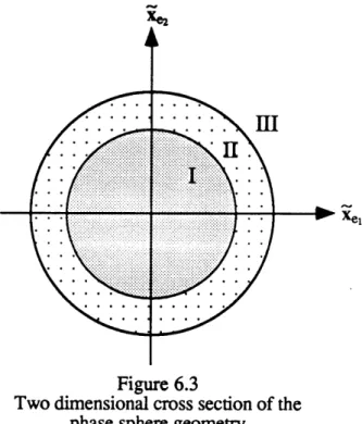
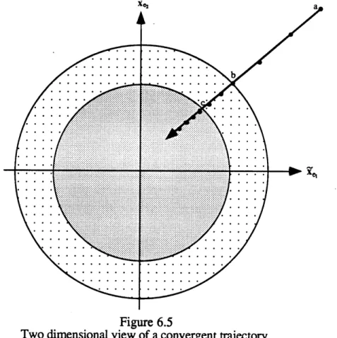
Chapter 6 formulates the phase space regulator for the two spacecraft cooperative control problem. The velocity to be gained algorithm and the concept of the phase sphere are introduced as the basis for general phase space control. The application of phase space control to the cooperative control problem is then discussed.
Chapter 7 contains a description of the tests used to verify the operation of the cooperative controller for the two space shuttle example. A detailed analysis of the results of the tests is presented and comparisons are made between the pursuit vehicle approach and the cooperative control approach to proximity operations.
Chapter 8 contains a summary of this investigation and outlines some key areas for further research which should be addressed prior to an actual flight test of this system.
CHAPTER 2
ROTATIONAL MOTION DURING PROXIMITY
OPERATIONS
2.0
Introduction
The rotational motion of a spacecraft is based primarily on rigid body angular momentum principles. This section provides a derivation of Euler's Momentum Equations. Though a general closed form solution of Euler's equations does not exist, in certain cases good approximations may be made and accurate solutions formulated. The essential approximations to be employed during the development of the cooperative autopilot are introduced and the linearized rotational equations of motion formulated. Quaternions will be employed to express the angular displacements between reference frames and are briefly introduced.
2.1 Kinematics of a Rigid Body 7,8
Consider a rigid body of mass m as a collection of particles with individual mass mi (figure 2.1). The ith particle has instantaneous position Ri and instantaneous velocity Ri with respect to an inertial reference frame. The linear momentum of this particle is given by Newton's Second Law:
Pi = mi Ri (2-1)
The moment of this momentum about an arbitrary point O located at Ro is defined as
hoi = ri x mi Ri (2-2)
where ri is the instantaneous position of the ith particle with respect to an intermediate
coordinate frame centered at the point O. Since Ri = Ro + ri , the first derivative of Ri is Ri = Ro + ii and the moment of momentum becomes
Figure 2.1
Position of particle mi in an inertial and a rotating reference frame.
The first term in this expression is the angular momentum of the particle observed in the intermediate coordinate frame and the second term is the correction due to the motion of the point O.
The total angular momentum of the body about point O is the vector sum of the angular momenta of the i particles.
Ho= = rixmiii - Rx Xrimi (2-4)
i i i
If the point O is constrained to correspond to the center of mass of the rigid body, then by definition
ri mi = 0 (2-5)
and the angular momentum equation becomes
Ho = X ri x miii (2-6)
The time derivative of the position of the ith particle in the intermediate frame with respect to the inertial reference frame is
ii = r. + x ri (2-7)
where rr indicates differentiation of ri with respect to time in the intermediate coordinate frame and ao is the angular velocity of the body with respect to the inertial frame. Since the body is rigid and the intermediate reference frame is fixed in the body, r0 = 0 and
ii = ax ri (2-8)
Substituting this expression into the expression for Ho yields
Ho = ri x x mi(c x ri) (2-9)
As the number of particles in the body is allowed to increase while the individual mi
decrease such that m
=
I mi remains constant, the particle model of the body approaches a
continuum model. In the limit, this summation over the particle mass elements becomes an
integration over the differential elements of mass, dm.
H. = r x (o x r) dm (2-10)
The argument of this integral is evaluated by expressing the vector products in component
form along the body fixed coordinate directions.
rx (cox r) = ( cox (y2+Z2) - oy (xy)
-Oz (xz)) 1
+
(-ox
(xy) + coy (x2+z2) - (y)) (2-11)+
(
-o (xz) - Oy (yz) + o (x2+y2))i
The components of the angular momentum along the body axes are then
Hx=
cxf
(y
2+z
2) dm
-
y
(xy) dm
-
zf(xz) dm
HY = -x (xy) dm +
cyJ
(x2+Z2) dm - (yz) dm (2-12)Hz
=
-oxf
(xz) dm
-
yJ
(yz) dm
+
oJ
(x
2
+y
2
) dm
The integrals in the above equations are constant in any coordinate frame fixed to the rigid
S
(y
2 2)
dm
=(x
2 2) d
=f
(x
2+y
2) dm
(2-13)
are defined as the moments of inertia and
=xy=
f(xy)
dm
Ixz
=f
(xz) dm
Iz =
f
(yz) dm
(2-14)
as the products of inertia. The components of the angular momentum may be rewritten in terms of these constants.Hx = Ixxtox - Ixyoy - Ixzoz
Hy =- IxyOx + IyyOy - IyzOz (2-15) Hz = -Ixzox
-IyztOy + IzztOz
Matrix notation is often the most convenient way to write an expression for the total angular momentum.
Ho = I (2-16)
The matrix I is the inertia tensor
[Ixx
-Ixy IxzI =
-
Ixy Iyy -Iyz (2-17)l-Ixz -yz Izz
The rate of change of the angular momentum is calculated by taking the derivative of this last expression for Ho with respect to time.
Ho = 1i + I, = I*' + oxIo + Io* + I (ox o) (2-18)
Here I* and o'* are the derivatives of I and co in the body fixed reference frame. Since the inertia tensor of a rigid body is constant in a frame fixed in the body, I* = 0 and hence the first term on the right hand side of this equation is zero. Since (o x o = 0, the last term on the right is also zero. The rate of change of the angular momentum is then expressed
2.2 Euler's Moment Equation
7,8
Newton's second law relates the force on a particle, Fi, to the linear momentum of the particle, pi.
(2-20) where
Pi - mi Ri (2-21)
Since the mass of a particle is constant, Newton's second law may be written
Fi = mi Ri (2-22)
From equation 2-6, the total angular momentum of the body can be written in terms of the of the momenta of the individual particles
Ho = ri x miri (2-23)
Differentiating this expression for the angular momentum with respect to time and noting
that i'i x ri = 0
Ho
= X ri x miji (2-24) Since ri = Ri - RoHo
= X ri x miRi i + 0 x miri iThe origin of the body coordinate frame has been constrained to be the center of mass of the rigid body. Thus by definition of the center of mass
Smiri = 0 (2-26)
and the rate of change of the angular momentum is
Ho
=
ri xmiRki
(2-25)
The factor miki is the time rate of change of the linear momentum of the it h particle and
may be replaced using the above expression for Newton's second law
Ho = ri x Fi (2-28)
i
If the external force on the ith particle is defined as Ei and the force exerted on the
ith particle by the jth particle is defined as fij, then the total force exerted on the ith
particle is
Fi = Ei + C fij (2-29)
Substituting this expression for the total force into equation 2-28
Ho = X ri x Ei + X ri x fij (2-30)
i i j
The double summation in this equation is composed of pairs of terms of the form
(ri x fij) + (r x fji)
(2-31)
From Newton's third law
fij = -fji (2-32)
so that the double sum may be rewritten
, ( ri - rj )x fij (2-33)
i j
In an ideal rigid body, ( no particle deformation ), the mutual forces between particles act through the particle centers. Consequently, the direction of the fij force vectors correspond with the direction of the the relative position vectors ( ri -rj ) and each cross product in the double summation is zero. The rate of change of the angular momentum vector of a rigid body is
Ho = ri x Ei (2-34)
Ei is the total external force vector applied to the ith particle. The corresponding moment
applied to the rigid body by this force is given by
. and the total external moment applied to the rigid body is
Mo = ri xEi (2-36)
Finally, combining equation 2-34 and 2-36 we arrive at the familiar governing equation for the rotational motion of a rigid body
IHo
= Mo (2-37)When the total external moment applied to the body is zero, this equation is merely
a statement of the principle of the conservation of angular momentum. In addition, if the kinematic expression for the rate of change of the angular momentum (equation 2-19) is substituted for Ho , this equation becomes
Mo = Io + CxI (2-38)
This is the matrix form of Euler's Moment Equations. These three coupled, non-linear differential equations completely describe the rotational motion of a rigid body about its center of mass. Though a general closed form solution of Euler's equations does not exist, in special cases when the body is axisymmetrical, the angular velocity is small, or the applied moments are large, good approximations can be made and simple closed form solutions to the resulting linear differential equations derived.
Euler's equations may be written in component form as
Mx = (IxxO - IxyOy - IxzOz)
-
IxzCOxOy
-
IyzCo + Izz"OZ)
+ IxyOxOz - IyyOyO)z + IyzO)2
My= (- Ixyx + Iyyy - IyzOz)
+ Ixx,)xOz - IxyOyOz - IxzCJ)Z (2-39)
Mz - (- IxzO)x -
lyz(Oy
+ IzzOz)- IxyO + Iyy(O)xO)y - Ixz()xOz
-
IxxCOXOY
+
Iy
+
IxzOyCOz
If the angular rates ox, oy, these equations reduced to
oz are small, the second order terms may be neglected and
Mx = IxxOx -
Ixycy
-My = - IxyC x + IyyOy - IyzOjz (2-40)
Mz =
Ixz - Iyzy- y+
IzziWhich may be re-written in matrix form as
M= Ic (2-41)
so that the rate of change of the angular velocity is
(2-42)
If in addition, the external moment applied to the equations of motion become
co = constant
vehicle is zero, then the spacecraft
(2-43)
Many spacecraft employ reaction control jets to perform attitude and position control. Each reaction control jet on a spacecraft is described by its location (rj) and its force vector (fj). The moment applied about the spacecraft center of mass (rcm) by the jth jet is
Mj = (rj -rn) X fj (2-44)
Define aj, the angular acceleration due to the jth jet, as
If a control vector u is defined such that
UJ1 when the jth jet is firing
Uj 0 otherwise (2-46)
then the equation 2-42 governing the rotational motion of the spacecraft may be written
N
i
=aj
uj
j=1
(2-47)
where N is the number of reaction control jets on the spacecraft.
2.3 Attitude Displacements 17,20
Consider a coordinate frame rotating with a constant angular velocity co with respect to a reference coordinate frame. The angular velocity vector may be written as
o
=
Ii
=
d~-
xi+
m i,
+ n
z)
(2-48)Integrating this constant angular velocity over the period At = tl - to
ti t1
Scodt
= adO
I
(2-49)This angular displacement vector represents a rotation by an angle AO = d (At) about an axis i~. A more convenient representation of this rotation is Hamilton's four element quaternion.
q
a
q _ = (2-50)
8, a, 03, y are the Euler Parameters and are defined as
dO At) i dt
8 = cos ~AO
2 a = sin 1AO
2
S= m sinlAO2From this definition it is clear that
q = aix + + ylz = (sin
2A
0)and that
a
2+ 0+ 2+
2
1
(2-52)
(2-53)
The new orientation of a reference frame following a rotational displacement 0 about an axis i is given by
qf = qo qe (2-54)
where qo is the quaternion representation of the original orientation of the reference frame and quaternion multiplication is defined by
ql q2 = 812 - qTq2 + 12+ &2q1 + q1X q2 -a1 -01 a 581 71 61 'Y1 -1 X1 561 82 a2 02 7Y2 -(2-55) = S(ql) q2
A vector may be rotated thru an angle represented by the quaternion q in the
following manner. Define the four element vector io as
(2-56)
then the rotated vector is
r=q ro q (2-57)
y = n sin -AO2 (2-51)
i
-al
2.4 Relative Rotational Motion of Two Spacecraft
Consider the rotational motion of two rigid spacecraft. Define the relative angular velocity as
OR = 02 - 01 (2-58)
where co and w2 are the angular velocity of vehicle #1 and vehicle #2. The rate of change
of the relative angular velocity is the derivative of this equation in an inertial reference frame
(WR = 6)2 - (1 (2-59)
Euler's Moment equation provides an expression for the angular acceleration experienced by each vehicle in terms of the external moment applied to the vehicle. Thus wR may be re-written
(OR =
1
2-1(M2 - 02 X 2 0)2) - I1-1(M - (01 X 11 (01) (2-60)As before, if the angular velocity of each vehicle is small, the second order rate terms may be neglected. Since the external moments experienced by each spacecraft are primarily due to reaction control jet activity, the moments M1 and M2 may be expanded as the sum of the
moments applied by the individual jets.
N2 /N
R = 2-1 (r2j -r2m) x f2
j
- I•(rij
-rlcm) Xflj(2-61)
j=1
1(2-61)
The additional subscript has been added in this expression to indicate the vehicle referenced. As before, if the angular acceleration of the spacecraft due to firing the jth jet is aj the this equation may be re-written as
WR =c2 j u2j -j 1j j) (26u
=l \j=1 l (2-62)
where ul, u2 are the control vectors for the two vehicles. When none of the jets in the two vehicle system are active, the angular momentum of the system is conserved and the governing equation for the relative attitude of the vehicles becomes
CHAPTER 3
SPACECRAFT TRANSLATION DYNAMICS
3.0 Introduction
The translational motion of a spacecraft is based upon the linear momentum of an equivalent mass particle under the influence of external forces. This section derives the equations of motion for a rigid body undergoing pure translation. The predominant external force on a spacecraft is the gravitational force of the planet it is orbiting. A formulation of the general two-body problem is presented. Though a treatment of the methods generally employed to solve the resulting non-linear second order differential equations is beyond the scope of this thesis, these equations serve as the basis of a derivation of the Clohessy - Wiltshire18 (Euler-Hill) equations for motion relative to reference point travelling in an unperturbed circular orbit. The primary interest of this thesis is the control of the relative motion of two active spacecraft. The equations of relative motion are derived in a "local vertical local horizontal" reference frame.
3.1 Translational Motion of a Rigid Body 7
Consider a rigid body of mass m as a collection of particles with individual mass mi. The ith particle has an instantaneous position Ri and instantaneous velocity Ri with respect to an inertial reference frame. The linear momentum of this particle is defined as
Pi = mi Rki (3-1)
Define ri as the instantaneous position of the ith particle with respect to an intermediate
coordinate frame centered at the point O such that Ri = Ro + ri , where Ro is the
instantaneous position of the point O in the inertial frame. The linear momentum of the ith particle is then
Pi = miRo + miii (3-2)
P = mikR + miii (3-3)
i i
Since the mass of the ith particle is constant,
i miii = (i miri (3-4)
If the point O is constrained to correspond to the center of mass of the rigid body, then by definition
ri mi = 0 (3-5)
and the linear momentum equation becomes
p = XmiRo = Ro mi (3-6)
i i
By definition m = C mi so that the total linear momentum of a rigid body reduces to i
p = m]k (3-7)
which is just the linear momentum of a point mass m located at the center of mass of the body. The rate of change of the total linear momentum is the derivative of this expression with respect to time
=
mR
0(3-8)
If the external force on the ith particle is defined as Ei and the force exerted on the ith particle by the jth particle is defined as fij, then the total force exerted on the ith particle is
Fi = Ei + fij (3-9)
The total force on the body is the sum of the total force acting on each particle
F = Fi = Ei+ fij (3-10)
i i i j
From Newton's third law it is clear that
and thus that the double summation over the internal force vectors in the total force expression is zero. The total force is then the sum of the external forces applied to the particles in the body.
F = Ei (3-12)
Applying Newton's second law (Fi = pi) permits p to be eliminated between
equation 3-8 and equation 3-12 and yields the governing equation for translational motion of a rigid body.
m -= Ei (3-13)
As expected, the pure tanslational motion of a rigid body in the presence of external forces is equivalent to the motion of a single particle of equivalent mass located at the center of mass of the body translating under the influence of a single force equivalent to the vector sum of all the external forces.
3.2 Two Body Problem 17
Consider two bodies with instantaneous positions R1 and R2 with respect to an
inertial reference frame. If the bodies are far enough apart, of have sufficiently spherical mass distributions and are not in contact with each other, then their mutual gravitational attraction will act through their mass centers and they may be treated as particle masses ml and m2. Newton's law of gravitation states that any two particles attract one another with a force of magnitude
F - Gm1m2
2 (3-14)
R12
acting along the line joining them. Here G is the universal gravitational constant and R12 is
the distance between the particles.
R12 = R21 = V(R2
- R1)T(R2 -R1) (3-15)
S=
Gm(R2 - R) F2 = Gmlm (RI - R2)
R321 (3-16)
Newton's second law states
F = mk
(3-17)and may be applied to the gravitational force equation for each vehicle to yield two differential equations describing the motion of the two bodies in the inertial reference frame.
S= Gm2(R2- RI)
R312 R2 = R321 (RI - R2) (3-18)
The motion of m2 relative to ml is obtained by differencing these equations
(2 - 1) = -G(ml + m2) (R2 -R1)
R321 (3-19)
Thus the basic differential equations of relative motion for the two body system is
R+ R R=O
R3 (3-20)
where 9. = G(ml + m2).
In this thesis, the primary interest is the motion of a rigid body about the earth. In this case, the center of mass of the two body system very nearly corresponds with the center of mass of the earth. Thus the relative motion differential equations (3-20) may be interpreted as a description of the motion of a rigid body about a center of attraction.
3.3 Translational Motion with Respect to a Nominal Circular Orbit 18, 7, 11
Consider a reference point travelling in an unperturbed circular orbit about the earth. The motion of the point in an earth centered inertial reference frame is given by
Io + L Ro = 0
Define a "local vertical -local horizontal" reference frame centered on and moving with this reference point. The LVLH unit vectors are defined as:
iz Ro R 7- iy y = Ro xRo = 3-22
- x = iy Xiz (3-22)l
In other terms, iz is defined opposite the instantaneous orbital radius vector, iy is defined opposite the angular momentum vector of the orbit, and ix is defined to complete the right handed coordinate system.
Consider a spacecraft travelling in a separate orbit and experiencing an external perturbation force such as drag from the upper atmosphere, gravitational anomalies, or reaction control jet activity. The motion of this vehicle in an earth centered inertial reference frame is governed by
I1 + R =
1 = a (3-23)
R3
where al is the force per unit mass of the perturbation force. The motion of the spacecraft relative to the reference point is described by the difference of the second order equations
describing the individual motions in inertial space.
i = (1- ) =
R- _ R3 + a (3-24)
Here rl is defined as the instantaneous position of the spacecraft relative to the reference point O.
The position of the reference point, Ro, and the relative position vector, rl, are easily expressed in the LVLH coordinate frame as
Ro = [ 0 -RoIT (3-25)
rl = [x y z ]T (3-26)
Since R1 = Ro + rl, the inertial position of the spacecraft may also be expressed in the
LVLH coordinate frame
The ratio
- (lT RoP" (n RTRI)
R (
(R
R 1 (3-28)may be expressed in terms of the LVLH coordinate variables by substituting the expression in equation 3-25 for Ro and the expression in equation 3-27 for R1.
= R3 (x2 + y2 + (z - Ro)2)-3/2
-29)
R3 (3-29)
During proximity operations rl << Ro and therefore x, y, z << Ro. Under this condition, the second factor in equation 3-29 may be expanded as a binomial series and the equation re-written as
SR (Ro - )-3 R -5(x2 + y2) + H.O.T. (3-30)
Expanding the (Ro-z) terms as binomial series and collecting similar terms yields
= 1 + 3
(x2 + y2)
+ 5 + H.O.T. (3-31)
Since -x_ Y _ << 1 second order terms involving these ratios are neglected leaving
Ro Ro Ro
R3 = 1 + 3 (3-32)
Substituting this expression into equation 3-24
r= (Ro -(1 + 3 R) + al (3-33)
and noting again that R1 = Ro + r
i= R - 3-R - 3 -r,) + a1 (3-34)
R3
Ro
Ro
z
Since RO << 1, the last term in the brackets represents a small fraction of the LVLH coordinate displacements and may be neglected without introducing significant errors.
With these simplifications the linearized differential equation governing the motion of a spacecraft relative to a unperturbed reference orbit becomes
-xJ
ji
=
~
-yi
+
al
(3-35)
2zI
The complete derivative of the position of the spacecraft relative to the orbiting reference point may be written as
ri = r, + co x r (3-36)
where ri is the derivative with respect to the LVLH coordinate system and o is the angular velocity of the LVLH frame relative to the earth centered inertial frame. The complete derivative of this relative velocity is the relative acceleration.
ii
= rI + 2( X r) + 6x r1 + Wx ()x rl) (3-37)Since the LVLH coordinate frame is aligned with the instantaneous radius vector of the reference orbit, the angular velocity of the LVLH frame is equal to the instantaneous angular velocity of the reference point about the center of the earth. For a general unperturbed reference, this angular velocity is time varying and equal to
o = h = _ (3-38)
dt R
where h is the massless angular momentum of the orbit.
When the reference orbit is defined to be an unperturbed circular orbit, Ro is a constant and equal to the semi-major axis of the orbit. From Kepler's Second Law (equal areas in equal time) the angular velocity of the circular orbit is constant and equal to the mean motion of the orbit
CO= h = -Ioly (3-39
Here rlo is the mean motion and iy is the cross-plane unit vector of the LVLH frame. Thus
for a circular reference orbit the complete derivative of the relative position vector may be written
x1 -zi xI
y **
0
2112 0
(3-40)
ri = + 2 0]0 - 2120
Eliminating
ii
between this kinematic expression and equation 3-35 yields the set of three
second order linear differential equations for the relative motion of a spacecraft in the
LVLH reference frame.
Xl = 2Tlo z1 + ax
Y**= - Tloyl+
ay (3-41)
z* = - 210 x + 3lozl + az
These equations are known as the Clohessy - Wiltshire (Euler -Hill) equations and are
often expressed is state space form (X = A X + B f ) as
0 0 0 1 0 0 0 0 0 0 1 0 0 0 0 0 0 1
o
0 0 0 0 210
-192 0 0 0 00
03r1
2-2rn
0
0
xl Yi Z1 0 0 000
0
fx
+ 0 0 0 fy (3-42) mi'0
0
f'
0 mi1 0 S0 0 mi' - _ .1 _g-j twhere al has been replaced by mi'f.
The character of the motion of an unpowered satellite may be ascertained by inspection of equations 3-41 or equation 3-42. The motion of the satellite in the direction perpendicular to the orbital plane (iy ) is uncoupled from the motion along the other LVLH directions and is a simple harmonic oscillation with a period equal to the orbital period of the reference point, 2. Qualitatively, this motion is the consequence of a slight difference in the inclination of the spacecraft and reference orbits.
The motion along the x and z axes is a coupled oscillation. Note however, that when the vehicle is positioned on the LVLH x axis (zi = 0) with zero inplane velocity
(O1, ii = 0) the second derivatives of x and z are also zero and the vehicle is at an
Yl xl
x1
equilibrium point. Consequently, positions along the x axis are efficient points at which to stationkeep and are commonly exploited during many types of proximity maneuvers.
The complete solution of the Clohessy-Wiltshire (C.W.) equations is the sum of their homogeneous and particular solutions. Equations 3-41 may be written as a set of unforced differential equations
x=
2r7ioS=
_- i2 y (3-43)z = -210 i + 3"12 z
For simplicity the subscript 1 has been dropped and the '*' replaced with '' though the
derivative is still to be carried out in the LVLH frame. As noted above, the second equation represents a simple harmonic oscillation and thus the equation governing the motion in the cross-plane direction is
y = yo cos lot + - sin riot
r10
(3-44)
with first derivative
S= •o cos 10t - yo T0 sin rlot (3-45)
Yo and 'o are respectively the initial out-of-plane position and the initial out-of-plane velocity.
To solve the remaining two coupled differential equations describing the in plane motion, integrate the first equation and evaluate the resulting integration constant at the initial condition (tO-0, x=xo, z=zo, etc.)
i = 2TIo0 + (io - 2To zo) (3-46)
Substitute this expression for x into the third equation and collect common terms.
.= - 12 z + (4112 zo - 200io) (3-47)
The solution to this equation will take the form z = Acos7it + BsinTrt + C, where A, B, and C are constants to be determined from initial conditions. The solution is
z = 2io 3zo cos 7ot +
\11
0
(3-48)and has first derivative
z
= zo cos riot - (2o - 3iozo) sin riot (3-49)Substitution of this expression for z into the above equation for 3 yields
= (40 - 6blozo) cos rit + 2iosin olt + (6TIzo - 3io) (3-50)
Since each of the coefficients in this equation is constant, the governing equation for x may be obtained by direct integration. The resulting integration constant is again evaluated at the initial condition, t = 0.
x _ 40 - 6zo sin lot 2'o cos rot + (6iozo - 3o) t + xo + 2ýo
1o
0o
Unlike the other equations, this equation contains the secular term (6ilozo - 3io) t. This term drives the spacecraft in the positive x direction if zo > 0 (spacecraft is below the
reference point) and in the negative x direction if zo < 0 (spacecraft is above the reference point). This characteristic of the relative motion is primarily due to the small difference in the semi-major axis (and thus the period) of the two orbits.
These organized in a
six equations for x, y, z, i, f,, i in terms of matrix structure and written as
their initial values may be
0 6riot- 6S 4 S-3t TIO 0 .2 (1- C) rbo 4C- 3 0 -2S 0 1S rlo 0 0 C 0 2(1 rio 0 1-S 2S 0 C where 'C' and 'S' have been substituted for the expressions 'cos riot' and homogeneous solution is in state transition matrix form,
Xh(t) = (D(t) x(to)
'sin riot'. This
(3-53)
(3-51)
x z Yl Zt0
C
0
0
0 -rloS 0C)
0 4-3C 6rio(l- C) 0 31oS xo Yo zo (3-52) zo sin riot + ro1
4zo - 2do\ Bol
The complete solution may be evaluated using the sum of the particular and the homogeneous solutions.
Sotf
x(t)
=
Q(t) x(to) +
D(r) B(r) f(t) dt
The matrix B(t) is the control weighting matrix identified in equation 3-42. Since B is constant for a fixed vehicle configuration, the integral in equation 3-54 may be evaluated for periods of constant thrust ( f(t) = f ).
Q
0(r) B(t) f(-) dT = Q(rt) dT B f = F(t) mi'f
1J 1
(3-55)
F(t) is a matrix and is dependent only on the length of the period of constant thrust and the mean motion of the reference orbit.
1(t)
= 4 (1 - C)- 3t22
0 4S- 3t rloZ( -C
0 (1 - C)2
r1o 0 0 -(12
- C) 2 (1 - C) rio 0-1-S
rno (3-56)The complete solution of the Clohessy Wiltshire equations for a thrust in matrix can be expressed using matrix notation as
x(t) = dQ(t) x(to) + F(t) mi'f
period of constant
(3-57)
3.4 Relative Translational Motion of Two Active Spacecraft
Consider two spacecraft travelling in very similar near circular orbits. In addition define an LVLH coordinate system attached to a reference point travelling in a neighboring (3-54)
unperturbed circular orbit. The motion of each spacecraft with respect to the reference point is described by equation 3-57. The relative position of the two spacecraft is
XR(t) = x2(t) - xI(t) (3-58)
which may be expanded as
XR(t) = O(t) XR(tO) +
1(t)
(n61 f2 -mlfi ) (3-59)Since the perturbation forces are primarily due to reaction control jets the external forces fl
and f2 may be expanded in terms of the contributions of the individual jets. The equation
for the relative position of the two spacecraft becomes
S N2i N
xR(t) = D(t)XR(tO) + F(t)
In
f-2j m ilf
1j (3-60)CHAPTER 4
JET SELECTION FOR COOPERATIVE CONTROL
4.0 Introduction
The cooperative jet selection algorithm must select an appropriate set of reaction control jets on each spacecraft and compute the corresponding firing times in order to simultaneously implement the rate change requested by the control system and minimize a linear fuel expenditure function. A linear programming solution to the single vehicle jet selection problem was incorporated into the shuttle OEX autopilot and successfully flight-tested on missions STS 51G and STS 61B in 1985. The extension of this algorithm to a two spacecraft system was first performed by B. Persson at the C.S. Draper Laboratory16.
This section presents a discussion of this extended linear programming solution to the multi-vehicle jet selection problem.
4.1 The Two vehide Jet Selection Problem.
The cooperative autopilot developed in this thesis controls the attitude of the master vehicle with respect to an external reference frame, the attitude of the slave vehicle with respect to the master, and the position of the slave vehicle with respect to the master. Define an activity vector, Aj, to be the second derivative of the control variables in response to a firing of the jth jet.
Aj = OR (4-1)
where Woaj is the rate of change of the angular velocity of the master vehicle, coRj is the rate
of change of the relative angular velocity vector, and vRj is the rate of change of the relative linear velocity. Expressions for each sub-vector in this nine dimensional activity vector may be derived from the treatment of rotational and translational motion provided in chapter 2 and chapter 3.
The rate of change of the relative angular velocity is the difference of the angular accelerations experienced by the individual spacecraft.
R = (j2 - •1 (4-2)
Similarly, the rate of change of the relative linear velocity is
vR = i2 - Vl (4-3)
Each reaction control jet on a spacecraft applies a linear force and a moment about the spacecraft center of mass when fired. The linear and angular acceleration of the spacecraft in response to a firing of the jth reaction control jet are
1
j = m-1fji (4-4)
j = I-1((rj - rC) x fj) (4-5)
Here I is the vehicle inertia matrix, m is the vehicle mass, rj is the location of the jth jet, r. is the location of the center of mass of the vehicle, and fj is the jet force vector.
The jets on the master vehicle have a direct effect on the angular velocity of the master, but as seen in equations 2-62 and 3-60 an opposite effect on the relative angular velocity and relative linear velocity. The nine dimensional activity vector for a master vehicle jet is defined to be
Oa
[I I
((r
1 lj -rcm)
xf1
j)
A= (-I1 R = ((rlj- r1cm) x f1j (4-6)
LVR
-j
-mi
1f
lj
The jets on the slave vehicle have a direct effect on the relative angular velocity and the relative linear velocity of the system, but have no effect on the angular velocity of the master vehicle. The nine dimensional activity vector for a slave vehicle jet is
ma
0
A2j = R
1
= 2( (r2j- r2cm) X f2j (4-7) -VR 2j L 11 f2jThe impulse provided to the system by a master vehicle jet firing is the integral over time of the rate of change of the velocities effected by the jet.
AWj- = [AVRj [AVR. 1j dt = =o A ljdt=
I
l
q i -I-' ((rj - ricm)x fl1 )dt 1-ml flj dtSimilarly, the impulse provided to the system by a slave vehicle jet firing is
A(a
AW2j
A
R
=
A2jdt
=
LAVR- I2j
If each vehicle may be accurately modelled as a rigid body with constant mass, the parameters rj, rcm, I, and m will remain constant during the integration if it is performed in the respective body fixed frame. For a non-throttleable reaction control jet fj is also constant. Under these assumptions the nine dimensional impulse provided by the jth master vehicle jet and the jth slave vehicle jet reduce to
I
"((ril
-
ricm)
xflj
AWlj = -I11 ((rlj -rcm) x flj) (tl -to) = Alj Alj Atlj
-mj
1fij
0
AW
2j
=
2-1
(r2j - r2cm)x
f2j
)(tl
-
to)
=
A
2j
At
2j
n~1
f2j
(4-10) (4-11) (4-8)Jl
t 1 mTl f2j dt (4-9) rlcm) x flj )dt 1l((r2j-r2cm)X f2j )dt1
l
q8
Ir"l ((rlj-The total impulse provided by firing a group of jets on both vehicles is the sum of the impulses provided by the individual jets.
Ni Nz
AW = AW 1 + AW 2 = C Alj Atlj + 1 A2j At2j (4-12)
j=1 j=1
Here N
1and N
2are respectively the number of jets on the master and the number of jets on
the slave vehicle. For those jets not fired during the sequence, Atj = 0.
The components of the activity vectors defined in equation 4-10 and equation 4-11
are expressed using body fixed parameters of the two spacecraft. Combining these vectors
as suggested in equation 4-12 requires that the elements of the activity vectors be expressed
in a common coordinate frame. Define a general activity vector
Aj = (4-13)
A.L
aRwhere aa is the angular acceleration of the master vehicle expressed in the master vehicle body frame, aR is the rate of change of the relative angular velocity expressed in the master vehicle body frame, and aR is the rate of change of the relative linear velocity expressed in the reference LVLH frame. In terms of the components of the body frame activity vectors and the appropriate rotation quaternions this general activity vector is written
00'l[ II1 ((rlji -rlcm) x flJ S-II 1 ((rlj -rcm) x fj) for 1 j : N1 qlL VR 41LJlj -mll 91L flj _JL
Aj=
L
Oa
0
(4-14)
q211RR 2r11 = 21 21 (r -r 2 m)x f2 1 forN
j
+N
2 AMLRL1 Lml2j
q2L f2j 2LHere q1L is the quaternion representation of a rotation from the master vehicle body frame to the reference LVLH frame. Similarly,2Lt is the rotation from the slave vehicle body frame to the reference LVLH frame, and -21 is the rotation from the slave vehicle body
frame to the master vehicle body frame. qlL , q2L , and q21 are assumed to be known and constant during the jet firing sequence. This approximation is appropriate whenever the vehicles have small angular velocities and the jet firing duration is short.
Equation 4-12 for the total impulse applied to the two spacecraft system can be now be written N1+N2 AW = Aj Atj (4-15) j=1 or in matrix notation as AW = At (4-16)
where A is the 9x(N1+N2) matrix of activity vectors
(a1) (a2) " aa(N1) a(N1+1) "' a(N+N2)
A =
[aR(
1) aR(2) " ( aR(N,) aR(Ni+1) "... (R(NI+N 2) (4-17)aR~1)- aR(2) "' aR(N,) aR(N,+1) "'" aR(N1+N2)
and t is the (NI+N2) dimensional firing time vector
t = [ t1 t2 ... tN, t1N1+l .. tNI+N2]T (4-18)
If the total impulse AW to be delivered to the system of two vehicles by a jet firing sequence is specified by the cooperative autopilot as AWe , then the jet select algorithm must determine an appropriate set of jet firing times t to satisfy
AWe = At (4-19)
If the rank of matrix A is nine (full rank) then there exists at least one subset (basis) of nine linearly independent activity vectors which span nine dimensional space. Since any other nine dimensional vector may be expressed as a linear combination of a set of basis vectors, the structural constraint equation has at least one solution. If the rank is nine and
N1+N2 > 9 then the system of equations is under-constrained, the basis set is not unique,
and an infinite number of solutions are possible. Of these possible solutions, only those solutions where tj > 0 for j= 1 to NI+N2 need to be considered since negative jet firings are
not feasible. The objective of the jet selection algorithm is to select the optimum solution from this "smaller" infinite set.