HAL Id: cea-02524971
https://hal-cea.archives-ouvertes.fr/cea-02524971
Submitted on 30 Mar 2020
HAL is a multi-disciplinary open access
archive for the deposit and dissemination of
sci-entific research documents, whether they are
pub-lished or not. The documents may come from
teaching and research institutions in France or
abroad, or from public or private research centers.
L’archive ouverte pluridisciplinaire HAL, est
destinée au dépôt et à la diffusion de documents
scientifiques de niveau recherche, publiés ou non,
émanant des établissements d’enseignement et de
recherche français ou étrangers, des laboratoires
publics ou privés.
Giulio Biroli, Bryan Clark, Laura Foini, Francesco Zamponi
To cite this version:
Giulio Biroli, Bryan Clark, Laura Foini, Francesco Zamponi. Leggett’s bound for amorphous solids.
Physical Review B: Condensed Matter and Materials Physics (1998-2015), American Physical Society,
2011, 83, pp.094530. �10.1103/PhysRevB.83.094530�. �cea-02524971�
arXiv:1011.2863v2 [cond-mat.dis-nn] 31 Mar 2011
Giulio Biroli,1 Bryan Clark,2 Laura Foini,3, 4 and Francesco Zamponi3
1Institut de Physique Th´eorique (IPhT), CEA, and CNRS URA 2306, F-91191 Gif-sur-Yvette, France 2Princeton Center for Theoretical Science, Princeton University, Princeton, NJ 08544, USA 3LPTENS, CNRS UMR 8549, associ´ee `a l’UPMC Paris 06, 24 Rue Lhomond, 75005 Paris, France.
4 SISSA and INFN, Sezione di Trieste, via Bonomea 265, I-34136 Trieste, Italy
We investigate the constraints on the superfluid fraction of an amorphous solid following from an upper bound derived by Leggett. In order to accomplish this, we use as input density profiles generated for amorphous solids in a variety of different manners including by investigating Gaus-sian fluctuations around classical results. These rough estimates suggest that, at least at the level of the upper bound, there is not much difference in terms of superfluidity between a glass and a crystal characterized by the same Lindemann ratio. Moreover, we perform Path Integral Monte Carlo simulations of distinguishable Helium 4 rapidly quenched from the liquid phase to very lower temperature, at the density of the freezing transition. We find that the system crystallizes very quickly, without any sign of intermediate glassiness. Overall our results suggest that the experimen-tal observations of large superfluid fractions in Helium 4 particles after a rapid quench correspond to samples evolving far from equilibrium, instead of being in a stable glass phase. Other scenarios and comparisons to other results on the super-glass phase are also discussed.
I. INTRODUCTION
Recent experiments on solid He4by Kim and Chan [1–
3] raised, among many others, the important question of whether disorder can foster the formation of super-fluidity in solid samples. Following earlier theoretical analyses [4–6], Ritner and Reppy [7, 8] showed that fast quenches produce disordered samples with a change in the moment of inertia that corresponds to an extremely high fraction of superfluid density, on the order of 20%. In addition, the role of He3 impurities [3] suggest that
disorder must play an important role in the experiments. Other studies [9] suggest that the role of disorder is not to enhance the superfluid fraction but instead to induce non-equilibrium states in the sample that modify the mo-ment of inertia as a function of temperature and fre-quency. Consequently, in spite of a long series of theoret-ical and experimental studies, the relationship between disorder and superfluidity in quantum solids is still not clear.
Here we want to focus on one particular proposal that was put forward by Boninsegni et al. [6]: the possibility of a bulk long-lived metastable glass phase of He4. These authors performed a Path Integral Monte Carlo (PIMC) numerical simulation of Helium 4 at relatively high den-sity (ρ∼ 0.03 ˚A−3), where the system was very quickly
quenched from the equilibrium liquid phase at high T to a low temperature T = 0.2 K, at which the HCP solid phase is stable. They reported the observation of a phase which is structurally similar to the liquid, and with a frac-tion of superfluid density as high as 60%; this phase was observed to last for a large number of Monte Carlo sweeps before the system eventually freezes into the equilibrium ordered solid. Boninsegni et al. labeled this the “super-glass” phase. Actually, the experimental protocols used to solidify Helium likely produce very disordered solids, possibly glasses. In fact the experiments in [10] showed evidences of very slow dynamics, the hallmark of glassy
behavior. The natural and still open question is why freezing in an amorphous density profile should enhance superfluidity compared to the crystalline case, which in-stead is thought to show zero or very small condensate fractions [11, 12]. Superfluidity is related to exchange, which is a local process and depends mostly on the local neighborhood of a particle. Thus, one might expect, con-trary to the findings discussed above, that dense glasses should have a fraction of superfluid density comparable to the one of crystals at the same particle density. In-deed, a theoretical investigation of the superglass phase in a simplified (and yet realistic) model of interacting bosons found an extremely small condensate fraction in the superglass phase [13]. Clearly, the relation between disorder and superfluidity deserves further investigation, in order to reach a better microscopic understanding of superfluidity in amorphous solids and to explain the nu-merical and experimental results.
The main difficulty in the numerical investigation of this problem comes from the fact that the glass phase (if any) is always expected to be metastable with respect to the crystal phase, which is the true equilibrium phase of solid Helium. In a classical system, it is reasonably straightforward to get properties of a metastable phase or a glass, because one can easily simulate the physical dynamics of the system by solving Newton’s equations of motion [14]. In contrast, the real-time dynamics of quantum systems is not accessible numerically because of the sign problem, and calculating properties involv-ing glassy quantum system is problematic. Previous nu-merical work of Boninsegni et al. [6] has looked at the fraction of superfluid density of a quenched Helium 4 via directly calculating it for a system whose PIMC dynam-ics slowly equilibrates. More recently, a quantum version of the Mode-Coupling Theory of dynamics in glasses has been developed and compared with Path Integral Molec-ular Dynamics (PIMD) simulations [15], obtaining ac-curate informations on the glass transition in quantum
hard spheres. However, in this study exchange effects were neglected and therefore superfluidity could not be investigated. Therefore, for the moment path integral simulations are not conclusive.
Here we approach the problem in a different way. In one of the first works on supersolidity, Leggett showed how one can derive an upper bound for the fraction of su-perfluid density of a generic many-body system in which translational invariance is broken, by means of a varia-tional computation [16]. The output of Leggett’s compu-tation is a formula that needs as only input the average density profile of the solid. This formula has been ap-plied to Helium crystals, and the aim of this work is to use it to study the amorphous solid. At present, there is not yet any reliable first principle computation or experi-mental measurements of the density profile of amorphous Helium 4. We endeavor to generate robust estimates of it using a number of different techniques, in particular by investigating a model of zero-point Gaussian fluctuations around classical configurations, and PIMC simulations without exchange (which should be closer to the classical dynamics). Checking whether these techniques all give roughly similar orders for the bound is a way to assess the robustness of our result. In the following, we will denote the fraction of superfluid density by “superfluid fraction” and we always refer to Leggett’s upper bound to this quantity, unless otherwise specified.
The rest of this paper is organized as follows. In sec-tion II, we discuss how to adapt Leggett’s bound to an amorphous solid. In section III A, we compute the bound for a profile made of Gaussian fluctuations around a clas-sical configuration, and compare the results for an amor-phous and an ordered solid, while in section III B we dis-cuss previous numerical computations [6]. In section IV we try to obtain more precise information by comparing a classical simulation of a glass-forming system with a PIMC numerical simulation of Helium. In section V, we show that under some approximations one can obtain a formula for the bound that can – at least in principle – be computed from neutron or X-ray scattering data.
II. LEGGETT’S BOUND
Leggett showed in his pioneering work on supersolidity that the wavefunction of the ground state of a system of bosonic particles inside a rotating cylindrical container can be obtained by finding the ground state for the non-rotating system but with new boundary conditions [16]. Using cylindrical polar coordinates and assuming that the thickness of the cylinder is much smaller than the radius R, the new boundary conditions correspond to imposing that the wave function gets an extra phase fac-tor exp(−2πimR2ω/~) when the angle θ
i of any particle
i is shifted by 2π. Here m is the particle mass and ω the radial velocity. From the ω dependence of the en-ergy of the ground state, Emin(ω), obtained with these
new boundary conditions one can compute the superfluid
density ρsby: ρs ρ = limω→0 1 I0 ∂2E min(ω) ∂ω2
where ρ is the particle density and I0 = N mR2 the
classical moment of inertia. From this expression it is clear that upper bounds on the superfluid density can be obtained by using variational wavefunctions that in the ω→ 0 limit tend to the wavefunction for a non-rotating container. Leggett used a variational wavefunction of the form Ψ(~r1,· · · , ~rN) = Ψ0(~r1,· · · , ~rN) exp[iPiϕ(~ri)],
where Ψ0 is the ground state wavefunction for the
non-rotating case and φ =Piϕ(~ri) a sum of phases satisfying
the condition ϕ(θ) = ϕ(θ+2π)−2πmR2ω/~ [16, 17]. The
bound can be improved by including two-body correla-tions [18]. Defining ρ(~r) = Z d~r1· · · d~rN|Ψ0(~r1,· · · , ~rN)|2 X i δ(~r− ~ri), (1)
which is the density profile in the ground state, one finds that the variational estimation of Emin(ω) reads:
Emin(ω) = E0+
~2 2m
Z
d~r[∇ϕ(~r)]2ρ(~r), (2)
where E0 is the ground state energy in the non-rotating
case.
Because of the assumption that the thickness of the cylinder is much smaller than the radius, one can simplify the problem even further by “unrolling” the annulus and consider the system inside a parallelepiped of length L = 2πR in the x direction. In this geometry the phase ϕ has to satisfy the boundary condition ϕ(0, y, z) = ϕ(L, y, z)− v0L where v0 = mRω/~. The minimization of (2) with
respect to ϕ leads to the equation for ϕ(~r): ~
∇ · [ρ(~r) ∇ϕ(~r)] = 0 (3)
and results in an upper bound on the superfluid density: ρs= 1 V v2 0 Z V d~rρ(~r)|∇ϕ(~r)|2 . (4)
Note that if ϕv0(~r) is a solution of (3) with
bound-ary conditions ϕ(0, y, z) = ϕ(L, y, z)− v0L, then ϕv′
0 =
(v′
0/v0)ϕv0 is a solution with boundary conditions
cor-responding to v′
0. Hence, Eq. (4) does not depend on
v0 and we can choose v0 = 1 without loss of generality.
Furthermore, while in the geometry described above the wavefunction should satisfy hard wall conditions at the boundary of the box in the y and z directions, we will simplify the problem by considering periodic boundary conditions in the y and z directions [19].
In order to find a solution of Eq. (3) satisfying the correct boundary condition is useful to rewrite ϕ as
where δϕ(~r) is defined inside the volume V and satisfies periodic boundary conditions, and ~v0 is a unit vector.
In the original problem ~v0 = ˆx, but since we
reformu-lated the problem in a periodic cubic box, the direction of ~v0 can be varied without affecting the result, in the
limit V → ∞. Since δϕ(~r) is periodic, we can write the equations in Fourier space (see Appendix A for details):
~q· ~v0ρ~q=
X
~ p6=~0
(~q· ~p)ρ~q−~piδϕp~, (6)
and from the solution for iδϕ~qone can obtain the Leggett
bound [17], that reads in Fourier space: ρs ρ = 1− 1 ρv2 0 X ~ q6=~0 (~v0· ~q)iδϕ~qρ−~q . (7)
Given the density profile, the linear equation (6) for iδϕ~q
can be solved by truncating the sum over momenta at a given cutoff, |~q| < qmax, so that the problem reduces
to solving a finite set of linear equations, which can be done by matrix inversion. We accomplish this via a LU decomposition [20].
An important remark is that the truncation preserves the variational nature of the computation. Indeed, it can be seen as setting δϕ~q = 0 for |~q| ≥ qmax, which
amounts to a particular choice of the variational function δϕ(~r) and hence still gives an upper bound on the true superfluid fraction.
Another important remark is that the bound derived above applies only, strictly speaking, to the true ground state of the system. In the following however, we are in-terested in applying it to the glass state, which is at best a long-lived metastable state, the crystal being always the true ground state. Still, it is clear from the deriva-tion that if the life time τ of the state is very long, such that for any experimentally accessible frequency one has ωτ ≫ 1, then the system does not have time to escape from the metastable state during the experiment and the bound should apply without modification.
III. SUPERFLUID FRACTION OF
AMORPHOUS SOLIDS A. Hard sphere systems
In order to understand whether disorder in the density profile can lead to an increase of the superfluid density, we shall compare the result of the bound for an amor-phous glassy profile and the corresponding crystal. The only input for our study are the density profiles of the amorphous and crystal state. Unfortunately, the former is not available for He4in realistic conditions. As a
con-sequence, we decided for a first study to focus on a more simple and academic case that can still provide insights on the role of disorder. We consider the amorphous and crystalline density profiles that one obtains for classical
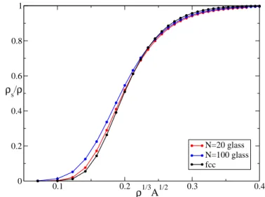
0.1 0.2 0.3 0.4 ρ1/3 A1/2 0 0.2 0.4 0.6 0.8 1 ρs/ρ N=20 glass N=100 glass fcc
FIG. 1: Leggett upper bound for ρs/ρ, for a Gaussian profile
of width A1/2 around an amorphous jammed configuration
and in a FCC lattice, as a function of the adimensional pa-rameter ℓ = ρ1/3A1/2(the Lindemann ratio).
hard spheres. Although this certainly is not a realis-tic model of density profiles for He4, it allows us to
ad-dress the role of disorder on ρs. Furthermore, a mapping
from quantum systems at zero temperature and classi-cal Brownian systems allows one to find quantum many particle models whose ground state wave-function can be mapped exactly on (the square of) the probability distri-bution of classical hard spheres systems [13]. Thus, the results of this section apply directly to those models.
Classical hard spheres are known to be characterized by a high density crystal FCC phase. However, if com-pressed fast enough, or due to a small polydispersity, the hard spheres freeze in an amorphous glassy state. A typ-ical density profile of a very quickly compressed glassy state can be obtained by the Lubachevski-Stillinger com-pression algorithm [21] (we used the implementation of [22]), which is know to be very efficient in producing amorphous jammed configurations. The output of the algorithm are the positions R = {R1,· · · , RN} of the
particles in a random close packed state (at infinite pres-sure). The algorithm is deterministic, but different final configurations are obtained by starting the compression from random initial configurations of points. The com-pression runs were performed at very fast rates (we fixed the parameter γ = 0.1, see [22, 23] for details) in order to avoid crystallization.
Furthermore, we will assume that the density profile of a typical glassy configuration at finite pressure is the sum of Gaussians centered around the amorphous sites, which are the output of the previous algorithm. For classical systems, this assumption has been tested numerically for FCC crystals [24], and has been often used in density functional computations of both ordered [25] and amor-phous structures [23, 26], giving accurate results. For
quantum systems, the Gaussian model has been shown to be accurate enough, at least for the purpose of com-puting the Leggett’s upper bound [27–29].
For a given configurationR, the density profile we use is defined as ρ(~r|R) =X i γA(|~r− ~Ri|) = Z V d~s γA(|~r−~s|) X i δ(~s− ~Ri) , (8) where γA(~x) = exp(−|~x|2/(2A))/(2πA)3/2 is a
normal-ized Gaussian of width A, and|~r − ~Ri| is the distance on
the periodic box, i.e. it is the distance between ~r and its closest image of ~Ri. The corresponding Fourier transform
reads (neglecting terms of order exp(−L2/A)):
ρ~q(R) = e−Aq 2 /21 V X i ei~q· ~Ri . (9)
In solving Eqs. (6) and (7) we considered amorphous configurations of N = 20 and N = 100 particles. All the calculations were done with the cut-off set at qmax=
20π/L. We checked that the result does not depend on the specific amorphous configuration used by considering different amorphous configurations Rα, α = 1,
· · · , N ; this is expected since the superfluid density is a macro-scopic quantity. The reported results are therefore av-eraged over 10 independent configurations. More details on the numerics can be found in Appendix A.
The results are plotted in Figure 1. One can notice that, apart from the smallest values of the dimension-less parameter, the two curves corresponding to 20 and 100 particle configurations perfectly agree. The discrep-ancy in the region of small ℓ = ρ1/3A1/2 is due to the
approximation brought by the introduction of a cut-off, and vanishes in the limit qmax≫ 1/√A.
In order to understand to what extent the disorder in-fluences the value of the superfluid density, we compare the superfluid fraction found in the amorphous system to the values obtained through the same calculations in the case of a crystal [17, 27–29]. Figure 1 reports the re-sults for the average superfluid fraction of the amorphous solid just described and those corresponding to the FCC lattice (which is the thermodynamically stable one for hard spheres) for the ~Ri, according to the same
Gaus-sian model (in the latter case our results are consistent with previous ones [17, 27–29]). The difference between the two is very small, suggesting two conclusions.
1. Disorder does not influence much the superfluid behavior of the system for comparable values of ρ1/3A1/2, at least at the level of this variational
calculation.
2. The dependence of ρs on the density profile is
mainly through the Lindemann ratio ℓ = ρ1/3A1/2. This conjecture allows us to obtain an estimate of the Leggett upper bound for ρs in more realistic
cases as we will do in the next section.
To conclude this section, we observe that the above re-sults allow to obtain a quantitative upper bound for the superfluid fraction of a system whose wavefunction is ex-actly the Jastrow wavefunction corresponding to classical hard spheres. The quantum glassy phase of this system has been discussed in [13]. In both the crystal and glassy phases, the values of A1/2 for classical hard spheres do
not exceed 0.1 (in units of the sphere diameter) [23–25], and the same is true for ℓ, since the density is very close to 1 (in the same units) in both solid phases. Using the results of Fig. 1, we obtain an upper bound ρs/ρ <∼ 0.1%,
which is consistent with the extremely small values of the condensate fraction found in [13].
B. Superfluid fraction of amorphous solid Helium 4
In this section, we attempt an application of our results to the more interesting case of disordered solid He4, based
on the observation above, that an estimate of the Linde-mann ratio ℓ = ρ1/3A1/2, together with the results of
Fig. 1, should provide a reasonable estimate of Leggett’s bound.
At the end of Ref.[29] it is stated that, by fitting the Path Integral Monte Carlo density profile of HCP solid He4, one obtains a value √A = 0.1274 d at ρ =
0.0353 ˚A−3 and √A = 0.1486 d at ρ = 0.029 ˚A−3.
Here d is the nearest-neighbor distance for the HCP lattice. The number density of the HCP lattice satis-fies the relation ρd3 = √2, hence d = 21/6/ρ1/3 and
ℓ =√Aρ1/3= 21/6√A/d. In the same reference it is also
stated that the upper bound computed by using the fitted Gaussian density profile coincides with the one obtained by using the true PIMC density profile, and corresponds respectively to ρs/ρ = 0.06 and 0.22. These values are
reported in table I.
We now make the following assumptions:
1. At least for the purpose of computing Leggett’s up-per bound, the true density profile can be fitted to a Gaussian profile. This is true for the crystal [29] and we assume that it remains true for an amor-phous solid.
2. The parameter ℓ for the amorphous solid is smaller than that of the crystal at the same density. This can be understood by observing that crystalline configurations are better packed than amorphous configurations, therefore leaving more room (“free volume”) for fluctuations. It is true for Jastrow wavefunctions [13] (i.e. classical system) and we do not find any reason why quantum fluctuations should dramatically affect this property.
Based on these assumptions, the true Leggett’s bound for the amorphous system should be smaller than the same bound for the crystal at the same density. This can be estimated using the values of ℓ reported in [29] and reading the corresponding superfluid fraction from Fig. 1
HCP, Leggett’s bound (Ref.[29]) Glass, Leggett’s bound (this work) Glass, QMC (Ref. [6])
ρ (˚A−3) ℓ ρ
s/ρ ρs/ρ ρs/ρ
0.029 0.167 0.22 0.282 0.6
0.0353 0.143 0.06 0.127 0.07
TABLE I: Leggett’s bound for He4
in the HCP crystal state [29] and glassy state. Quantum Monte Carlo results for the glass are also reported [6].
or using the results obtained in [29] for the HCP crystal. These values are reported in table I and are similar.
We compare the upper bound obtained in this way with the values of ρs obtained numerically by Boninsegni et
al. via PIMC [6]. Interestingly, we find that the bound is very close to the PIMC numerical result, and in particu-lar at the smallest density the bound is violated by the PIMC result. This can be due either to the very rough approximations involved in our computation, or to the fact that the glass is not a really long-lived metastable state at this very low density. The latter possibility, i.e. that the system is rapidly evolving out of equilibrium, would invalidate the derivation of Leggett’s bound but it would also raise problematic questions regarding the measurement of ρs using the Ceperley formula, which is
strictly valid if thermodynamic equilibrium is achieved and in the limit of small frequency.
IV. DOES A STABLE GLASS STATE EXISTS
FOR HELIUM 4?
In order to study the stability of the glass phase in He-lium 4, we performed Path Integral Monte Carlo simula-tions, that we discuss in this section. Before discussing the more complex quantum simulation, we present some classical simulations in order to deal with a well con-trolled situation, where the presence of a glass transition has been firmly established.
1. What should we expect from a glass-forming system? A classical simulation
We performed standard Molecular Dynamics (MD) simulations of the Kob-Andersen binary mixture [14], which is known to be a good glass former and does not show any sign of crystallization even after very long MD runs at low temperature. The latter is a mixture of two types of particles (A and B), interacting through different Lennard-Jones potentials, with the parameters specified in [14]. In the rest of this section we use reduced Lennard-Jones units, namely we use σAA and εAA as units of
length and energy, and m as unit of mass. Consequently, p
mσ2
AA/εAA is the unit of time (the latter convention
is slightly different from the one of [14]). Note that to compare with Helium one should keep in mind that for that system σ∼ 2.56 ˚A and ε∼ 10.2 K.
We quenched a dense (ρ = 1.2) system of N = 216 particles from very high temperature (T = 2) to very low temperature (T = 0.05) deep in the glass phase (the glass transition temperature being around T = 0.435 at this density [14]). We run the simulation for a to-tal time τ = 15000 and we printed configurations every ∆t = 5 which is of the order of the decorrelation time in the glass (estimated from the decay of the self scattering functions). From each configuration we deduced
ρ~q(t) = 1 V X j ei~q·~rj(t) , (10)
where ~rj(t) is the position of particle j at time t, and the
corresponding instantaneous value of the static structure factor S~q(t) = V|ρ~q(t)|2/ρ.
In Fig. 2 we plotted ρ~q(t) and the structure factor S~q(t)
as a function of MD time after the quench. The vectors ~
q = 2π/L(nx, ny, nz) and the corresponding integers are
given in the caption. We see that after a short tran-sient, the density profiles fluctuate around a non-zero value which is quite stable, except for some rare “crack” events where the density changes abruptly. These are probably due to groups of particles that switch back and forth between two different locally stable configurations. This system is indeed extremely dense and at very low T , therefore its dynamics is basically that of harmonic vibrations around local minima of the potential (except for the rare cracks). The largest instantaneous value of S~q(t) corresponds to the (2, 1,−6) curve in Fig. 2 for all
t > 1000; therefore, all values are smaller than 20 at all times, showing that there are no Bragg peaks. This is what we expect to see in a glass. In this case, we can easily deduce the average values of ρ~q for a given glassy
configurations by taking the average of ρ~q(t) over a time
interval where there are no crack events. From these, we could compute the Leggett bound as previously dis-cussed.
2. Absence of a stable glass phase from a Path Integral Monte Carlo simulation
Motivated by results of [6] we tried to compute the superfluid fraction based directly on Path Integral Monte Carlo data. Unfortunately, PIMC does not give access to the real time dynamics of the system, but following [6] we studied the Monte Carlo dynamics, in the hope that this is a reasonable proxy for the real time dynamics.
0 5000 t 10000 15000 0 5 10 15 20 25 S q(t) (1,7,0) (0,0,8) (2,1,-6) 0 5000 t 10000 15000 -0.2 -0.1 0 0.1 0.2 (0,0,8) Re ρq(t) Im ρ q(t) 0 5 q 10 15 0 5 10 15 20 S(q)
FIG. 2: Evolution of the density profile after a quench from high to low temperature for a classical glass forming sys-tem, using Molecular Dynamics. (Top) Instantaneous value of S~q(t) for three representative values of ~q (the corresponding
(nx, ny, nz) are indicated in the caption). (Middle)
Instanta-neous values of ρ~q(t) for a representative value of ~q. (Bottom)
The time average of S~q(t) over the whole simulation, as a
func-tion of q (in reduced LJ units). Scatter points are values for a given ~q, the full black line is the angular average over all vectors with the same modulus.
0 50000 t 100000 0 10 20 30 40 50 60 S q(t) (0,0,6) (5,0,4) (5,4,2) 0 50000 t 100000 -0.03 -0.02 -0.01 0 0.01 0.02 0.03 (0,0,6) Re ρq(t) Im ρq(t) 0 1 2 q 3 4 0 10 20 30 40 50 S(q)
FIG. 3: Evolution of the density profile after a quench from high to low temperature for a quantum Helium 4 system, using Path Integral Monte Carlo. Time here represents the number of Monte Carlo sweeps. The panels are the same as in Fig. 2, except that the average of S~q(t) in the lower panel
has been taken for t > 75000, and the angular average is not reported because of the strong anisotropy of the result. All quantities are plotted using ˚A as units of length.
The representation of quantum systems in PIMC in-volves certain important extensions beyond the classical representation of point particles. To begin with, particles are represented by paths (or polymers) in space. These paths manifest the zero point motion inherent in the quantum mechanical system. For distinguishable parti-cles, this is the only difference. For particles with statis-tics (bosons), these paths then can permute onto each other forming larger paths or cycles.
We initially focus on studying a quenched quantum system of Helium particles but require that they act like distinguishable particles. There are a number of poten-tial advantages of this approach. To begin with, one may hope that distinguishable particles are more likely to retain the relationship between real dynamics and the Monte Carlo dynamics. Secondly, the simulation of distinguishable particles is faster and more easily paral-lelized over many processors allowing for longer simula-tions.
We used the Aziz potential as a model for Helium [30], and in this section we always use Angstroms as units of length and Kelvins as units of temperature. The pair product action is used as the approximation for the high temperature density matrix and an imaginary time step of δτ = 0.025 K is used. We equilibrated a system of N = 216 particles in the liquid phase at a density of 0.029 ˚A−1 and a temperature of T = 2 K. The system
is then instantaneously quenched to T = 0.166 K. This is accomplished by taking a snapshot of the paths from T = 2 K and then, for each time slice of the old path, placing 12 time slices for the new lower temperature path; this is similar to what was done by Boninsegni et al. [6]. We then run the PIMC from this quenched configura-tion. These paths are obviously highly artificial because the distances between many adjacent time slices are zero. Over a very short period at the beginning of the quenched run, though, this artificial aspect of the path quickly re-laxes leaving the paths in a configuration that mirrors the higher temperature formation.
In the following we refer to t as the PIMC “time” (num-ber of PIMC sweeps1), while τ is the imaginary time. At
each “time” t, the PIMC code returns a configuration ~rτ
j(t), the latter being the imaginary time trajectory of
particle j as function of the imaginary time τ . We can define the instantaneous density as
ρ~q(t) = 1 βV X j Z β 0 dτ ei~q·~rτj(t) , (11)
and the instantaneous structure factor S~q(t) = 1 βN X j,k Z β 0 dτ ei~q·[~rτj(t)−~r τ k(t)] . (12) 1
We define a sweep as attempting a displace move on (an ex-pected) 10% of the particles and attempting bisection moves on (not necessarily unique) 0.4N/(T δτ ) time slices.
Note that in the quantum case, at variance with the clas-sical case, these two quantities are not directly related. At each PIMC sweep we recorded the values of the above quantities, which we then averaged over 50 PIMC sweeps in order to eliminate part of the fluctuations.
The results for a representative run of the above proce-dure are reported in Fig. 3. Unfortunately, the dynamics of this system looks quite different from the formation of a glass from a quenched liquid. First of all, the structure factor becomes quite large for some values of ~q, therefore suggesting the presence of large crystallites in the sam-ple. Indeed, the largest value of the structure factor cor-responds to the (5, 0, 4) curve in Fig. 3 at large times and to the (5, 4, 2) curve in Fig. 3 at short times. We see that while at short times the values of S~q(t) are smaller than
10, at larger times they grow up to 50, which clearly indi-cates the presence of large crystallites in the sample (note in addition that these values have been averaged over 50 PIMC sweeps and also over imaginary time). Moreover, the ρ~q(t) (reported for a representative value of ~q in the
middle panel of Fig. 3) are not fluctuating around some stable value; they display a sluggish evolution that does not allow us to identify a region of times where the system is close to some metastable density profile that does not evolve in time. What we can learn from this is that the quenching from a free) liquid to a (exchange-free) low temperature liquid froze to a (possibly very broken) crystal relatively quickly without showing any intermediate signs of glassiness. Note however that this behavior was not observed in all runs: some runs did not display signs of crystallization for times up to∼ 200000 PIMC sweeps. Still the dynamics was sluggish enough to prevent the identification of a stable glass phase. We also tried turning off some moves (the displace moves) in order to slow down the relaxation to the crystal, but the system still seems to freeze just as quickly.
In conclusions, we were not able to find a long-lived metastable glassy state in our quantum simulations. This is probably due to the fact that monodisperse systems al-ways crystallize quite fast. This is well known in the clas-sical case and seems to also hold true when quantum zero point motion is introduced (at least in this specific ex-ample). This leaves the discrepancy between our findings and those of [6] to be explained. One possibility is that exchange, that we neglected, may be critically important for exhibiting the glassy behavior of Helium 4: it could be that the path integral at the low temperatures we are focusing on is dominated by exchange paths, whereas the paths that make the glass unstable are mainly without exchange; indeed we find them with our PIMC. In this case, the instability of the glass would be a much rarer process once one takes into account exchange paths. In particular, since crystals have a very low or zero super-fluid fraction, we know that their corresponding path in-tegral is dominated by paths without exchange. In conse-quence, eliminating the exchange could also make crystal nucleation easier since it makes it a less rare process.
sensitive to the specific details of the simulation (type of Monte Carlo moves, length of the paths, etc.). We leave a more detailed investigation of this point for future study.
V. TOWARDS A METHOD FOR
EXPERIMENTALLY ASSESSING THE LEGGETT BOUND
As we discussed previously, the problem in applying our analysis to realistic system is that the amorphous density profile of He4 cannot be easily measured
experi-mentally. Below, we endeavor to connect the bound on ρsto the so-called non-ergodic factor egq, which in
princi-ple could be measured in experiments, e.g. by neutrons or X-ray scattering. It is defined as
ρ2 Negq = 1 N X α ρα~qρα−~q= ρ~qρ−~q , (13)
where the overbar denotes the statistical average over the amorphous states sampled statistically by the sys-tem. These are indexed by α = 1,· · · , N , and under the Gaussian approximation each profile ρα
~
q is obtained from
Eq. (9) by plugging the reference positions correspond-ing to each different amorphous configuration Rα. The
statistical average is performed with the weights α that correspond to the frequency with which they appear in an experiment, or equivalently their Boltzmann weight.
First, let us focus on ρs, which is the average of the
superfluid density ρα
s corresponding to each amorphous
state. Since the superfluid density is a macroscopic quan-tity we expect (and we have checked numerically, see Ap-pendix A) a self-averaging behavior, i.e. the fluctuations of ρα
s are negligible. However, as usual for disordered
systems, the computations are easier for ρs. Multiplying
Eq. (6) by ρα
−~q and averaging over α we obtain
(~q· ~v0) ρ2 Ngeq= X ~ p6=~0 (~q· ~p)F (~q, ~p) , (14)
where we define, for ~p, ~q 6= 0 (that are the only cases involved in the equation above)
F (~q, ~p) = 1 N
X
α
ρα~q−~piδϕα~pρα−~q = ρ~q−~piδϕ~pρ−~q . (15)
Clearly iϕ~q is strongly correlated to ρ~q, being the solution
of (6). In order to simplify the problem we assume that these variable are Gaussian distributed. Using Wick’s theorem, one has
F (~q, ~p) = ρ~q−~p iδϕp~ ρ−~q+ ρ~q−~p iδϕ~pρ−~q
+ ρ~q−~piδϕ~p ρ−~q+ ρ~q−~pρ−~q iδϕ~p .
(16) Note that, due to translation invariance of the averages over α, one has ρ~q = ρδ~q,~0 and ρ~qρ−~p= ρ
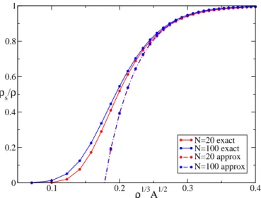
2 Negqδ~q,~p. Hence, 0.1 0.2 0.3 0.4 ρ1/3 A1/2 0 0.2 0.4 0.6 0.8 1 ρs/ρ N=20 exact N=100 exact N=20 approx N=100 approx
FIG. 4: Result for ρs/ρ as a function of ℓ = ρ 1/3
A1/2
, where ~
Ri are the center of the spheres in an amorphous jammed
configuration of N spheres with periodic boundary conditions. We report the exact computation according to Eq. (6) and the approximate result Eq. (20).
for ~p, ~q6= 0, we get
F (~q, ~p) = ρ~q−~p iδϕ~pρ−~q = ρδ~q,~piδϕ~qρ−~q ≡ ρδ~q,~pF (~q) .
(17) Substituting the last expression in (14), we obtain
F (~q) = ρ(~q· ~v0)egq
N q2 . (18)
Averaging (7) over α, we get ρs ρ = 1− 1 ρv2 0 X ~ q6=~0 (~v0· ~q)F (~q) = 1 − 1 N X ~ q6=~0 (~v0· ~q)2 v2 0q2 eg q . (19) In the thermodynamic limit, the sum can be replaced by an integral, and performing the angular integration we obtain: ρs ρ = 1− 2 3 Z ∞ 0 dq q2 (2π)2ρegq . (20)
The same result can be obtained by means of a large A expansion of the system of equations, which however is poorly convergent and cannot be used in a systematic way, see Appendix B.
As before we need to introduce a cut-off in the sum on ~
q in (9) and calculate numerically the non-ergodic factor egq by averaging the density over the same configurations
Rαconsidered above. We set the cutoff according to the
spherical constraint|~q| ≤ qmax. We increased qmaxuntil
qmax= 20π/L, when the convergence in egq was reached.
For the purpose of computing the non-ergodic factor and then the approximate bound, as given in Eq. (19), we averaged over 100 different configurations. In this case,
in fact, one does not face the computational problem of inverting the linear system (6) and thus a larger statistics can easily be taken. The results of the computations are shown in Figure 4. We plotted the superfluid fraction obtained through the exact procedure (7) and the ap-proximated one (20), both for the configurations with 20 and 100 particles. The agreement between the approx-imated curve and the exact one is good for large value of ℓ while they start to differ when the localization pa-rameter decreases, for values of the bound around 0.7. Unfortunately for the interesting values of ℓ the approxi-mated calculation gives wrong results. However, we find it useful, since it allows to estimate the typical scale of ℓ at which the bound starts decreasing fast from 1 to 0 and we hope that it will be possible to improve it in the future, in order to be able to apply it to realistic cases.
VI. CONCLUSIONS
The aim of this paper was to study Leggett’s upper bound for amorphous quantum solids. We showed that for quantum systems described by a hard sphere Jastrow wavefunction, the superfluid fraction must be smaller that 0.1%, which is consistent with a previous investi-gation that found extremely small condensate fractions for this system [13]. Moreover, the hard sphere result suggests that crystal and glass phase characterized by the same Lindemann ratio should have similar Leggett’s upper bounds for the superfluid fraction.
On this basis, we attempted to apply our results to glassy He4[6]. We found that the upper bound for ρ
s is
in general very close to the numerical results of Ref. [6], and at density ρ = 0.029 ˚A−3 it is below. One
possi-ble origin of this discrepancy could be that at such low density the life time of the metastable glassy state is too short, and the system is intrinsically out of equilib-rium; in that situation Leggett’s bound is inapplicable, since it assumes that the reference wave-function corre-sponds to a truly metastable state. Indeed we generically found from Path Integral Monte Carlo calculations that (at least if exchange is neglected) the system crystallizes very fast after the quench, which is consistent with a very short lifetime of the metastable glass.
Overall, our findings suggest two possible scenarios (not necessarly antithetic). (1) An amorphous stable glass has a superfluid fraction, not only a Leggett’s upper bound, very similar to a defect-free crystal with the same Lindemann ratio. Since we know from experiments and simulations that this superfluid fraction is very small, or possibly zero, we are bound to conclude that the glassy supersolid phase found in experiments do not cor-respond to a truly stable glass: the system is instead rapidly evolving out of equilibrium and, somehow, this enhances superfluidity. (2) Exchange promotes glassiness and whereas a stable glass phase cannot exist, because it has a very short life-time, a superglass can. This could be partially tested by comparing the stability of the glass
phase in imaginary time simulations with and without exchange.
It is worth to note that we neglected the role of small concentration of He3impurities (of the order of few ppm)
that has received a lot of attention in experiments [3]. The reason is that we focused on a bulk glass phase of He4, whose density profile should be largely independent
of such a small concentration of He3impurities. It could
be, however, that He3 impurities affect the dynamical
stability of the glass phase. Based on the experience on classical systems, it is likely that in presence of a large concentration of impurities crystallization will be avoided [14] and a long-lived quantum glass phase [15, 31] will be stable. In this case, it should be very easy to mea-sure the density profile and compute the Leggett bound using the procedure detailed above. However, it has been estimated that a concentration of at least 0.1% of im-purities is needed to stabilize the glass [32]. Therefore, the typical concentration of He3 (
∼ ppm) should not be enough to produce a sensible effect, unless some unex-pected phenomenon related to the quantum mechanical nature of the systems (e.g. exchange, as already dis-cussed) becomes relevant.
Acknowledgments
We wish to thank S. Baroni, M. Boninsegni, G. Car-leo, S. Moroni and L. Reatto for very useful discussions. FZ wishes to thank the Princeton Center for Theoreti-cal Science for hospitality during part of this work. This research was supported in part by the National Science Foundation under Grant No. NSF PHY05-51164. Part of the numerical calculations have been performed on the cluster “Titane” of CEA-Saclay under the grant GENCI 6418 (2010).
Appendix A: Details on the numerical procedure
We define the Fourier transforms in the cubic box of side L and volume V = L3 as follows:
ρ~q = 1 V Z V d~rρ(~r)ei~q·~r, ρ(~r) =X ~ q ρ~qe−i~q·~r, (A1) where ~q = 2π
L(nx, ny, nz), and each of the integers ni∈ Z,
and similarly δϕ~q = 1 V Z V d~rδϕ(~r)ei~q·~r . (A2) Note that δϕ~0is an irrelevant constant phase in the vari-ational wavefunction so we set it to zero. Finally,
~v~q =
(
~v0 ~q = ~0 ,
−i~qϕ~q ~q6= ~0 .
(A3) which leads immediately to Eq. (6).
We performed the calculations for different values of the Lindemann parameter ℓ = ρ1/3A1/2, increasing the
number of vectors ~q according to the spherical constraint |~q| ≤ qmax, until a reasonable convergence in the value
of the bound (7) was achieved, at least for large val-ues of A. From Eq. (9) one sees that for large |~q| the corresponding component ρ~q is suppressed through the
factor e−Aq2/2. Thus, one needs to truncate the sum over ~q at qmax ∼ 1/√A, as higher terms will not
con-tribute. Unfortunately, for small A, this cut-off is too heavy in terms of computational time and we should use a lower one. Still, considering small configurations and sufficiently large values of A, which nevertheless span the physical region of interest, we could reach a good conver-gence or keep the error under control. Note additionally that by increasing the number of vectors ~q in (9), the value found for the superfluid fraction monotonically de-creases, as expected because of the variational property already discussed. This permits to preserve the nature of upper bound for Eq. (7), despite the cut-off approxima-tion. Overall, we found that the better compromise was to set qmax= 20π/L.
In order to check the independence of the bound on the flow direction, we also compared the results obtained with the velocity v0along the (1, 0, 0) direction to those
along (1, 1, 1) and we observed a negligible difference which is expected to vanish in the thermodynamic limit, because amorphous solids are statistically homogeneous on large scales.
We have also checked that the bound for the superfluid density almost does not fluctuate by considering different amorphous configurationsRα, α = 1,
· · · , N , as it is ex-pected since the superfluid density is a macroscopic quan-tity. We computed the corresponding superfluid fraction ρα
s and the average ρs=
P
αραs/N for 10 different
config-urations. The variance of ρs is very small. In this paper
we presented results averaged over 10 realizations ofRα,
a larger statistics do not lead to appreciable differences. Finally, as a check of our codes, we repeated all the calculations on configurations of 20 particles occupying uncorrelated uniformly random positions in the box, i.e. where ~Ri are uniform and independent random
vari-ables in [0, L]3. In this case it is easy to show that
e
gq = exp(−Aq2). Hence Eq. (20) becomes
ρs ρ = 1− 2 3(2π)2ρ Z ∞ 0 dq q2e−Aq2 = 1−24π3/21ρA3/2 . (A4)
In this case the values of the bound were more sensitive to the particular realization, so we took averages over 30 configurations. For every value of the localization pa-rameter, the superfluid fractions that we found were on average smaller, as reported in Figure 5.
0 0.2 0.4 ρ1/3 A1/2 0 0.2 0.4 0.6 0.8 1 ρs/ρ N=20 exact N=20 approx Analytic approx
FIG. 5: Result for ρs/ρ as a function of the localization
pa-rameter ρ1/3
A1/2
, where ~Ri are N random points in [0, L] 3
with periodic boundary conditions.
Appendix B: Large A expansion
For large A, we expect that the density becomes uni-form. Hence, ρ~0→ ρ, and ρ~q → 0 for ~q 6= ~0. We can use
this to expand iδϕ~q systematically in powers of ρ~q. We
rewrite Eq. (6) as ~ q· ~v0ρ~q= q2ρiδϕ~q+ X ~ p6=~0,~q (~q· ~p)ρ~q−~piδϕ~p . (B1) We write δϕ~q = δϕ(1)~q + δϕ (2) ~
q +· · · where the different
terms are of order (ρ~q)k. At first order
iδϕ(1)~q = ~q· ~v0 q2ρ ρ~q , (B2) at second order iδϕ(2)~q =− 1 q2ρ X ~ p6=~0,~q (~q· ~p)ρ~q−~piδϕ(1)~p =− X ~ p6=~0,~q (~q· ~p)(~p · ~v0) p2q2ρ2 ρ~q−~pρ~p , (B3) at third order iϕ(3)~q =− 1 ~ q2ρ X ~ p6=~0,~q (~q· ~p)ρ~q−~piϕ(2)~p = X ~ p6=~0,~q X ~ p′6=~0,~p (~q· ~p)(~p · ~p′)(~p′ · ~v0) q2p2p′2ρ3 ρ~q−~pρ~p−~p′ρp~′ (B4)
from which we can guess the order k: iϕ(k)~q = (−1)k−1 X ~ p16=~0,~q; ~p26=~0,~p1; ··· ~pk−16=~0,~pk−2 (~q· ~p1)(~p1· ~p2)· · · (~pk−1· ~v0) q2p2 1· · · p2k−1ρk ρ~q−~p1ρp~1−~p2· · · ρp~k−2−~pk−1ρ~pk−1 (B5)
and so on. Plugging this in Eq. (7) we get ρs ρ =1− X ~ q6=~0 (~v0· ~q)2 ρ2v2 0q2 ρ~qρ−~q+ X ~ q6=~0 X ~ p6=~0,~q (~v0· ~q)(~q · ~p)(~p · ~v0) q2p2v2 0ρ3 ρ~q−~pρp~ρ−~q −X ~ q6=~0 X ~ p6=~0,~q X ~ p′6=~0,~p (~v0· ~q)(~q · ~p)(~p · ~p′)(~p′· ~v0) q2p2p′2v2 0ρ4 ρ~q−~pρ~p−~p′ρ~p′ρ−~q+· · · . (B6)
While this expansion seems a simple strategy of solution of Eq. (6), it is very poorly convergent and in practice it is not very helpful.
[1] E. Kim and M. H. W. Chan, Nature (London) 427, 225 (2004); E. Kim and M. H. W. Chan, Science 305, 1941 (2004).
[2] A. C. Clark, J. T. West, and M. H. W. Chan, Phys. Rev. Lett. 99, 135302 (2007).
[3] For reviews, see: D. Ceperley, Nature Physics 2, 659 (2006); N. V. Prokof’ev, Advances in Physics 56, 381 (2007); P. Phillips, A. Balatsky, Science 316, 1435 (2007); S. Balibar and F. Caupin, J. Phys.: Condens. Matter 20, 173201 (2008).
[4] D. M. Ceperley and B. Bernu, Phys. Rev. Lett. 93, 155303 (2004)
[5] N. Prokof’ev and B. Svistunov, Phys. Rev. Lett. 94, 155302 (2005).
[6] M. Boninsegni, N. Prokof’ev, and B. Svistunov, Phys. Rev. Lett. 96, 105301 (2006).
[7] A. S. Rittner and J.D. Reppy, Phys. Rev. Lett. 97, 165301 (2006).
[8] A. S. Rittner, J. D. Reppy, Phys. Rev. Lett. 98, 175302 (2007).
[9] Z. Nussinov, A. V. Balatsky, M. J. Graf, and S. A. Trug-man, Phys. Rev. B 76, 014530 (2007); C.-D. Yoo and A. T. Dorsey, Phys. Rev. B 79, 100504(R) (2009). [10] B. Hunt, E. Pratt, V. Gadagkar, M. Yamashita,
A. V. Balatsky, and J. C. Davis, Science 324, 632 (2009). [11] M. Boninsegni, A. Kuklov, L. Pollet, N. Prokof’ev, B. Svistunov, M. Troyer, Phys. Rev. Lett. 97, 080401 (2006).
[12] M. Rossi, E. Vitali, D.E. Galli, L. Reatto, J. Low Temp. Phys. 153 (2008) 250.
[13] G. Biroli, C. Chamon and F. Zamponi, Phys.Rev.B 78, 224306 (2008).
[14] W. Kob and H. C. Andersen, Phys. Rev. E 51, 4626 (1995).
[15] T. E. Markland, J. A. Morrone, B. J. Berne, K. Miyazaki, E. Rabani, D. R. Reichman, Nature Physics, published
online (2010); arXiv:1011.0015.
[16] A. J. Leggett, Phys.Rev.Lett. 25, 1543 (1970). [17] W. M. Saslow, Phys.Rev.Lett. 36, 1151 (1976).
[18] W.M. Saslow, D.E. Galli, and L. Reatto, Journal of Low Temperature Physics 149, 53 (2007).
[19] D. Forster, Hydrodynamic fluctuations, broken
symme-try, and correlation functions, Westview Press (1995)
[20] Numerical recipes: the art of scientific computing, Cam-bridge University Press (2007).
[21] B. D. Lubachevsky and F. H. Stillinger, J. Stat. Phys. 60, 561 (1990).
[22] A. Donev, S. Torquato and F. H. Stillinger, Journal of Computational Physics 202, 737 (2005).
[23] G. Parisi and F. Zamponi, Rev. Mod. Phys. 82, 789 (2010).
[24] D. A. Young and B. J. Adler, J. Chem. Phys. 60, 1254 (1974).
[25] A. R. Denton, N. W. Ashcroft, W. A. Curtin, Phys. Rev. E 51, 65 (1995).
[26] J. P. Stoessel and P. G. Wolynes, J.Chem.Phys. 80, 4502 (1984).
[27] J. F. Fernandez and M. Puma, J. Low. Temp. Phys. 17, 131 (1974).
[28] W. M. Saslow and S. Jolad, Phys. Rev. B 73, 092505 (2006).
[29] D. E. Galli, L. Reatto and W. M. Saslow, Phys.Rev.B 76, 052503 (2007).
[30] D. M. Ceperley, Rev. Mod. Phys. 67, 279 (1995). [31] L. Foini, G. Semerjian, F. Zamponi, to be published on
Phys.Rev.B; arXiv:1011.6320
[32] Ya. E. Ryabov, Y. Hayashi, A. Gutina, and Y. Feldman, Phys. Rev. B 67, 132202 (2003); J. S. Yu, Y. Q. Zeng, T. Fujita, T. Hashizume, A. Inoue, T. Sakurai, and M. W. Chen, Appl. Phys. Lett. 96, 141901 (2010).
![TABLE I: Leggett’s bound for He 4 in the HCP crystal state [29] and glassy state. Quantum Monte Carlo results for the glass are also reported [6].](https://thumb-eu.123doks.com/thumbv2/123doknet/12721655.356688/6.918.154.779.75.157/table-leggett-crystal-glassy-quantum-monte-results-reported.webp)

![FIG. 5: Result for ρ s /ρ as a function of the localization pa- pa-rameter ρ 1 / 3 A 1 / 2 , where R~ i are N random points in [0, L] 3 with periodic boundary conditions.](https://thumb-eu.123doks.com/thumbv2/123doknet/12721655.356688/11.918.479.845.174.460/result-function-localization-rameter-random-periodic-boundary-conditions.webp)
