Stride lengths, speed and energy costs in
walking of
Australopithecus afarensis:
using evolutionary robotics to predict
locomotion of early human ancestors
William I. Sellers
1,†, Gemma M. Cain
1, Weijie Wang
2and Robin H. Crompton
31Department of Human Sciences, Loughborough University, Loughborough LE11 3TU, UK 2Section of Oncology and Surgery, Ninewells Medical School,
Institute of Motion Analysis and Research, University of Dundee, Dundee DD1 9SY, UK
3School of Biomedical Sciences, Sherrington Buildings, University of Liverpool,
Liverpool L69 3GE, UK
This paper uses techniques from evolutionary robotics to predict the most energy-efficient upright walking gait for the early human relative Australopithecus afarensis, based on the proportions of the 3.2 million year old AL 288-1 ‘Lucy’ skeleton, and matches predictions against the nearly contemporaneous (3.5–3.6 million year old) Laetoli fossil footprint trails. The technique creates gaits de novo and uses genetic algorithm optimization to search for the most efficient patterns of simulated muscular contraction at a variety of speeds. The model was first verified by predicting gaits for living human subjects, and comparing costs, stride lengths and speeds to experimentally determined values for the same subjects. Subsequent simulations for A. afarensis yield estimates of the range of walking speeds from 0.6 to 1.3 m sK1 at a cost of 7.0 J kgK1mK1 for the lowest speeds, falling to 5.8 J kgK1mK1 at 1.0 m sK1, and rising to 6.2 J kgK1mK1at the maximum speed achieved. Speeds previously estimated for the makers of the Laetoli footprint trails (0.56 or 0.64 m sK1for Trail 1, 0.72 or 0.75 m sK1for Trail 2/3) may have been underestimated, substantially so for Trail 2/3, with true values in excess of 0.7 and 1.0 m sK1, respectively. The predictions conflict with suggestions that A. afarensis used a ‘shuffling’ gait, indicating rather that the species was a fully competent biped.
Keywords: biomechanics; bipedalism; gait; evolution; palaeontology; simulation
1. INTRODUCTION
The adoption of bipedalism as the preferred mode of terrestrial locomotion is a fundamental step in diver-gence of the human lineage from that of other African apes. Human walking is characterized by extended postures of the hip and knee joints so that gait is relatively ‘stiff’. This ‘stiff’ gait brings about out-of-phase oscillations of the kinetic and potential energies of the centre of mass (CM) which permit energy to be exchanged between the two states conserving up to 70% of the energy of one stride for use in the next. There are, however, transitory knee-flexions at heel-strike, mid-stance and toe-off, which reduce both excessive vertical displacement of the body CM and peak vertical ground reaction forces. Bipedally walking chimpanzees by contrast use ‘compliant’ gaits where knee-flexions are sufficient and long-lasting enough to bring the oscil-lations of kinetic and potential energies of the CM into
phase, eliminating mechanical energy exchange, and thus increasing metabolic costs. When walking biped-ally the orang-utan does maintain extended hip and knee joints (Crompton et al. 2003) and up to 52% energy exchange occurs, but no ape appears to be able to combine extended hindlimb posture with the long strides and high stride frequencies that are required for fast bipedal walking. Human foot function also differs from that of other apes in that thrust is imparted to the ground by the fore-foot, maximizing leverage of triceps surae, the major muscle powering heel-off and toe-off. Other apes achieve peak plantar pressures and deliver thrust in the mid-foot, reducing leverage about the ankle joint. Thus the important locomotor innovation characterizing the human lineage is likely to be the development of a long, forceful and yet efficient stride rather than upright walking per se. When did this occur? There are unfortunately only a limited number of feet in the fossil record of early human ancestors: the most complete is the Homo habilis foot OH 8, dating to about 1.8 million years old. This is contemporaneous
doi:10.1098/rsif.2005.0060 Published online 18 July 2005
with a very modern looking, skeleton, WT 15 000, of Homo ergaster. WT 15 000 was clearly a human-like striding biped but, while otherwise nearly complete, lacks feet.
Recent analyses of the OH 8 foot suggested it is ‘ape-like’ on the medial side, lacking an arch and having a mobile midfoot and opposable big toe (Kidd 1995) but ‘human-like’ with a stabilized midfoot, on the lateral side. Older material exists for the early human ancestor Australopithecus afarensis, dating to about 2–3.2 million years old. The partial feet of skeletons AL 288-1 and AL 333 also appear to lack a medial arch, and the Australopithecus Sts 573 foot specimen again shows an apparent ‘mix’ of ‘human-like’ and ‘ape-like’ features (Harcourt-Smith & Aiello 2004).
Direct evidence of foot function in human ancestors at the time of Sts 573 and A. afarensis is provided by the Laetoli footprint trails (3.5–3.8 million years old) made in wet volcanic ashfall deposits (Hay 1987). While Trail A, with short, broad, and poorly defined prints, and stride length resembling that of a 2.5 year old human child, may not represent a human ancestor, but instead have been made by the extinct ursid (bear ancestor) Agriotherium africanus (Robbins 1987), Trail G1 represents at least four complete cycles of bipedal walking by a small individual of a human ancestor, most likely a child. Alongside it run two partly superimposed trails G2 and G3, with very similar morphology but wider spacing, which are likely to represent adults of the same species. White (1980)
regarded the Laetoli G prints as consistent with authorship by A. afarensis on the basis of the documented relationship of adult human skeletal stature to adult human footprint length. Jungers (1982) argued, however, that the short legs of A. afarensis, as represented by the famous ‘Lucy’ skeleton AL 288-1 implied short stride lengths like those in bipedal walking of the living non-human apes. Recently discovered but as yet undescribed postcranial material of Australopithecus from about four million years ago, and apparently of considerably greater stature, may yet prove to have been responsible for the Laetoli prints, but at present A. afarensis remains the best contemporaneous size-match for the Laetoli prints and the most likely maker. Stern & Sussman (1983)suggested that A. afarensis would have walked ‘bent-hip, bent-knee’ (BHBK), rather like a living chimpanzee, because of the number of skeletal features in the A. afarensis skeleton which are functionally associated with arboreality in living apes (e.g. curved phalanges, long trunk but short legs, etc.).Hunt (1994)
has even proposed that the most efficient behaviour for A. afarensis would have been ‘bipedal posture augmented with bipedal shuffling’ as a consequence of anatomical compromise between the needs of terrestrial bipedality and arboreal climbing. However, other authors (e.g. Latimer 1991) stress characteristics associated in humans with habitual bipedalism (such as a femur where the shaft is angulated to bring the knees under the centre of gravity of the body) and conclude that this species was an habitual, erect biped. This view is now becoming the general consensus (see e.g.Ward 2002).
Many of the disputes which surround the evolution of human bipedalism arise because there is no other living analogue for early bipeds but modern humans, while the body proportions of A. afarensis, for example, are so different from our own (short legs and long trunk versus our own long legs and short trunk) that the mechanics of motion must have been very different (e.g.
Alexander 2004). Rather than trying to interpret the behaviour of such species by a combination of analogies to humans in certain anatomical regions with analogies to other apes elsewhere, it seems sensible to adopt a reverse-engineering approach and determine what kind of locomotion a particular set of body proportions were best ‘designed’ to perform. Since the locomotor system is concerned primarily with the application of external force by the body, simulation techniques drawn from mechanical engineering are a potential means of predicting the significance of differences in proportions for the motion and force characteristics of bipedal locomotion.
There are two main techniques for investigating locomotor mechanics: inverse dynamics where forces are calculated based on observed movement and forward dynamics where movement is calculated based on applied forces (for review seevan den Bogert 1994). In an earlier study we showed using inverse dynamic modelling that the skeletal proportions of A. afarensis (AL 288-1) were compatible with stable and efficient upright bipedalism (Crompton et al. 1998) but that mechanical energy costs of locomotion were near-doubled in BHBK gait. (Carey & Crompton 2005
have since confirmed for humans that physiological costs are indeed much higher in BHBK gait).Kramer (1999)andKramer & Eck (2000)used similar inverse-dynamic techniques and also concluded that this species could have been an efficient upright biped. While inverse dynamics is computationally economical and has usefully been applied to assessing alternative hypotheses as to the gait of early human ancestors (Crompton et al. 1998; Kramer 1999; Kramer & Eck 2000; Wang et al. 2004) it requires that given sets of joint motions are applied to given sets of body proportions. This is not entirely satisfactory as while we often have fossil evidence of body proportions joint motion is of course not directly preserved in the fossil record. Moreover inverse dynamics can only be used for direct estimates of mechanical work. The relationship between mechanical work and metabolic energy cost is complex. For example muscles require energy to generate force even when no mechanical work is being performed or even when doing so-called ‘negative work’ (Winter 1990). However, recent advances in our ability to model muscle energetics (Minetti & Alexander 1997;
Umberger et al. 2003) together with the greater availability of facilities for computationally intensive modelling have together facilitated adoption of forwards dynamic modelling. This approach does not require imposition of given sets of joint kinematics but rather predicts them from body proportions and muscle activation patterns. Musculoskeletal model based forwards dynamics simulations can calculate metabolic energy costs directly, and have been shown to produce reliable results in human walking (Sellers et al. 2003).
Results have also been reported for A. afarensis (Sellers et al. 2004;Nagano et al. 2005). Since they use a finite-state controller to activate the muscles in the model and hence to drive bipedal locomotion, the approach adopted by the both groups need make no assumptions concerning the pattern of muscle activation.
Sellers and colleagues (2003, 2004) set the search pattern to maximize locomotor efficiency; Nagano et al. (2005), however, sought to match a predefined kinematic configuration at the start and end of a step whilst simultaneously minimizing the metabolic energy consumed per unit distance travelled during the step. There are merits to both approaches. In the former the model is free to select any kinematic pattern which can produce forward motion and therefore makes no assumptions about the correct kinematics for the fossil animal. In the latter there are some limited assump-tions about the required kinematics but these can considerably reduce the size of the search space and may improve gait cycle repeatability, allowing a much more complex model to be constructed. However, since the model constrains certain kinematic features such as speed and stride length it cannot easily be used to investigate the preferred speeds and stride lengths that suit the mechanics of the fossil (Nagano et al. 2005).
Our optimization method is drawn from evolution-ary robotics, a technique for the automatic creation of autonomous robots (Nolfi & Floreano 2000). Whilst primarily concentrating on navigation and learning issues, evolutionary robotics also covers the spon-taneous generation of locomotion in legged robots. It is therefore a tool with which we can investigate the locomotion of fossil animals. In this case values for segment proportions, joint mobilities, and muscle arrangements are either derived directly from the fossil evidence or represent anatomically likely values. A gait controller is used to activate the muscles to produce the required locomotion. Building the simulator is rela-tively straightforward computationally but finding an appropriate pattern to produce stable gait is difficult because the number of possible patterns is far too large for them all to be tested individually. However, such problems can be addressed effectively using genetic algorithms.
Evolutionary processes have led to highly optimized solutions to complex problems: thus, since the 1950s evolutionary theory has been used by computer scientists as a source of inspiration for optimization and machine learning algorithms. Evolutionary strat-egies (Rechenberg 1965) are the most developed of the early techniques. They encode the problem under consideration as a sequence of real numbers and then randomly mutate these numbers. Each time a mutation is created it is compared with the previous solution and if it performs better according to some metric criterion it replaces the original solution; otherwise it is discarded. By using a Gaussian mutation (adding a random value selected from a Gaussian probability distribution with a mean of zero) it is possible to generate any sequence, although the new sequences are more likely to be similar to the previous sequence than otherwise. This approach takes advantage of the fact that sequences close to the ‘best’ solution are likely to
be similar to that solution. Genetic Algorithms were invented by John Holland in the 1960s (Holland 1975). The genetic algorithm uses a population of solutions. Members of this population (called chromosomes) are allowed to contribute to the next generation by crossover, whereby two chromosomes exchange sub-sequences to create two new chromosomes. The selection of parent chromosomes is done randomly but is influenced by their fitness which is calculated in some way by a fitness function. The genetic algorithm sensu strictu uses a fixed length sequence of bits (zeros or ones) as its chromosome. However, the genetic algor-ithm has had such a large impact on the field of evolutionary computation that concepts such as popu-lations and crossover have been incorporated into other techniques and the term is now used to cover almost any population-based evolutionary search technique (for a more thorough introduction to genetic algorithms see Davis 1991). These evolutionary techniques have been widely used for difficult computational search problems and are ideal for finding sets of parameters in gait controllers that produce high quality gaits. An additional advantage is that because they work on populations of solutions they are ideal for parallel implementation, and thus allow extremely high per-formance (van Soest & Casius 2003).
This study therefore applies forwards dynamic analysis and genetic algorithm optimization to recon-struct the metabolic costs associated with different stride lengths and speeds for A. afarensis, on the assumption that this species walked upright, following
Nagano et al. (2005)and go on to apply our results to interpretation of the Laetoli footprint trails, assuming again that A. afarensis was the maker.
2. METHOD
It is extremely important that simulation studies are validated against experimental data wherever possible. Therefore, the first step in this study was to obtain such data experimentally for human subjects and to produce simulations based on those particular subjects’ morphology to allow direct comparison between exper-imental and simulated values. This will then allow us to evaluate the likely accuracy of any subsequent A. afarensis simulation.
To obtain the required experimental data five healthy young adult male human subjects were required to walk on a treadmill at speeds from 0.5 to 2.0 m sK1, in 0.25 m sK1 increments covering the subjects’ full range of walking speeds. The subjects were asked to walk at each speed for several minutes to allow the oxygen consumption rate to reach equili-brium. Then the subjects’ expired air was collected using a Douglas bag and analysed to estimate metabolic power using theWeir (1949)formula. Simultaneously, the subjects’ stride length was calculated by measuring the time taken for 30 strides. In addition the subjects’ metabolic rate was also measured standing (i.e. progressing at 0 m sK1) to allow the calculation of net locomotor costs (Heglund & Schepens 2003). The subjects were then weighed and the distances between neighbouring joint centres (first metatarsal head, ankle,
knee and hip and also the shoulder joint) were measured to allow calculation of the segment inertial properties using the formulae recommended by Winter (Winter 1990).
Five separate computer simulations were then constructed to match the morphology of the subjects. Due to the non-deterministic nature of the modelling process they were each run multiple times. The basic design was the same as we have used previously (Sellers et al. 2003, 2004) with three segment left and right hindlimbs (foot, leg and thigh) and a unified head, arms and truck (HAT) segment. The segment lengths were customized to match those of the human subjects, and assigned the calculated inertial properties (table 1).
Since this is a two-dimensional simulation the joints were all defined as hinge joints with appropriate ranges of motion (Delp et al. 1990). Muscles were grouped as primary flexors and extensors around the hip, knee and ankle joints; and muscle physiological cross section areas and fibre lengths of the groups were assigned by identifying the actions of the muscle and calculating a weighted average based on the physiological cross sectional area (PCSA) for each muscle contributing to the group based on data for individual muscles (Pierrynowski 1995). Attachment points were assigned based on the estimated centroid of the attachment area for a muscle group. For the knee extensor and flexors a wrapping operator was used to maintain the moment arm around the joint at an estimated 6 and 3 cm. The tendon lengths were calculated so that the muscle fibre length plus the tendon length was equal to the total path length in the anatomical position. The muscle model used was that of Umberger and colleagues (2003), based on FORTRAN code kindly supplied by
Umberger. This model also requires an estimate of serial and parallel elastic properties: these were calculated assuming a 6% strain in the tendon, and a 60% strain in the passive connective tissue component
of the muscle at its maximum isometric contraction, since these values appear to be typical of vertebrate skeletal muscle (Biewener 2003). The other values required for the model were set based on mean values for lower-limb muscles (Nagano & Gerritsen 2001;
Umberger et al. 2003). The values used are shown in
tables 2 and 3.
The A. afarensis model was produced from the human model by scaling the latter to the proportions of the AL 288-1 fossil skeleton (Johanson et al. 1982). A number of similar models have been produced pre-viously (Crompton et al. 1998;Kramer 1999;Kramer & Eck 2000;Sellers et al. 2004;Wang et al. 2004;Nagano et al. 2005) although all differ in the numerical values chosen for various parameters. Segment lengths (the distance between joint centres rather than the lengths of the bones themselves) were those adopted byKramer (1999) except for the HAT length (defined as the distance from the hip to the shoulder joint centre) which was estimated from the Lovejoy reconstruction (Weaver et al. 1985). There is considerable disagree-ment in literature concerning estimated total body weights: values vary from 12.3 to 38.9 kg (Aiello & Dean 1990). The simulations listed above all use values close to 30 kg; we chose 33 kg followingKramer (1999). In our previous work we reconstructed the inertial parameters of the segments based on both modern human and modern chimpanzee values. However, we found very little effect of mass distribution on results (Sellers et al. 2004) so in this paper we used human values reconstructed according to Winter’s method (Winter 1990). Muscle values were obtained directly by scaling from the human values since we have no way of estimating these soft tissue parameters. The muscle length was scaled based on the segment-length scaling from the human to the AL 288-1 models, while muscle PCSA was scaled so that relative muscle volume was maintained (i.e. area scaleZmass scale/length scale).
Table 1. The values for the inertial properties of the segments used in the computer simulation models.
(HAT length is from hip joint to shoulder joint, thigh from hip joint to knee joint, leg from knee joint to ankle joint, foot from ankle joint to first metatarsal head. CM position is the distance along the length of the segment (distally for the leg segments and cranially for the HAT segment). Moments of inertia are about the local origin of each segment which is the proximal joint except for the HAT which is about the hip joint.)
subject 1 subject 2 subject 3 subject 4 subject 5 AL 288-1
HAT mass (kg) 50.7144 56.7147 60.2403 38.9850 53.8671 22.3740 length (m) 0.5490 0.5020 0.5190 0.4850 0.4920 0.3516 MOI (kg m2) 9.7338 9.1014 10.3330 5.8396 8.3035 1.7610 CM (m) 0.3437 0.3143 0.3249 0.3036 0.3080 0.2201 thigh mass (kg) 7.4800 8.3650 8.8850 5.7500 7.9450 3.3000 length (m) 0.4550 0.3940 0.4470 0.4100 0.4760 0.2520 MOI (kg m2) 0.4516 0.3787 0.5177 0.2819 0.5249 0.0611 CM (m) 0.1970 0.1706 0.1936 0.1775 0.2061 0.1091 leg mass (kg) 3.4782 3.8897 4.1315 2.6738 3.6944 1.5350 length (m) 0.4520 0.3980 0.4370 0.3150 0.4790 0.2650 MOI (kg m2) 0.1981 0.1718 0.2200 0.0740 0.2363 0.0300 CM (m) 0.1957 0.1723 0.1892 0.1364 0.2074 0.1150 foot mass (kg) 1.0846 1.2129 1.2883 0.8338 1.1520 0.4790 length (m) 0.1690 0.1340 0.1480 0.1290 0.1530 0.0800 MOI (kg m2) 0.0147 0.0104 0.0134 0.0066 0.0128 0.0015 CM (m) 0.0845 0.0670 0.0740 0.0645 0.0765 0.0400
Knee moment arms were reduced to 4 and 2 cm. The values used are shown intables 1 and 2.
The biomechanical simulation is performed using custom-written software written in CCC using the open-source Dynamechs simulation library (McMillan et al. 1995). This simulator is based on the highly efficient Featherstone algorithm (Featherstone 1987) so that joint constraints are solved analytically rather than by using the more commonly applied ‘penalty’ methods. The simulator is implemented as a set of CCC classes which are incorporated into a user-written program. The parameters of the model are defined using an XML file which includes instructions that specify the muscle activation pattern during the simulation. The simulator solves the equations of motion and produces movements based on the external and internal forces generated by the model. Ground interaction was achieved using standard Dynamechs point contact elements attached to the front and back
of the foot. These incorporate both static and dynamic friction using the standard linear Coulomb model and using damped elastic penetration to generate ground reaction forces. Elastic parameters were adjusted to restrict interpenetration to a few centimetres whilst still allowing a reasonable integration step-size. Too high a ground stiffness rapidly produced numerical instability in the model. Joint limits were similarly implemented as relatively stiff, damped torsional springs that activated when the joint reached its anatomical limit.
To obtain stable bipedal walking there needs to be a suitable activation pattern. This is produced by a separate program that implements the genetic algor-ithm optimization. The separation of the genetic algorithm from the simulator allows extremely flexible deployment with versions of the software running on Unix, Windows and MacOSX and running at multiple sites connected via the Internet. This allows multiple
Table 2. The values used for the muscles in the human and A. afarensis (AL 288-1) model.
(Note that the origins and insertions are in segment local coordinates with the first value being the distance distally along the segment and the second value being distance perpendicular to the segment axis.)
human AL 288-1
hip extensor origin (m) 0.052 K0.076 0.037 K0.055
insertion (m) 0.3 0.005 0.191 0.003
PCA (m2) 0.0137 — 0.0068 —
fibre length (m) 0.13 — 0.082 —
hip flexor origin (m) K0.081 0.071 K0.059 0.052
insertion (m) 0.16 0.029 0.102 0.018
PCA (m2) 0.0075 — 0.0037 —
fibre length (m) 0.15 — 0.095 —
knee extensor origin (m) 0.25 0.029 0.159 0.018
insertion (m) 0.076 0.043 0.047 0.027
PCA (m2) 0.0203 — 0.0102 —
fibre length (m) 0.106 — 0.067 —
knee flexor origin (m) 0.25 0 0.159 0
insertion (m) 0.08 K0.01 0.05 K0.007
PCA (m2) 0.0159 — 0.008 —
fibre length (m) 0.104 — 0.066 —
ankle dorsiflexor origin (m) 0.14 0.033 0.087 0.02
insertion (m) 0 0.057 0 0.018
PCA (m2) 0.0051 — 0.004 —
fibre length (m) 0.089 — 0.055 —
ankle plantarflexor origin (m) 0.057 K0.029 0.036 K0.018
insertion (m) 0.038 K0.057 0.023 K0.035
PCA (m2) 0.0264 — 0.0208 —
fibre length (m) 0.055 — 0.034 —
Table 3. The general modelling parameters used in the model.
(Note that the joint range angles are measured from the anatomical position and are measured in an anticlockwise direction assuming the subject is facing in the direction of the X axis with the Y axis pointing vertically.)
general muscle parameters force per unit area (N mK2) 250 000 —
relative Vmax(sK1) 12 —
width of force-length curve 0.97 —
fast twitch proportion 0.43 —
density (kg mK3) 1059.7 —
joint range (8) hip K10 120
knee K90 0
simulations to be run in parallel on separate computers rather than sequentially on a single computer which very greatly increases the overall speed. Even so it can take many thousands of simulation runs to find a good solution and it is important to keep the simulation as simple as possible and to minimize the complexity of the control system so that the search process can run as quickly as possible. The current implementation uses three activation phases per step and for each phase the model requires a phase duration as well as the muscle activation around the six joints. Thus the whole model is controlled by 21 parameters which are reused for subsequent steps by reversing the right- and left-side activations at each step. The activation pattern provides a relative activation signal for the muscular elements in the model (a value between 0 and 1 maintained for the duration of the phase). This is converted into a muscle activation using the first order model of He et al. (1991) as implemented in
Nagano & Gerritsen (2001)andUmberger et al. (2003). Co-activation was not allowed in this model although limited co-contraction could occur because of the time lag inherent in the first order activation model. The ‘fitness’ of the simulator is measured by the forward progression made by the model before it uses up a fixed amount of metabolic energy or falls over; this ensures that unstable patterns have a very low fitness. However, this fitness condition alone will only generate a very limited range of speeds at the slow end of values for walking (Sellers et al. 2004). To force the model to walk faster a linear time-dependent penalty function was used whereby the energy available to the model decreased over time. With a larger rate of energy decrease the model adopts faster walking speeds since they are now more efficient, which forced the model to adopt a larger range of speeds whilst still favouring the most efficient gait for any given speed. The highest walking speeds were never used since the model would spontaneously adopt running or skipping gaits, since these are more energy efficient than high-speed walking gaits.
3. RESULTS
Figure 1shows a set of overlay images produced by the simulator for the A. afarensis model. The simulation shows a fairly naturalistic walking style but there are artifacts due to the fact that each step only has three independent phases. This means that the activation level of all muscles in a group is constant within a particular phase, so that some aspects of the kinematics (such as the dorsiflexion of the ankle joint during the beginning of the support phase) are an unavoidable
compromise. These effects would be reduced by increasing the number of phases in the gait cycle but this would greatly increase the computational time required. The kinematics approximate ‘compass gait’, an extreme form of ‘stiff’ walking (Cavagna et al. 1977;
Alexander & Jayes 1978). The ‘compass gait’ pattern derived is in part due to the model’s two-dimension-ality: in human walking the pelvis is rotated forwards on the swing-leg side in a horizontal plane just before that leg makes ground contact, and then tilted in the transverse plane during mid-stance (an action empha-sized during speed walking) both of which reduce the maximum vertical movement of the centre of gravity. These ‘determinants of gait’ (Saunders et al. 1953) obviously cannot occur in our two-dimensional simulation.
Figure 2 shows the results from the experimental measurement of cost of locomotion along with the results from the simulator. The experimental data produced the expected U-shaped relationship between gross cost of transport and walking speed. The most efficient walking occurred at about 1.5 m sK1. The metabolic costs calculated by the simulator are entirely musculoskeletal costs: they do not for example include any costs of the ‘expensive tissues’ such as the brain or liver (Aiello & Wheeler 1995). Thus by subtracting the cost of standing from the cost of walking we can correct for most of this discrepancy between simulated and experimental results. The much flatter curve produced shows a reasonable match between experimental and simulated results. There is then very good agreement
2.0 3.0 4.0 5.0 6.0 7.0
Figure 1. Overlay image of animation output of walking simulator for the A. afarensis model. The scale is in metres and the individual images are taken at 0.2 s intervals. The movie file from which this animation was produced is available in the electronic supplementary material.
0 1 2 3 4 5 6 7 0.50 0.75 1.00 1.25 1.50 1.75 2.00 cost of locomotion ( J kg –1 m –1 ) velocity (m s– 1) experimental gross experimental net simulation gross simulation net
Figure 2. The cost of locomotion for the five experimental subjects and the cost of locomotion estimated by the simulator. The error bars represent the 95% confidence limits of the mean. Simulated gross values represent the cost of walking plus the cost of standing. The simulation is required to minimize costs; thus it is the lowest value at a given speed that represents the model’s best estimate.
with our experimental data over the full speed range (bearing in mind that the actual cost will always be lower than the lowest predicted value, given the limitations of the model). We can also reconstruct the gross cost for the simulator, by adding back in the cost of standing for the experimental subjects and this is also shown in the figure.
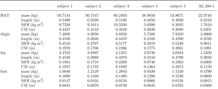
Figure 3 shows the results from the experimental measurement of stride length along with the results from the simulator. Grieve & Gear (1966), Charteris et al. (1982) and Alexander (1984) normalize stride length by stature. But since stride length is necessarily strongly influenced by leg length (see e.g.Jungers 1982) and since any flexed trunk posture may reduce biomechanically effective ‘stature’ (Alexander 1984), normalization against leg length is probably more appropriate, and is adopted here. Recalling that stride length was not itself one of the criteria optimized there is good agreement between the experimental and simulation data over the full range of simulated speeds, although the simulator consistently overestimates the stride length for a given speed (or conversely under-estimates the speed for a given stride length).
Figure 4 shows the results from the A. afarensis simulation, and includes for comparison cost of locomotion data for young children (of similar body size to AL 288-1) taken from the literature (Heglund & Schepens 2003). Once again the simulator produces values which are reasonably faithful estimates of the experimental net cost of locomotion. The simulated speed range 0.6–1.3 m sK1is certainly consistent with allometrically predicted values for walking in animals between 9 and 25 kg. (cf.Heglund & Taylor 1988). In order to estimate the gross cost of locomotion we need to estimate the cost of standing in A. afarensis. The power cost of standing with straight knees for 5–6 year
old children is 3.08 W kgK1 and for 7–8 year olds is 3.02 W kgK1(Heglund & Schepens 2003) so a value of 3.05 W kgK1 was used to calculate the gross cost of locomotion from the simulator.
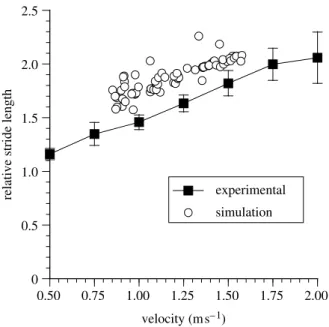
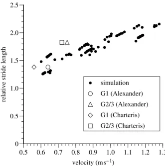
Figure 5 shows the relationship between walking speed and stride length for the simulator. We have added relative stride length information which may pertain directly to A. afarensis, derived from the 3.5 to 3.8 million year old footprint trails at Laetoli, Tanzania, plotted against velocities estimated by
Charteris et al. (1982) and Alexander (1984). We have not included the site A trail because of its uncertain affinity (Robbins 1987). The simulator predicts walking speeds of approximately 0.65–0.7 m sK1 for trail G1, and 0.95–1.0 m sK1 for trail G2/3. Since for our human subjects the simulator consistently underestimated speeds in comparison to speeds experimentally recorded for given stride lengths, it is quite possible that the A. afarensis simulation also underestimates speed for given stride lengths: actual speeds might have been still higher.
4. DISCUSSION
The predicted metabolic energy costs for the adult humans match the experimental data surprisingly well, although a perfect match has not yet been achieved. It has to be remembered that the predictions made by the
0 0.5 1.0 1.5 2.0 2.5 0.50 0.75 1.00 1.25 1.50 1.75 2.00
relative stride length
velocity (m s– 1)
experimental simulation
Figure 3. The relative stride length values obtained for the five experimental subjects and for the simulator. The error bars represent the 95% confidence limits of the mean. Note that the relative stride length is calculated by dividing the actual stride length by the total leg length (the sum of the thigh and leg segments).
0 1 2 3 4 5 6 7 8 0.50 0.75 1.00 1.25 1.50 1.75 2.00 cost of locomotion (J kg –1 m –1 ) velocity (m s– 1) 5-6 years gross 7-8 years gross 5-6 years net 7-8 years net simulation gross simulation net
Figure 4. The cost of locomotion for the A. afarensis simulator. For comparison the graph also shows the exper-imentally derived cost of locomotion for modern human children of similar body mass and stature to A. afarensis
simulator do not exactly correspond to either the net or the gross cost of locomotion as measured experimen-tally. The experimentally determined gross cost of locomotion also includes energy costs not associated with the musculoskeletal system (such as by the liver, brain, etc.) and will therefore always be considerably greater than the costs estimated by the simulator. Calculation of net cost does correct for this while at rest. However, some of non-musculoskeletal costs are dependent on locomotor speed (those of the circulatory and respiratory systems for example) so that the correction becomes inaccurate at higher speeds. In addition the net cost of locomotion also subtracts the purely postural costs of the musculoskeletal system. Whilst this is mostly desirable since the model does not include the muscles acting in a primarily postural role, such as the axial musculature, some of the muscles it does include also have a postural cost at rest. There is currently no experimental way of estimating what the simulation actually predicts: the metabolic cost associ-ated with the pattern of activation of the locomotor muscles alone.
In addition the model does not include many of the energy-saving features of the human locomotor system, in part because it is limited to two dimensions. There are no two-joint muscles to help energy transfer, and the spring mechanisms are limited to the tendons and the passive elasticity of the muscles. Storage of spring energy in ligaments is not included, and the choice of spring constant for the existing elements has not been optimized to maximize energy return. It is therefore not surprising that the actual metabolic costs of locomotion are somewhat lower than the values produced by the simulator. In addition the model is two-dimensional, so the costs and benefits inherent in the extra dimension
are ignored. These would become extremely important when investigating the value of particular anatomical structures and innovations since with a three-dimen-sional model we could, for example, investigate the effects of pelvis width independently of other morpho-logical variation.
The predicted costs of locomotion: 7.0 J kgK1mK1 (2.0 J kgK1mK1 net) for the lowest speeds, falling to 5.8 J kgK1mK1at 1.0 m sK1(2.9 J kgK1mK1net) and rising to 6.2 J kgK1mK1 (3.8 J kgK1mK1 net) at the maximum walking speeds achieved, are consistent with those we have previously published for single speeds (Sellers et al. 2004) even though we are using a completely different muscle model in this simulation. They are also consistent with the metabolic cost predicted by the only fully three-dimensional simu-lation (Nagano et al. 2005): 7.7 J kgK1mK1. Nagano and colleagues’ value includes an estimate for non-locomotor metabolic costs, and so directly represents the gross metabolic costs of locomotion. However, it should be noted that their cost estimate is for a speed of only 0.615 m sK1, at the bottom end of our range of speeds. Our gross cost is also in good agreement with experimental values for children (figure 4).
All other things being equal, our data suggest that 1.0 m sK1 was the optimal walking speed for A. afarensis. However, the optimal speed depends on the degree of time pressure on the animal—an animal with plenty of free time will actually use less energy over an extended time period by travelling at speeds which incur costs approaching the minimum of the net costs of locomotion (Sellers et al. 2004). Of course it is seldom the case that an animal is under no time constraint: higher speeds will often be adopted.
Our model predicts walking speeds for the two Laetoli trackways which were unequivocally made by human relatives, G1 and G2/3, of approximately 0.7 and 1.0 m sK1 respectively. These estimates substan-tially exceed the estimate of Charteris et al. (1982), based on relationships between stride length and speed in human adults and children (Grieve & Gear 1966): 0.56 m sK1for trail G1, and 0.72 m sK1for trail G2/3. They also exceed, to a lesser degree,Alexander’s (1984)
estimates, using dynamic scaling, of 0.64 m sK1for G1 and 0.75 m sK1for G2/3. G-2/3 consists of overlapping trails most likely made by two adults of A. afarensis. When compared to our predictions for the relationship of stride length, speed and metabolic costs, the predicted speed for G2/3 suggests that the makers were walking at, or near, their energetically optimum speed. Further, they were walking well within the range of predicted speeds for an animal of equivalent body size (cf. Heglund & Taylor 1988). Modern humans commonly adopt walking speeds between 1.0 and 1.7 m sK1, depending on the situation (Bornstein & Bornstein 1976). Wirtz & Ries (1992) note, however, that young adults most commonly choose to walk at 1.5 m sK1; this is near the energetically optimum speed we recorded for our young adult human subjects. Our estimate for A. afarensis is nevertheless, although slow compared to a young adult human, within the range of absolute values for humans, despite a short stature of about 1.1 m. Thus, our model offers further evidence
0 0.5 1.0 1.5 2.0 2.5 0.5 0.6 0.7 0.8 0.9 1.0 1.1 1.2 1.3
relative stride length
velocity (m s– 1) simulation G1 (Alexander) G2/3 (Alexander) G1 (Charteris) G2/3 (Charteris)
Figure 5. Open markers: estimated velocities plotted against Laetoli stride lengths for trails G1 and G2/3 as calculated by Alexander (1984) andCharteris et al. (1982). Solid circles: stride length and speed predictions from the A. afarensis simulator. The trend of the points, whilst largely in agreement with Alexander’s G1 value clearly predicts higher velocities for the relative stride length of the G2/3 trails.
that A. afarensis was a fully competent biped. This contrasts dramatically with Hunt’s (1994) suggestion that A. afarensis’ gait would have been ‘bipedal shuffling’. It also necessarily casts doubt on his conclusion that A. afarensis was a ‘postural biped’ with a bipedal gait compromised by the competing needs of terrestrial bipedality and arboreal climbing.
Some caution must be expressed, since uncertainties with respect to dimensions of A. afarensis apply to the present study as much as to previous studies, and our predicted velocities must therefore be regarded as very approximate values. Nevertheless, any error may actually be in underestimation, as the model of our human subjects predicted velocities consistently lower than experimentally recorded.
Although chimpanzees may possibly not have particularly short strides compared to Homo or Australopithecus (Alexander 1984) it is extremely doubtful that in bipedal gait they could sustain a similar velocity to either genus. The single extant study of metabolic costs in bipedalism (Taylor & Rowntree 1973) shows an intercept and slope much greater even than that of humans imitating chimpanzee-like (BHBK) gait (Carey & Crompton 2005). Even the normal quadrupedal locomotion of chimpanzees is expensive compared that of other mammals (Taylor & Rowntree 1973). Assuming that chimpanzees tend to walk quadrupedally at their most efficient speed, not even male chimpanzees, which tend to walk at about 0.88 m sK1 (Pontzer & Wrangham 2004), match the optimum performance predicted for bipedalism of A. afarensis: an even more marked gap exists if we consider instead female chimpanzees (0.78 m sK1).
Thus, within the limits of our model, and assuming thatTaylor & Rowntree’s (1973)data are reliable, the bipedal performance of Australopithecus afarensis, as predicted by our model is not only much closer to that of modern humans than to that of bipedally walking great apes, but at normal walking speeds, shows a clear speed/cost advantage over chimpanzee quadrupedal-ism. Climbing remains significantly more energetically expensive than terrestrial quadrupedalism for chim-panzees, despite their musculoskeletal adaptations (Pontzer & Wrangham 2004). Pontzer & Wrangham (2004) have shown that the costs of locomotion in chimpanzees are nevertheless dominated by terrestrial walking, because of very high daily travel distances, versus only limited use of climbing. If we make the major (and quite likely incorrect) assumption that the African apes existing at the time of A. afarensis were ecologically, morphologically and physiologically simi-lar to modern common chimpanzees, then our data would tend to support Rodman & McHenry’s (1980)
argument that the adoption of bipedalism offered energetic advantages to early human ancestors.
However, the advantage to chimpanzees of increased capabilities in arboreal climbing must be taken into consideration, and chimpanzees can certainly achieve speeds in quadrupedal locomotion well in excess of the maximum speed achieved by our simulation of alism in A. afarensis. Unfortunately, voluntary biped-alism is a rare event in other great apes, and the measures needed to assess its physiology usually
impossible if not unethical, so we are unlikely to be able to make a direct assessment of the physiological reasons for the gulf between bipedal performance of living apes, and that of humans, and, which is more to the point, their fossil relatives. A modelling approach similar to the present one is probably our best available tool.
Adoption of habitual, efficient bipedalism would be expected to exert an immediate influence on ranging behaviour and time budgets. Studies of modern human bipedalism and bipedalism in non-human primates can be used to quantify its consequences for time and energy budgets (for a detailed review seeSchmitt 2003). But extension of these data to early human ancestors and their relatives is problematical. As we have seen the earliest unquestionable bipeds (e.g. A. afarensis) were little more than half the mass of modern human adults. Current approaches (e.g.Pontzer & Wrangham 2004) therefore use allometric scaling equations to assign costs to locomotor activities, but even these are subject to errors relating to differences in body proportions which outside genus Homo may be quite large. However, if the nature and scale of these differences could be understood, simulation approaches using agent-based modelling, a technique from computer science which focuses on behaviour of the individual, and variation within a population, as agents move through simulated environments are very promising future possibilities.
5. CONCLUSION
Assuming that the early human relative A. afarensis was the maker of the Laetoli footprint trails G1 and G2/3, our study suggests that, by 3.5 million years ago, some at least of our early relatives, despite small stature, could sustain efficient bipedal walking at absolute speeds within the range shown by modern humans.
The predicted velocity of walking of the adults which made Trail G2/3, 1.0 m sK1, is close to the predicted energetic optimum for this species, but less than the energetic optimum for our human subjects (ca 1.5 m sK1). It is also less than the maximum velocity achieved by our A. afarensis simulations (ca 1.2 m sK1). It is however greater than the normal quadrupedal walking speed of common chimpanzees, and almost certainly represents a lower cost of transport over the same distance.
An evolutionary robotics approach can thus provide a relatively complete assessment of walking behaviour of fossil species such as A. afarensis, and may suggest its possible advantages over gaits of living non-human primates. However, our model still overestimates costs, in part because its two-dimensional nature limits it to a relatively rigid ‘compass gait’, and tends to under-estimate speed. Our present model does not encompass the detail of foot anatomy which would be necessary to investigate running and cannot accurately mimic the force production capabilities of the human forefoot. This may be why the model tends to switch to running at relatively slow speeds (1.3 m sK1(AL 288-1 model) or 1.5 m sK1(human model)—human subjects both in
our experiments and as found by others tend to prefer to run at speeds in excess of 2.0 m sK1 (e.g.
Thorstensson & Roberthson 1987;Minetti et al. 1994). Computational costs are still such that models such as the present one which can sui generis produce stable walking are still limited in sophistication with respect to detailed functional anatomical questions, while more biorealistic models (such as that ofNagano et al. 2005) have not achieved stability over multiple cycles, and cannot be easily used to predict vital gait parameters such as speed and stride length. The next generation of simulators, however, should be able to cope both with individual muscle recruitment and multiple bone/soft tissue interactions, and the elastic storage of energy, which will greatly aid our understanding of the evolution of the human locomotor system, particularly at or near the walk/run transition.
We thank our human subjects for their participation in the experiments, Professor Michael Day for encouraging our interest in the Laetoli footprint trails, and the very helpful and detailed comments from two anonymous referees. This work was supported by grants from The Leverhulme Trust, the Natural Environment Research Council, The Biotechnology and Biological Sciences Research Council and the Engineering and Physics Research Council.
REFERENCES
Aiello, L. C. & Dean, C. 1990 An introduction to human evolutionary anatomy. New York: Academic Press. Aiello, L. C. & Wheeler, P. 1995 The expensive-tissue
hypothesis: the brain and the digestive system in human and primate evolution. Curr. Anthropol. 36, 199–221. Alexander, R. M. 1984 Stride length and speed for adults,
children, and fossil hominids. Am. J. Phys. Anthropol. 63, 23–27.
Alexander, R. M. 2004 Bipedal animals, and their differences from humans. J. Anat. 204, 321–330.
Alexander, R. M. & Jayes, A. S. 1978 Vertical movements in running and walking. J. Zool. Lond. 185, 27–40.
Bornstein, M. N. & Bornstein, H. G. 1976 The pace of life. Nature 259, 557–558.
Biewener, A. A. 2003 Animal locomotion. Oxford: Oxford University Press.
Carey, T. S. & Crompton, R. H. 2005 The metabolic costs of ‘bent hip, bent knee’ walking in humans. J. Hum. Evol. 48, 25–44.
Cavagna, G. A., Heglund, N. C. & Taylor, C. R. 1977 Mechanical work in terrestrial locomotion, two basic mechanisms for minimizing energy expenditure. Am. J. Physiol. 233, R243–R261.
Charteris, J., Wall, J. C. & Nottrodt, J. W. 1982 Pliocene hominid gait: new interpretations based on available footprint data from Laetoli. Am. J. Phys. Anthropol. 58, 133–144.
Crompton, R. H., Li, Y., Wang, W., Gu¨nther, M. M. &
Savage, R. 1998 The mechanical effectiveness of erect and “bent-hip, bent-knee” bipedal walking in Australopithecus afarensis. J. Hum. Evol. 35, 55–74.
Crompton, R. H. et al. 2003 The biomechanical evolution of erect bipedality. Cour. Forsch. Inst. Senckenberg 243, 115–126.
Davis, L. 1991 Handbook of genetic algorithms. New York: Van Nostrand Reinhold.
Delp, S. L., Loan, J. P., Hoy, M. G., Zajac, F. E., Topp, E. L. & Rosen, J. M. 1990 An interactive graphics-based model of the lower extremity to study orthopaedic surgical procedures. IEEE Trans. Biomed. Eng. 37, 757–767. Featherstone, R. 1987 Robot dynamics algorithms. Boston:
Kluwer Academic Publishers.
Grieve, D. W. & Gear, R. J. 1966 The relationships between length of stride, step frequency, time of swing and speed of walking for children and adults. Ergonomics 5, 379–399. Harcourt-Smith, W. E. H. & Aiello, L. C. 2004 Fossils, feet
and the evolution of human bipedal locomotion. J. Anat. 204, 403–416.
Hay, R. L. 1987 Geology of the Laetoli area. In Laetoli: a Pliocene site in Northern Tanzania (ed. M. D. Leakey & J. M. Harris), pp. 23–47. Oxford: Oxford University Press. He, J., Levine, W. S. & Loeb, G. E. 1991 Feedback gains for correcting small perturbations to standing posture. IEEE Trans. Automat. Control 36, 322–332.
Heglund, N. C. & Taylor, C. R. 1998 Speed, stride frequency and energy cost per stride: how do they change with body size and gait? J. Exp. Biol. 138, 301–318.
Heglund, N. C. & Schepens, B. 2003 Ontogeny recapitulates phylogeny? Locomotion in children and other primitive hominids. In Vertebrate biomechanics and evolution (ed. V. L. Bels, J-P. Gasc & A. Casinos), pp. 283–295. Oxford: Bios Scientific Publishers.
Holland, J. H. 1975 Adaptation in natural and artificial systems. Ann Arbor: University of Michigan Press. Hunt, K. D. 1994 The evolution of human bipedality: ecology
and functional morphology. J. Hum. Evol. 26, 183–202. Johanson, D. C., Lovejoy, C. O., Kimbel, W. H., White, T. D.,
Ward, S. C., Bush, M. B., Latimer, B. L. & Coppens, Y. 1982 Morphology of the Pliocene partial hominid skeleton (AL 288-1) from the Hadar Formation. Ethiop. Am. J. Phys. Anthropol. 57, 403–451.
Jungers, W. L. 1982 Lucy’s limbs: skeletal allometry and locomotion in Australopithecus afarensis. Nature 297, 676–678.
Kidd, R. S. 1995 An investigation into patterns of morpho-logical variation in the proximal tarsus of selected human groups, apes and fossil: a morphometric analysis. Ph.D. thesis, The University of Western Australia, Crawley. Kramer, P. A. 1999 Modelling the locomotor energetics of
extinct hominids. J. Exp. Biol. 202, 2807–2818.
Kramer, P. A. & Eck, G. G. 2000 Locomotor energetics and leg length in hominid bipedality. J. Hum. Evol. 38, 651–666. Latimer, B. 1991 Locomotor adaptations in Australopithecus
afarensis: the issue of arboreality. In Origine(s) de la bipedie chez les Hominides (ed. Y. Coppens & B. Senut), pp. 169–176. Paris: CRNS Editions.
McMillan, S., Orin, D. E. & McGhee, R. B. 1995 DynaMechs: an object oriented software package for efficient dynamic simulation of underwater robotic vehicles. In Underwater robotic vehicles: design and control (ed. J. Yuh), pp. 73–98. Albuquerque, NM: TSI Press.
Minetti, A. E. & Alexander, R. M. 1997 A theory of metabolic costs for bipedal gaits. J. Theor. Biol. 186, 467–476. Minetti, A. E., Ardigo, L. & Saibene, F. 1994 The transition
between walking and running in humans: metabolic and mechanical aspects at different gradients. Acta Physiol. Scan. 150, 315–323.
Nagano, A. & Gerritsen, K. G. M. 2001 Effects of neuromus-cular strength training on vertical jumping performance— a computer simulation study. J. Appl. Biomech. 17, 113–128.
Nagano, A., Umberger, B. R., Marzke, M. W. & Gerritsen, K. G. M. 2005 Neuromusculoskeletal computer modeling and simulation of upright, straight-legged, bipedal locomotion
of Australopithecus afarensis (A.L. 288-1). Am. J. Phys. Anthropol. 126, 2–13.
Nolfi, S. & Floreano, D. 2000 Evolutionary robotics. Cambridge: MIT Press.
Pierrynowski, M. R. 1995 Analytical representation of muscle line of action and geometry. In Three-dimensional analysis of human movement (ed. P. Allard, I. A. F. Stokes & J-P. Blanch), pp. 215–256. Champaign, IL: Human Kinetic Publishers.
Pontzer, H. & Wrangham, R. W. 2004 Climbing and the daily energetic cost of locomotion in wild chimpanzees: impli-cations for hominoid locomotor evolution. J. Hum. Evol. 46, 317–335.
Rechenberg, I. 1965 Cybernetic solution path of an exper-imental problem. Farnborough: Royal Aircraft Establish-ment (UK), Ministry of Aviation.
Robbins, L. M. 1987 Hominid footprints from Site G. In Laetoli: a Pliocene site in Northern Tanzania (ed. M. D. Leakey & J. M. Harris), pp. 496–502. Oxford: Oxford University Press.
Rodman, P. S. & McHenry, H. M. 1980 Bioenergetics and the origin of human bipedalism. Am. J. Phys. Anthropol. 52, 103–106.
Saunders, J. B., Inman, V. T. & Eberhart, H. D. 1953 The major determinants in normal and pathological gait. J. Bone Joint Surg. 35, 543–558.
Schmitt, D. 2003 Insights into the evolution of human bipedalism from experimental studies of humans and other primates. J. Exp. Biol. 206, 1437–1448.
Sellers, W. I., Dennis, L. A. & Crompton, R. H. 2003 Predicting the metabolic energy costs of bipedalism using evolutionary robotics. J. Exp. Biol. 206, 1127–1136. Sellers, W. I., Dennis, L. A., Wang, W. & Crompton, R. H.
2004 Evaluating alternative gait strategies using evol-utionary robotics. J. Anat. 204, 343–351.
Stern, J. T. & Susman, R. L. 1983 The locomotor anatomy of Australopithecus afarensis. Am. J. Phys. Anthropol. 60, 279–317.
Taylor, C. R. & Rowntree, V. J. 1973 Running on two or four legs: which consumes more energy? Science 179, 186–187.
Thorstensson, A. & Roberthson, H. 1987 Adaptations to changing speed in human locomotion: speed of transition between walking and running. Acta Physiol. Scan. 131, 211–214.
Umberger, B. R., Gerritsen, K. G. M. & Martin, P. E. 2003 A model of human muscle energy expenditure. Comp. Methods Biomech. Biomed. Eng. 6, 99–111.
van den Bogert, A. J. 1994 Analysis and simulation of mechanical loads on the human musculoskeletal system: a methodological overview. Exerc. Sport. Sci. Rev. 22, 23–51.
van Soest, A. J. & Casius, L. J. 2003 The merits of a parallel genetic algorithm in solving hard optimization problems. J. Biomech. Eng. 125, 141–146.
Wang, W., Crompton, R. H., Carey, T. S., Gu¨nther, M. M.,
Li, Y., Savage, R. & Sellers, W. I. 2004 Comparison of inverse-dynamics musculo-skeletal models of AL 288-1 Australopithecus afarensis and KNM-WT 15000 Homo ergaster to modern humans, with implications for the evolution of bipedalism. J. Hum. Evol. 47, 453–478. Ward, C. V. 2002 Interpreting the posture and locomotion of
Australopithecus afarensis: where do we stand? Am. J. Phys. Anthropol. 119(Suppl. 35), 185–215.
Weaver, K. F., Brill, D. L. & Matternes, J. H. 1985 The search for our ancestors. Nat. Geograph. 168, 560–623.
Weir, J. B. 1949 New methods for calculating metabolic rate with special reference to protein metabolism. J. Physiol. 109, 1–9.
White, T. D. 1980 Evolutionary implications of Pliocene hominid footprints. Science 208, 1765–1766.
Winter, D. A. 1990 Biomechanics and motor control of human movement. New York: Wiley.
Wirtz, P. & Ries, G. 1992 The pace of life reanalysed: Why does walking speed of pedestrians correlate with city size? Behaviour 123, 77–83.
The electronic supplementary material is available athttp://dx.doi. org/10.1098/rsif.2005.0060 or via http://www.journals.royalsoc.ac. uk.