Character template estimation from document images and their transcriptions

Character Template Estimation from Document

Images and Their Transcriptions

by

Mauricio Lomelin Stoupignan

Submitted to the Department of Electrical Engineering and Computer

Science

in partial fulfillment of the requirements for the degrees of

BACHELOR OF SCIENCE

and

MASTER OF SCIENCE

at the

MASSACHUSETTS INSTITUTE OF TECHNOLOGY

June 1995

©

Mauricio Lomelin Stoupignan, MCMXCV. All rights reserved.

The author hereby grants to MIT permission to reproduce and

distribute publicly paper and electronic copies of this thesis document

in whole or in part, and to grant others the right to do so.

7,?

on

/

Author

...

.

...

Department of Elect cal Engineing and Computer Science

May 19, 1995

Certified by ...

Sanjoy K. Mitter

Professor of Electrical Engineering, MIT LIDS

Thesis Supervisor

Certified by ...

...

Gary E. Kopec

Member ~

9

the Research Staff, Xerox Palo Alto Research Center

\iA.

1i . A

~n

Thesis Supervisor

Accepted by .. ..

:.ASSACHUSEITS INSTITUTE D

Frederic R. Morgenthaler

Character Template Estimation from Document Images and

Their Transcriptions

by

Mauricio Lomelin Stoupignan

Submitted to the Department of Electrical Engineering and Computer Science on May 19, 1995, in partial fulfillment of the

requirements for the degrees of BACHELOR OF SCIENCE

and

MASTER OF SCIENCE

Abstract

The problem of character template estimation (CTE) refers to extracting proper models for the shapes of characters and a set of font metrics to dictate alignment between adjacent characters. This thesis develops a maximum likelihood approach to CTE for estimating bitmap templates within the framework of document image decoding (DID). An iterative procedure is developed for template estimation given a text image and a transcription of the text. The transcription and image need not be aligned nor is it necessary for the individual glyphs in the image to be segmentable prior to CTE. The proposed approach is demonstrated on text in a variety of fonts, including a scriptlike font in which adjacent characters are connected.

Thesis Supervisor: Sanjoy K. Mitter

Title: Professor of Electrical Engineering, MIT LIDS Thesis Supervisor: Gary E. Kopec

Acknowledgments

I wish to express my deepest appreciation to my advisor Gary Kopec for being a wonderful person to work with. The guidance, constant encouragement, and freedom he gave me were invaluable. I found him to be a very admirable person.

I would also like to thank Dan Bloomberg for all the help he gave me in making the theoretical aspects of this thesis a practical reality. This research was done at the Xerox Palo Alto Research Center. Thanks go to all the researchers who made my internship there very stimulating.

Special thanks go to Angie Hinrichs for venturing with me to live in San Francisco while this research was being done. It was a wonderful experience. To all my friends at MIT, I want to thank you for sharing these past five years in all the good and bad times we've had.

I dedicate this thesis to my mother Cecilia. Words cannot express my gratitude to you for everything you have done for me. You have given me the freedom to choose my own path through life, and have offered me your love and support at every step

Contents

1 Introduction 10

2 Document Image Decoding Models 13

2.1 Image Source Model ... 14

2.1.1 Sidebearing Model . . . 14

2.1.2 Stochastic Image Source ... .. 17

2.2 Channel Model . . . ... .. . . 19

2.3 Decoder Model . . . ... .. . . 21

2.4 Background Definitions ... 25

3 Character Template Estimation with Origins Known 26 3.1 Independent Maximum Likelihood Template Estimation ... 27

3.1.1 Optimize y with ao and al fixed ... 29

3.1.2 Optimize ao and al with Y fixed ... 34

3.1.3

Assumptions

. ...

. . 37

3.1.4 Convergence of Y, ao, al . . . ... . . .37

3.1.5 Experimental Results . . . ... . . . . .38

3.2 Maximum Likelihood Template Refinement ... 43

3.2.1 Cluster Likelihood ... 49

3.2.2 Assumptions .. ... 51

3.2.3 Cluster Assignment ... 52

4 Character Template Estimation Given Baselines and Transcription 65

4.1 Overview . . . . 4.2 Page Model Given Baselines and Transcription .

4.2.1 Baselines . ...

4.2.2 Line Model ...

4.2.3 Page Model Using Separable Sources 4.3 Alignment Algorithm - Modified Viterbi .... 4.4 Iterative Template Estimation Procedure Using

Modules. 4.4.1 Convergence of y ... 4.4.2 Initial Templates. 4.4.3 Setwidth Estimation. 4.4.4 Experimental Results. 4.5 LTR and RTL Decoding ...

4.5.1 Template Metric Estimation ... 4.5.2 LTR and RTL Correlation ... 4.5.3 Experimental Results.

5 Summary and Further Directions 5.1 Summary.

5.2 Further Directions ...

A Cluster Assignment Problem is NP-complete

66 66 66 69 72 74 . . . .Alignment Alignment . . . . and CTE ... . .. 78

... . .79

... . .81

... . .84

... . .85

... . . . 102 ... . . . 103 ... . . . 104 ... . . . 105 113 113 114 118

List of Figures

2-1 Communication System.

2-2 Sidebearing model for character placement. Character origins are in-dicated by crosses. (a) Character spacing and alignment parameters. (b) Example of negative sidebearings. The character bounding boxes overlap, but the character supports do not...

2-3 Greekirngs of Adobe Times-Italic. The origin and setwidth of the "j" are indicated by crosses. The gray region is the superposition of all characters from the font. (a) Right Greeking; each character is right-aligned with the origin. (b) Left Greeking; each character is left-right-aligned with the origin ...

2-4 A Simple Stochastic Image Source ... 2-5 Asymmetric Bit-Flip Noise Model ... 3-1 3-2 3-3 3-4 3-5 3-6 3-7 3-8 3-9

Maximum Likelihood Template Estimation ... Pixel Assignment Threshold Function ... Original Image ...

Character Origins ...

Extracted Instances of Character "a" ... Maximum Likelihood Estimated Templates ... Maximum Likelihood Template Reconstructed Image Cluster Cover Through Noise Model {y}--{z} . . .

Greedy CAP Algorithm . .

...

3-10 Maximum Likelihood Templates Through Greedy Algorithm

13 15

... . .16

. ... .. .. .. .. . . .17 . . . .20 28 . . .. . . . .. 31 40 . . . .. . . 40 . A. . . .

e

41 . . . 42 . . . .. 43 . . . 50 . . . 53 54

3-11 Greedy Template Reconstructed Image ... . ... 55

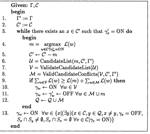
3-12 Local Search Algorithm for Greedy Solution . ... 58

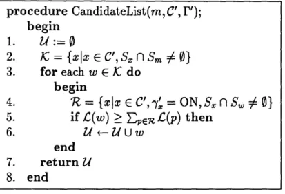
3-13 Procedure CandidateList(m, C',r) ... 59

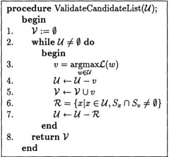
3-14 Procedure ValidateCandidateList(U) ... . 60

3-15 Procedure ValidCandidateConflicts(V,C',r') ... 61

3-16 Greedy Templates After Refinement . ... 62

3-17 Refined Template Reconstructed Image ... 63

4-1 Baseline and Endpoint Vectors on Image Plane . ... 69

4-2 Line Model ... 71

4-3 Page Model Given Baselines and Transcription . ... 73

4-4 Alignment Algorithm - Modified Viterbi . ... 76

4-5 Typed Document Estimated Baselines . ... 77

4-6 Template Estimation Procedure Using Alignment and CTE Modules. 78 4-7 Template Image Canvass. (a) Local Coordinate System. (b) Initial Template. Origin is indicated by a cross, initial setwidth vector is 0o. 8 1 4-8 Invalid Alignment Using Templates with Arbitrary Image Positions. (a) Character images arbitrarily positioned with respect to origin. (b) Observed textline image. (c) High scoring alignment of templates on

textline

image.

...

....

...

83

4-9 Typed Document Initial Templates . ... 88

4-10 Typed Document Estimated Templates after 4 Iterations ... 89

4-11 Typed Document Template Reconstructed Image after 4 Iterations 90 4-12 Old English Original Document . ... . . 91

4-13 Old English Document Estimated Baselines . ... 92

4-14 Old English Document Initial Templates ... 93

4-15 Old English Document Greedy Templates after 10 Iterations ... 94

4-16 Old English Document Refined Templates after 10 Iterations ... 95

4-17 Old English Template Reconstructed Image after 10 Iterations ... . 96

4-19 Mistral Document Estimated Baselines ... 98 4-20 Mistral Document Initial Templates ... 99 4-21 Mistral Document Estimated Templates after 8 Iterations ... 100 4-22 Mistral Document Template Reconstructed Image after 8 Iterations 101 4-23 Metric Estimation on Aligned Characters. Estimated origins are

indi-cated by solid crosses. True origins are indiindi-cated by dotted crosses. . 103 4-24 Alignment of LTR and RTL templates . ... 105 4-25 Mistral Document LTR Templates after 6 Iterations ... 107 4-26 Mistral Document RTL Templates after 6 Iterations ... 108 4-27 Mistral Document Correlated LTR Templates after 6 Iterations . . . 109 4-28 Mistral Document Correlated RTL Templates after 6 Iterations . . . 110 4-29 Mistral Document LTR Templates after 8 Iterations ... 111 4-30 Mistral Document Template Reconstructed Image after 8 Iterations . 112 A-1 CAP Construction from Minimum Cover ... 121

Chapter 1

Introduction

Character recognition is an area of pattern recognition that has received much atten-tion with an increase in demand for automated processes that convert printed docu-ments to electronic docudocu-ments. Two major techniques used in character recognition are feature extraction and bitmap template matching. Feature extraction strategies start with a test pattern and measure a number of features that are known, in ad-vance, to be good descriptors for the pattern. Template matching strategies compare the test pattern with stored reference patterns.

Template based modern Optical Character Recognition (OCR) systems face the problem of decoding the degraded image of a document accurately. These systems rely on knowledge of what each character looks like, and perform recognition through pattern matching across the image.

One problem with OCR systems of this type is that they are not capable of maintaining high OCR accuracy across a heterogeneous document collection. One key observation is that image quality is likely to be relatively uniform across the pages of a single document, reflecting constancy in the physical degradation process involved. The concern is that the character template models used by an OCR system are a reflection of what an ideal character looks like, and might not be well suited to recognize document images where each observed instance of a character has been similarly degraded. One proposed solution is to adapt the character templates by training them on a set of sample images and the corresponding transcriptions so that

the new templates are able to more accurately recognize similar images.

In other situations we sometimes find document images for which we do not have models for the shapes of the characters that comprise it, but for which we would like to recongize a large number of images. One solution to this problem is to manually

draw each character model. This would be a very tedious enterprise, the models would have to be drawn to represent the observed image in some optimal sense (by hand this would probably be how well the character templates look), and would probably suffer from inaccuracies introduced by the artist. Another solution is to segment a sample image, label individual glyphs using the corresponding transcription of that imrnage, and train the character templates as before. This is tedious and sometimes error prone on images having a lot of blur, or non-segmentable text like arabic or musical scores.

This thesis addresses the two related character template estimation (CTE) prob-lems. In the first problem, suppose one is given a possibly non-perfect transcription, a degraded document image, and an alignment of the transcription to the image con-sisting of a set of glyph label, glyph position pairs. The problem consists of estimating the bitmap character templates that were used to create the image. This problem dliffers from the classical simple estimation problem of fitting a character template tLo a set of observed character images in that we do not have isolated characters. Rather we know only the location of each character origin, but do not know which of the pixels in the vicinity of the origin belong to the character and which belong to neighboring characters.

The second problem we address is a generalization of the first; we are now only given a document image, a transcription of each text line in the image and the vertical position of each text line baseline. Unlike the first problem, we are not given the horizontal positions of the characters in a line; the transcription gives an ordered sequence of observed characters but not their exact locations.

A desirable characteristic of any approach to character template estimation is that it be based on strong theoretical foundations. This will give us several advantages over ad-hoc (hand-tuned) procedures. First, we will be able to justify our procedures

on theoretical analyses rather than just on empirical results. Second, we will be able to extend the results to a general class of images that follow an assumed model of document generation. Third, we will be able to provide an explicit measure of optimality to the problem against which we can measure our success.

This research develops an approach to CTE within the framework developed by the document image decoding group (DID) at the Xerox Palo Alto Research Center [11]. The DID approach models document generation and decoding in terms of classical communication theory, where every stage of the process is explicitly modeled using detection and estimation theory, language formalisms, and adherence to statistical and probabilistic principles.

In the DID model, an ideal document image is generated from a set of ideal char-acter templates by "painting" these templates on an image canvass in some logical arrangement. The document is then degraded through printing, handling, and scan-ning, which introduces distortions such as stains, skew, blurring, thinscan-ning, stretching, pen marks, and other similar alterations. Finally, the observed document is decoded by generating the most likely original clean image making explicit reference to the imaging procedure and noise model.

The rest of this thesis is organized as follows. Chapter 2 presents the theoretical framework of document image decoding and establishes the basic definitions and notation that will be used throughout this thesis. Chapter 3 formalizes the problem of character template estimation given labeled origins on a document image and shows that it is an NP-complete problem. This chapter also provides a suite of algorithms designed to efficiently estimate a set of templates, and evaluates their performance experimentally. Chapter 4 formalizes the problem of character template estimation given baselines and transcription only, presents an iterative approach based on the results of chapter 3 and related document recognition techniques, and evaluates the approach experimentally on different types of images. Finally, chapter 5 presents a summary and discusses future directions.

Chapter 2

Document Image Decoding Models

As an important background to this research, we first review the theoretical frame-work of document image decoding (DID) upon which this thesis is based [12, 11]. We begin with the basic communication problem provided to us by information theory, shown in figure 2--1. The DID framework casts the problem of document image

recog-lition in terms of classical communication theory, where every stage of the process shown below is explicitly modeled using detection and estimation theory, language formalisms, and adherence to statistical and probabilistic principles.

In this view, a message source randomly produces a message X; an encoder de-terministically encodes X into an ideal bitmapped image 1'; a channel randomly

degrades the ideal image Z' into an observed image I; and a decoder deterministically mraps I into a reconstructed message, or logical document structure. X.

We discuss the the main elements of this framework - source, encoder, channel, decoder - as applied to images, in the following sections.

X Z' Z

Source Encoder Channel Decoder

2.1 Image Source Model

The typestyle is a visual property of the printed output; it is not part of the doc-ument's logical structure. For this reason, the source and the encoder must be re-garded as separate modules; the source producing a message that someone is trying to communicate, and the encoder providing a model for putting that message into a bitmapped image that we see as a document.

In the framework described in [11], the message source and the encoder are merged into a single image source that simultaneously generates a message and a typographic structure. The model for the stochastic source and encoder is partly motivated by the sidebearing model of character shape and positioning [9]. In order to understand the stochastic source model and the encoder, we must first describe this document production model that is embedded within their descriptions.

2.1.1 Sidebearing Model

Character shape and positioning in digital typography is usually based on some vari-ant of the sidebearing model [9] shown in figure 2-2. This model specifies glyph align-ment parameters that specify the relative locations of the local coordinate systems of adjacent characters in a line of text.

A character template is a bitmap spanning the x-y plane with a distinguished local

origin. An instance of a character on a page is known as a character glyph. The set

of black pixel positions of a template is called the support of that template.

A set of parameters that describe the relative placement of glyphs with respect to one another are called font metrics. In this thesis, we will be primarly concerned with font metrics that determine horizontal letterspacing.

The character coordinate system is the space in which an individual character shape is defined. All metrics are interpreted in the character coordinate space. The origin of the character is the point (0,0) in the character coordinate system. The setwidth of a character Q is the vector displacement, AQ = (Ax, Ay), from the local origin of that character to the point at which the origin of the next character is

nor-d

~--w

-! X W , i~~~~ ~11 A.--I : ... ...I ... - ... (a) (b)

Figure 2-2: Sidebearing model for character placement. Character origins are in-dicated by crosses. (a) Character spacing and alignment parameters. (b) Example of negative sidebearings. The character bounding boxes overlap, but the character supports do not.

mially placed when imaging consecutive characters. Most Indo-European alphabets, including Roman, have Ax > 0 and Ay = 0; other alphabets have Ax < 0, such as Semitic, or non-zero Ay, such as Oriental.

The bounding box of a character is the smallest rectangle, oriented with the char-acter coordinate axes, that will just enclose the charchar-acter's shape. The width of a character is the corresponding width w of the bounding box. The left sidebearing is the horizontal displacement A from the origin of the character to the left edge of the bounding box. Similarly, the right sidebearing is the horizontal displacement p from the right edge of the bounding box to the origin of the next character. The depth below baseline is the vertical distance from the character origin to the bottom of the character bounding box.

The horizontal component of the setwidth is related to the sidebearings and the bounding box width by the relation

Ax = A + w + p. (2.1)

The intercharacter spacing term d is related to sidebearings by

d = pi + A (2.2)

$

+

+

0

(a) (b)

Figure 2-3: Greekings of Adobe Times-Italic. The origin and setwidth of the "j" are indicated by crosses. The gray region is the superposition of all characters from the font. (a) Right Greeking; each character is right-aligned with the origin. (b) Left Greeking; each character is left-aligned with the origin.

respectively.

Why use the sidebearing model? It provides great flexibility and can be generalized to a wide range of images. Consider a font for music notation. Musical symbols are not arranged one after the other as in text. However, by correctly specifying the font metrics for each glyph, as explained in [14], the sidebearing model is useful for describing images of music.

The design of typefaces implicitly carries with it a characteristic that will turn out to be a very important one for character template estimation, the notion of non-overlapping template supports. The non-overlapping support observation can be formalized as follows (we assume that all character images are from the same font).

Let Y E Y be a character template drawn from a set of templates y. Let Y[0o]

denote Y shifted from an arbitrary origin (0,0) so that its origin is located at o.

Define

GR=

U

Y[-Ay] (2.3)

YEY

to be the right greeking of y. Recall that the setwidth of a character Q, denoted by AQ = (Ax, Ay) is the vector displacement from the character origin to the point at which the origin of the next character is normally placed when imaging consecutive characters of a word. Loosely then, GR is the superposition of font characters aligned

(pr(t), At, Y(t))

ni

nF

0 · · · · · 0v·

t

Figure 2-4: A Simple Stochastic Image Source on the right. We can similarly define the left greeking of Y as

GL = U Y[0] (2.4)

YEY

The observation about non-overlapping support of characters may then be for-malized by the following two conditions

Y n

GR = 0, (2.5)

Y[-zyY] f GL = 0 (2.6)

for each Y E Y. This is illustrated in figure 2-3.

Although this thesis will deal mostly with documents generated using conventional letterform typography, there are extensions of this research to the analysis of images such as musical scores. Our initial approach will show that enforcing the templates to have non-overlapping supports produces visually pleasing results.

2.1.2 Stochastic Image Source

The stochastic image source is modeled by a Markov source, as shown in figure 2-4. A Markov source is a Markov chain with the additional characteristic of transitional attributes; when described as a directed graph, every transition arc t of the Markov

chain is labeled with a triple,1 _{(pr(t), At, Y(t)), where pr(t) is the transition}

proba-bility, Y(t) is a template, and At is a displacement vector. The Markov chain has a unique initial state ni, and a final trap state nF.

tem-plate associated with that transition. In our formulation, the displacement vectors associated with every transition are assumed to satisfy the requirement that the sup-ports of two consecutively imaged templates do not overlap with each other. We will also impose the general requirement that the support of any imaged template does not overlap with the support of any other template on that image.

As the chain evolves according to its transition probabilities, a path 7r through the Markov source is described as the sequence of transitions the chain takes: = t ... tp, where t is a transition out of the initial state nI. A complete path is a path for which

tp is a transition into the final trap state nF.

A complete path 7r = tl... tp through the Markov image source defines an asso-ciated document image as follows. Imagine an image automaton that begins in an initial position on the image canvass which we will take to be the upper left hand corner of that canvass.2 With each transition t, the imager takes the corresponding template Y(ti), positions the origin of the template at its current position and paints the image of that template on the canvass. It then updates its location on the canvass by the vector At,, and waits for the next transition until the Markov chain enters the final state nF, and the image has been generated. It must be noted that the template Y(ti) can be a null template, such as a carriage return or small transitions to adjust intercharacter spacing, in which case the layout information is entirely carried by Ati. The above imaging procedure can be interpreted as forming a union of templates across the canvass at given locations defined by the sequence of displacement vectors Ati; in other words, through the evolution of the Markov chain, the imager "paints" template Y(ti) on the canvass at position -1 At,. We define the sequence of posi-tions xl ... xp+l associated with each path 7r by

xl = 0 (2.7)

zi;+l

=

i

+ Ai.

(2.8)

2

This particular coordinate system uses this corner as origin, and defines positive x to the right, and positive y down.

If we define the function f : ti - {1, 2,..., T} that maps3 _{transition ti to a template}

in the set of all possible imaging templates y = {y(1),y(2),... ,y(T)}, such that Y(ti) = y(f(ti)), then the imager forms the associated document image Z' as

P

' =

U

Y(f(t"))j,]. (2.9)

i=l

The transition probabilities pr(t) of the Markov source give us a probability distri-bution on complete paths by

P

Pr(ir) = Ipr(ti). (2.10)

i=l

Under the assumption that every path produces a unique image,4 _{then Pr(Z') = Pr(ir).}

We must point out that for a given transition t, the transition probability pr(t) of the Markov source cannot be interpreted as the independent probability of the corresponding template y(f(t). In a given Markov chain, two distinct transitions with different transition probabilities might have the same template associated with them. For this model, the probability distribution of clean images is a function of the possible paths through the Markov source, and not of the imaged templates.

2.2 Channel Model

The channel introduces distortions into a document through printing, photo-copying, handling and scanning. These distortions appear to us as random noise, pen marks, stains, skew, rotations, blurring, and other similar perturbations. A noisy channel is a random system that establishes a statistical relationship between its input and its output; it's output is not completely determined by the input. Although realistic document image defect models can be very complicated, an independent, asymmetric bit-flip noise channel shown in figure 2-5 is proposed in [11] for simplicity. This choice yields very nice analytical and experimental results.

ao 0

a1

Figure 2-5: Asymmetric Bit-Flip Noise Model

In the ideal binary image ' = {yi I i E Q}, every pixel is indexed by Q. We will assume that images are rectangular so that Q is the integer lattice [0, W) x [0, H), where W and H are the image width and height, respectively. The channel maps the ideal image into an observed image I = {zi i E Q} by introducing distortions.

The asymmetric bit-flip channel is completely characterized by two numbers, al and a0, which represent the probability that each black (white) pixel in an ideal image

yi gets mapped to a black (white) pixel in the observed image zi. These parameters are assumed to be constant over the image.

With this model, the probability of an observed image I given an ideal clean image I' is simply

Pr(IZ') =

JJ

[aO-')(1

-

ao)z'](

-Yi)

O'(

[

-1

a

)(1-zi)]'.i

(2.11)

iEn

If we let O be the all-white background image, then

Pr(IlZo) =

II

a1 Z)(1 - a0)zi (2.12)

iEl

and we can normalize Pr(IlI') into a likelihood ratio form that will give us several advantages and be easier to manipulate

Pr_____ ____1-l i

a

0a1 YiZi

(

P(lZIo)

usn t

a-o(olJ

A u

We define the log normalized probability as

£(Il')

- log

Pr(II')

(2.14)

log (la(1 Y + log c)(lal)) YiZ (2.15)

iE iEQ

= 11Illog ( ) +

I

AIlg (( o)( o )) (2.16) where

II'll1

gives the number of black pixels in I', and I'A/ denotes the bitwise logical AND of images Z' and I. This log normalized probability has a very important decomposition property. If an image Y is generated as a union of templates whose support does not overlap as in (2.9), then it is easy to see that

P

£(IlI'

)

=

E

C(IY((i))[XTi]).

(2.17)

i=l

The quantity

£C(ZII')

is the lognormalized probability that describes the degree of matching between an observed image I and a template constructed image I'. In image decoding, (ZIIZ') gives a matching score for any image 2' we consider to be the original clean one that generated the observed image I through the noise channel. Equation (2.17) can be interpreted as the aggregate likelihood of every independent template that makes up the ideal image across the observed image.

We define £(.) as the likelihood function of its argument. This notation will be used extensively to refer to likelihood, and its use will be aparent from context.

2.3 Decoder Model

The decoder takes as input a noisy version of the original image and tries to invert the effects of the encoder and noisy channel. The decoder can then output a re-constructed image, a transcription of the document image, or some other structural information about the document. The decoder must, therefore, incorporate within itself knowledge of the source and channel models.

image that could account for the observed output image. There is not a one-to-one correspondence between every input and every output. Instead, there exists a prob-ability distribution between an observed noisy image and every possible clean image that could have been constructed using the source model. For example, although an all-white image could have generated an observed document through the noise channel, this is a highly improbable event. Intuitively, the image that has the high-est number of matching symbols will be the one that generated the document.5 We formalize our intuition by reverting to decision theory.

Given the finite set of templates and the document production rules embedded in the source model, there is only a finite sample space of clean images that the source model can generate on the image canvass, I, X,..., . Furthermore, given the complete description of the Markov source model, we can also associate an a-priori probability to each sample in the space of clean images, Pr(Z;'), as shown in section 2.1.

Now, given the noise model and all possible clean images, we can associate a probability to the event that the observed noisy image was generated from a given

clean image, Pr(ZIZT), as shown in section 2.2.

All the decoder has to do now is to decide on the "best" clean image. Let us generalize and assume that we have a set of costs, Cij, of deciding I' as the original image when the true original image is 2j. We must now specify a decision rule for the decoder to choose one of the n clean images based on the observed image I, such that the expected cost of choosing the wrong image is minimized. This is exactly the M-ary hypothesis testing problem, where we have:

* M hypotheses 2, I,...,

IM

with a-priori probabilities Pr(I').

· A set of costs, Cij, of deciding I7 when 7j is true.

* The set of distributions Pr(1j4IJ) of our observation given that each of the hy-potheses is correct.

If the set of costs have the form Cij = 1 - j, then it is well-known [21] that the optimal decision rule is the maximum a-posteriori (MAP) rule,

I'

= argmaxPr(I'lI) (2.18)

I'

= argmax Pr(IL') Pr(I') (2.19)

z' Pr(7)

= argmax Pr(ZI') Pr(I') (2.20)

I'

We can normalize Pr(ZI1') above by Pr(ZIIo) since it does not depend on I', and from the monotonicity of the logarithm, we can also maximize the logarithm of the resulting function,

2Z' = argmaxlog Pr(lT2') Pr(I') (2.21)

z,

Pr(IIo)

= argmax [log PIr(JI') + log Pr(I')] (2.22) = argmax [(IlI') + log Pr(Z')] (2.23)

I'

argmax

{

[c£(IY((ti))[i]) + log pr(ti)]

}

(2.24)

where the last equality used the results from section 2.2. Under the assumption that every clean image 2I' is produced by a unique path 7r through the image source, we can equivalently talk about the path through the source that optimally represents the observed image in the MAP sense.

X = argmax£(Z, r) (2.25)

7r

argmax [(IZI') + log Pr(T)] (2.26)

7r

argmax I [C(I

jY(f(ti))[i])

+ logpr(ti)]

}

(2.27) 3Both approaches can be interpreted as a maximization of the likelihood of the observed image given a clean image and the a-priori probability that this clean image came from the markov source. MAP decoding tries to find a clean template reconstructed

so that in the MAP sense, this template reconstructed image is the original image. MAP decoding of an observed image I with respect to a given image source involves finding a complete path r through that source which maximizes L(1, 7r) over all complete paths through the Markov source. In [11] it is shown that MAP decoding can be reduced to solving the following recurrence relation

(n, x)

= tlvax {L(V,

x-

At) + (I Y(](t))[ ) +

log

pr(t)}

(2.28)

where n and v are variables representing states in the Markov source and t represents a transition into state n. The maximization in (2.28) can be computed using a dynamic programming algorithm called a Viterbi algorithm.

The recurrence term £(n, x) gives the best likelihood score if a path through the source had gone through state n at a position in the image plane during the generation of the clean image. The main recurrence arises from the fact that to go through (n, x) while generating the image, the previous stage must have been (v, 7-At), for some transition t going from v to n. The first term in the sum, C(v, 7- At) accounts for the a-posteriori probability of reaching the previous stage (v,x- - t), the second term £(IY(f(t))[ -iAt]) gives a matching score for the template y(f(t)) at location (- At) on the observed image, and the last term log pr(t) accounts for the a-priori probability of continuing this path by taking transition t. The maximization in this recursion gives the best path through the source of reaching (n, x) from among all the possible previous states.

By performing this maximization for each node n and image position x, the result is a complete path through the source that maximizes the matching score between all of the imaged templates through that path,

L

P 1 (12IY(f(t))[xi]) =

£(I1I'),

and the a-priori probability of that path, Pi=l logpr(ti) = log Pr(7r).

2.4 Background Definitions

In this section we give a few basic definitions that will help establish consistent no-tation throughout the rest of this thesis.

y(i) will denote the ith labeled character template. This can be a normal printing character, a space character, or a null template.

y = {y(1) y(2) ., ,y(T)} will denote the set of all character templates used to generate the observed image.

I will be the observed image.

7r will be a complete path through an image source.

= U!= Y(f(ti))[xi] will denote the template reconstructed image given the path through a stochastic image source and the set of imaged characters y. The operator II

QII

gives the number of black pixels in Q. The argument Q can be an image or a vector of image pixels.

The operator IQI gives the total number of pixels in an image Q, or the number of elements in a set Q. If Q is a collection of sets, the operator gives the number of sets in Q.

X A W denotes the bitwise logical AND of images X and W.

(-Q) denotes the inverse of an image Q, i.e. bitwise complement.

Zj will denote the jth observed instance of a character. This image may or may not be that of an isolated character.

Z =

{

Z₁, 72,.. ., ZN} denotes the set of observed instances of a given character.

£(.) is a likelihood function. Its specific definition will be aparent from context. The assignment operator A - B evaluates B first and assigns the result to A.

Chapter 3

Character Template Estimation

with Origins Known

Using the models and notation reviewed in the previous chapter, we pose the first problem. Given a complete path r0o = t,...,tp, a mapping function f : ti

{1,...,T}, the set of displacement vectors Ati, and the observed document image I generated by this path, the question is how to determine the set of templates

y

=

{y(l),y(

2

),...,y(T)}

that optimally

represent

the observed

image

I. This

problem is equivalent to saying that we are given the origin of every glyph on the document image, a label on each origin, and we are trying to determine the image of the templates corresponding to each label.

Using the results of section 2.3, this quantitatively translates to finding the set of templates y that maximizes the likelihood of the observed image given the template reconstructed image,

P

argmax

£(I[I')

= argmax

E

£(I

Y(f(t'))[Xi]).

(3.1)

I' 2' i=1

This problem would be very easy if we were given the isolated observed instances of every given character. The variable to be estimated would be the original character template, Y, and the measurements of this template would be all the isolated observed instances of that character, Z. Estimation theory would now dictate that the best

estimate of that template is given to us by the Maximum Likelihood estimator Y = maxy Pr{Z I Y}.

This "best" estimate of each individual template also maximizes L(ZIZ'). Simply note that the terms in the sum on equation (3.1) can be re-grouped into classes corresponding to the likelihood of a given template given all of its observed images. Maximizing each one of these classes individually maximizes the sum of the classes, and consequently

£C(IT').

Unfortunately, given a document image with character origins, there is no in-formation about the locality of the character glyphs with respect to this origin. In addition, any local region about this origin may contain pixels belonging to the de-sired character and extraneous pixels belonging to other glyphs in the vicinity of the origin. This problem differs from the classical simple estimation problem of fitting a character template to a set of observed character images in that we do not have isolated characters. Rather we know only the location of each character origin, but do not know which of the pixels in the vicinity of the origin belong to the character and which belong to neighboring characters.

We will tackle this problem as follows. We will obtain the observed instances of every character by extracting a fixed size region of image about each of the labeled character origins on the image. We will treat this set of character images as a set of isolated characters and perform the optimization described above. The resulting set of templates will contain a lot of noise, mainly because the observed instances for each character are not isolated characters. We will then proceed to "clean" these templates by enforcing the disjoint template support requirement.

3.1 Independent Maximum Likelihood Template

Estimation

In Maximum Likelihood Estimation, we assume that the variable to be estimated is unknown. Furthermore, we assume that we have a probabilistic model of the

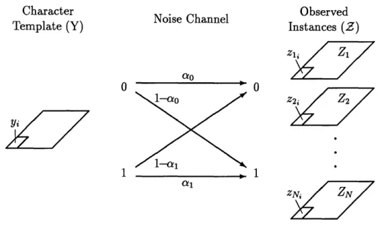
relation-Character Observed Noise Channel

Template (Y) Instances (Z)

0 ~ 0 o 0t _z 2 2•1117i~~ ~ Yi / 7~~~~~~~~~~~~~. I _ I a1 ZNi/ X 7

Figure 3-1: Maximum Likelihood Template Estimation

ship between the variable to be estimated, Y, and its measurements, Z. Maximum Likelihood then tells us to take as an estimate of Y the value that makes its actually observed values of Z as likely as possible. That is,

Y = max Pr {Z]Y}. (3.2)

Y

Figure 3.1 illustrates the ML template estimation scenario. The observed in-stances of a character, Z = {Z1, Z2,..., ZN}, are obtained by extracting a fixed size

image region about each of the labeled origins of that character. We will assume the extracted glyphs are rectangular with width Wo and height Ho so that 5 is the integer lattice [0, Wo) x [0, Ho), and in each binary image, Zj = {zIj, i E 5}, every pixel is indexed by .

Let us denote the ith indexed pixel of template Y by yi. Through the noise channel, this pixel maps to the ith indexed pixel in every observed instance. We will define the observed data vector of yi as Zi = {zli, z₂,..., zN }. The probability of Zi

given the source pixel yi and the noise model parameters ao and al is

Pr

{zi

i, ao, al}

=

I

[ )

o)Zj'

₎ (

[al

_{. (3.3)}

j=]

Assuming pixels are independent of each other, we can write the probability of the observed images given their template and the channel parameters as

Pr{Z I Y,ao, al} =

II

Pr{Zi I

i,

ao,

a}

(3.4)

iEg

I=

I

[l-ZI)(1

'I

- o)ZJi]

[a(1l-

l)(1-zi)]

i

_(3.5)

iEQ j=1

Substituting (3.5) into (3.2) we write the Maximum Likelihood decision rule as

ax

II

i) )ji(1 ao) [a" - Cil)(lzi)]Y (3.6) ,iE j=l

This maximization cannot be performed analytically, but can be done iteratively via a gradient search. Specifically, starting with arbitrary values for a0o and al, we

obtain a new template Y' by maximizing (3.6) for Y using fixed values of a0 and al;

then we update the channel parameters by maximizing (3.6) for a0o and a using Y'.

This procedure is repeated until we converge to some local maximum. The following two sections derive the maximizing values for Y, ao, and a at every iteration, and derive a test to assess convergence of this procedure.

3.1.1 Optimize y with ao and al fixed

Given the observed set of images Z = {Z1, Z2,... , ZN} of a template Y, our objective

is to decide whether to assign a value of 0 or 1 to every pixel yi in Y. Since y E {0, 1}), we have a binary hypothesis testing problem and the ML decision rule is

Yi=O

Pr{Zi I yi = O,oao, i} < Pr {Zi yi = 1, ao, a1}. (3.7)

Setting Yi = 0 and Yi = 1 in (3.3) we have

H

1 -(1z)(ao)zi, j=l Yi=O- N Yi=1 j=1 Yi=O Yi=1

(1 -

al)(

-z ji) 1.

Taking logarithms and noting that

ZE}=1

zji = IIZill, we rewrite (3.9) as Nlog ( ao) + IlZilllog _{Val ~} ((1-ao)(1-l))_{~~ aoa~l}

Yi=O

> 0.

yi=l

(3.10)

We must be careful of the values of each of the log terms. There are two regions of values for the a's to consider:

* a1 > 1 - aO.

In this case, log ( )

decision rule as follows

> O and log ((1-o)(1-al))

_\ia

_{) < 0}

< We rewrite the ML

Yi =O

yi=1

yil log

o(

)ao < log ( oal

Yi=o log (1-ao)(1-aj))

* a1 < 1 - ao.

In this case, log (-al) < 0 and log ((1-o)(1- 1 )) > 0.

decision rule as follows

I1 11

N

Yi =O yi=l yi=O < Yi--We rewrite the ML Nlog ( ao) log (1-al) (3.13) (3.14)

log

(

_aoal

₎

k (1-o) (1--aj))] Nr 1 o ) ((1 - )( 1- ) j i

j Vlal

aoal

j=1 (3.8) (3.9)

-A1 l llog (1_1o)(1jlO))

IIzi 11

N

(3.11)

(3.12)

0

0 1

Figure 3-2: Pixel Assignment Threshold Function

In both cases, we find the same threshold on the number of black pixels that must be present at each position i in the observed images, but with different hypotheses deciding whether the template should have that pixel assigned to black or white. In the region ac > 1 - co, foreground pixels are more likely to be observed as black than background pixels, which is the normal case. In the region al < 1 - c0, background

pixels are more likely to be observed as black than foreground pixels, and the channel can be interpreted as producing "reverse video". Figure 3-2 shows a plot of this threshold as a function of the channel parameters.

One of the interesting things to point out from the analytical expressions and plot of the threshold function is that there are four regions of interest:

I a > 1 - cao and ao < al.

This is the "normal" case where the threshold sets the minimum fraction of black pixels that must be present in the observed data vector to decide that the associated template pixel is black. The threshold is strictly greater than 1'

In this region foreground pixels are more likely to be observed as black than background pixels. Since ca > , the channel has a tendency to conserve black pixels. With no restriction on ao, except that ao < acl, there can be a large added contribution to the observation of black from background pixels if 1 - a > . This possibility is accounted for by having a large threshold.

II a > 1 - ao and ao > a.

This is the "normal" case where the threshold sets the minimum fraction of black pixels that must be present in the observed data vector to decide that the associated template pixel is black. The threshold is strictly less than 1

In this region foreground pixels are more likely to be observed as black than background pixels. Since ao > the channel has a tendency to conserve background pixels, which means that the observed black pixels more likely came from foreground pixels only, and since there is little contribution to black from background pixels, this explains the low threshold.

III a1 < I - ao and ao < a1.

This is the "reverse video" case where the threshold sets the minimum fraction of black pixels that must be present in the observed data vector to decide that the associated template pixel is white. The threshold is strictly greater than 12

In this region background pixels are more likely to be observed as black than foreground pixels. Since 1 - ao > , the channel has a tendency to flip back-ground pixels. With no restriction on a1, except that ac1 > ao0, there can be

a large added contribution to the observation of black pixels from foreground pixels if a > . This possibility is accounted for by having a large threshold.

IV al < 1 - ao and ao > a1.

This is the "reverse video" case where the threshold sets the minimum fraction of black pixels that must be present in the observed data vector to decide that

In this region background pixels are more likely to be observed as black than foreground pixels. Since al < -, the channel has a tendency to flip foreground pixels, which means that the observed black pixels more likely came from back-ground pixels only, and since there is little contribution to the black from fore-ground pixels, this explains the low threshold.

In the case of cao = l, the threshold becomes , which is what one would expect since both hypotheses are equally likely. It is also interesting to note that the analysis carried out on regions III and IV would be the same as that of regions I and II if the hypotheses were switched and the threshold was compared to the fraction of white pixels in the observed data vector Zi instead.

We define the number of matching pixels ®Ei = Ej=l Zj, and the number of mis-matching pixels Ai _ N - N 1= zji, so that i and Ai are the number of pixels that

are ON and OFF, respectively, in the observed image vector Zi. We can alternatively

write the ML decision rule (3.10) as follows

Yi=O

(Ai +

i)log

(g) + Olog ((1-Co)(1- c l)) > 0 (3.15)

i=l

Yi=O

, + i)log (laC)- ilog( ceocl > 0 (3.16)

yi=

yi=l

E) log (la0 -log (CIO > 0 (3.17)

Yi=O

In this last form, we interpret the formula Oilog (-0) - Ailog (ol) as the likeli-hood score of pixel yi, which we will occasionally denote by L(yi). Notice the presence of a pixel matching score Oelog (1-0) and a pixel mismatching score Ailog (io).

3Both threshold equations, (3.12) and (3.14), disguise the fact that the ML rule will only assign a pixel to template Y if its likelihood score is positive, as is explicitly shown here.

3.1.2 Optimize c0o

and a;

1

with Y fixed

Given a fixed character template Y, and its corresponding set of observed images Z {Z1, Z2, ... , ZN}, the objective is to find the channel parameters that maximize

the likelihood of Z, given by equation (3.5). We can equivalently maximize the log-likelihood of Z. After some algebra we find that

logPr {Z I Y, ao, al}

N

= log aoEo

E

(1 - i)

iEg j=l

(1 - zj,) +

N

log(1 - o)Z ( - yi)zji + iEg j=l

N

log

ca

1

E

yizji +

i6E j=l N

log(1 - a)

E

yi(1 - zji)

iE9 j=1

(3.18)

We can now derive analytical expressions that can be easily computed for the

maxi-mizing values of a0o and cl. For ao,

0 1 N

a log Pr{Z

{ YaO, al} =-E(1

daaO 0 °Ci6g j=l

t N

1

- y)( - Zi) -

_-

_{ao iE9}

E

jE

_j=l (1 - yi)Zji. (3.19)

Setting the derivative to zero we solve for the maximizing value of ao

ao _N

E9(1

ieg j=i N iE j=l -Yi)(l - Zji) + N

E(1 -yi)

iE j=1 N

E

1(-)

A(-Zj)

j=l N

E E (1

- yi)zji

ie9 j=l (3.20) N

E E

(1 - yi)( - Zi)

iEg j=l (3.21) ao = (3.22) (1 - YZ-) (I - Zji)

A subtlety with the expression for a₀ in (3.22) is that it is very sensitive to the size of the template and of the observed images. Since the expression involves operations on the inverse of the original images, we can make a0 arbitrarily close to 1 simply

by using large sized template canvasses. Through the noise channel we expect some white pixels to turn black, and cao to have a fixed value that is realistically not 1. Background noise is observed when a white pixel in the original undistorted image is mapped to a black pixel in the observed image; it originates from "white" pixels in the original document being realized as "black" in the observed image. However, this effect is only present in the the mapping of the pixels of the original document image to pixels of the observed image. The appropriate value for ao should be calculated from the discrepancies between the observed image and the original image. Given the set of templates y we generate a template reconstructed image I' to be the assumed original image, as described in section 2.1, so that

Pr { I "', a0, a} = I [ 1z')(1 -ao)zi] ( yi) [a'i(l- al)(1-zi)]Yi (3.23)

iC1

Equation (3.23) is the likelihood function of the observed image given the recon-structed image. Similarly as before, we can find the maximizing values for a0o and al

b:)y setting to zero the partial derivatives of the logarithm of this likelihood function. With some algebra, we find that

]og Pr {I I',a, a

= logaoE (1-yi)(1-zi)+

iEI2

log(1

-

ao)Z

(1 - yi)Zi +

log acE yiZi +

iEQ

log(1 - ao1) yi(l - zi). (3.24)

iEQ

maximizing values of ao and a₁. For ao,

ao

log Pr I , o, 1} = ( - )(1 - i) (1 - yi)zi. (3.25)

ad~~ao

~-

iE(

y

1 -

ao0i

Setting the derivative to zero and solving for a0 we get

E (1 -

y

i)( - zi)

ao E _(3.26)

E

(1 -

zi)

(1--

yi)zi

(3.2

iEQ iEQ E (1 - yi)(1 - zi) E iE ( (3.27)

Z(1- yi)

iEs ao ( A (3.28)

The numerator II(-')A(-ZI)l gives the number of white pixels in the recon-structed image that were realized as white pixels in the observed image. Divided by the total number of white pixels present in the reconstructed image 11(-I') , this frac-tion is the probability that a white pixel is mapped to a white pixel; the background channel parameter ao. We follow the same procedure to solve for a,

a

loIr{7 ia 1 1

- log Pr ', ao, al = E y{iI YiZi- E Yj(l -Zi). (3.29)

,al1

1 iE

1

- lien

Setting the derivative to zero we solve for the maximizing value of a1

E YiZi

aC

1 =i

1

(3.30)

E

YiZi

+

E

yi( - i)

iEQ iEQ ien (3.31) E Yi iE2Q a1 _ (3.32) llII

In the expression for c, the numerator llZ'AIll gives the number of black pixels in the assumed original image that were mapped to black pixels in the observed image. ]Divided by the total number of black pixels present in the reconstructed image 11I'11,

this fraction is the probability that a black pixel is mapped as a black pixel; the foreground channel parameter a₁.

3.1.3 Assumptions

There is one subtlety that we must pay attention to. In the calculation of the channel parameters, we made the implicit assumption that the templates in the reconstructed irnage were disjoint. This is not generally true in this case since every estimated template will contain an estimate of its character, along with extraneous information originating from other characters in the vicinity of every instance of that character. Thus, in the template reconstructed image, there will be a lot of overlapping between the support of every template. This introduces extra noise in the reconstructed image that will be reflected in low values for a₁.

3.1.4 Convergence of

Y,

ao0,

1

The goal of template estimation is to estimate a set of templates y that maximize the likelihood of the observed image given the template reconstructed image. The process we follow is an iterative one where we switch back and forth between maximizing for the bitmap templates, and then maximizing for the channel parameters, using the

updated estimates of one to update the estimates of the others and vice versa. To test for convergence we calculate the value of our objective function at every iteration and compare it to its value in the previous one. Let us denote our template

reconstructed image and channel parameters at the nth iteration by {Ifn), 0, cl}

and

at the next iteration by {Z+l), , 'I }. With this notation our convergence test

]looks as follows

Pr{I

1 |

i n+l)

ce a,

< / (3.33)

where 7 is the desired measure of convergence. We cast (3.33) into a more convenient form by taking the log:

log Prr I ),log

{I

Pr C₀, a} < log r. (3.34)

When the log-probability differences of our objective function between two iterations falls below the set threshold, we stop iterating. A little algebra on (3.24) shows that each of the log-probability terms above can be written as

log Pr{ I , ao, } =

I

llogao

- lXllog (1o) - IITl (i1_ C ) +

(

ci_)

(3.35)

Equation (3.35) above is the convergence measure for the template estimation and channel parameters estimation procedure. It shows the quantities that need to be computed at every step of the iteration to compare to those of the previous step in order to assess convergence.

3.1.5 Experimental Results

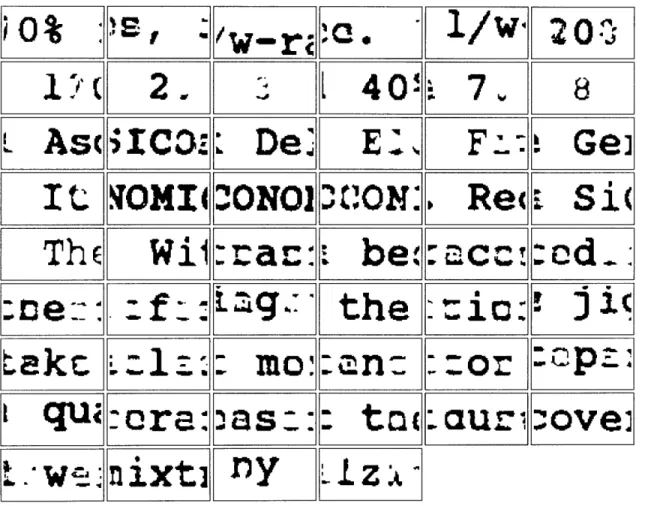
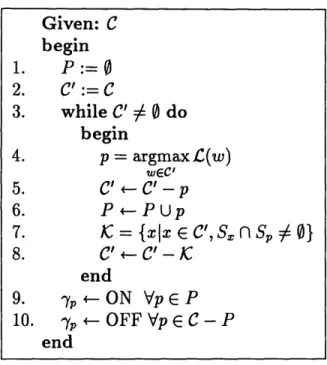
We will use the image in figure 3-3 to illustrate the procedure we have just described. The image was obtained by scanning the original image at a resolution of 300dpi. Figure 3-4 shows the locations of all the character origins on the page. The origins were obtained by running a commercial OCR program on the image that returned bounding box information on each character, as well as a label corresponding to the character at that location. The origin of each character was then taken to be at the lower left corner of the bounding box for that character. The recognition routines used connected components to isolate each character, and extract bounding box information from the isolated characters. In some cases, adjacent characters were connected in the observed image, such as the ry in Recovery in the second line, or mm in the first line after ECONOMICS, and were identified as a single character and labeled as the first observed character. For this reason, only the first glyph in these cases

has an origin, the other glyph was not given an individual label or an origin by the recognizer.

With the origins known, we proceed to obtain the observed instances of a character by extracting a fixed size image region about each of the origins of that character. Figure 3-5 shows all the observed instances of the character "a". Note the proper image for the "a" is in the middle of all the canvasses, and surrounded by complete and partial images of other characters. There are slight differences between each of the observed instances of the "a", particularly in the edges and in the thickness of each glyph. These are the variations that the ML template tries to capture through the noise mode]. In the estimation procedure we implicitly assume that the presence of other character images are extreme artifacts due to the noise model. This is not true, and in the next section we discuss how to deal with them.

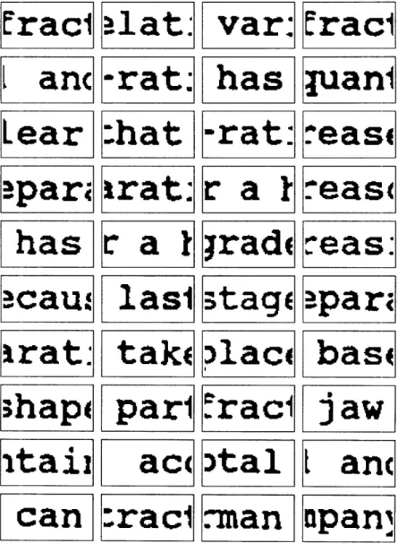
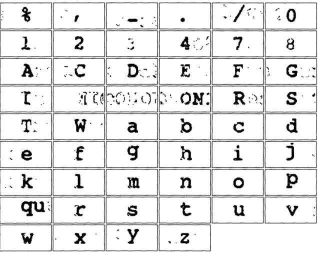
Figure 3-6 shows all the ML templates after having applied the Maximum Likeli-hood template estimation routine to all the observed images of each character. Note the presence of the proper support in each character template. In the case of the "h", notice the marked presence of the corresponding images for the characters "t" and "e" to either side. This is because the character "h" occurred most frequently in the word the, and the pattern for the "t" and the "e" cannot be distinguished from the one for the "h". There are a few degenerate cases to observe, namely the templates for the "M" and for the "N". Both these character occur only once in the original image, and the best estimate for each one is simply the observed instance.

Figure 3-7 shows the Maximum Likelihood template reconstructed image. The template reconstructed image is generated by placing the origin of each character template at all origins on the image plane that are labeled with that character, and painting the corresponding template image on the canvass. The discrepancies between the template reconstructed image and the original image are very marked. This exam-ple shows the high degree of overlap that exists between all of the imaged templates,

which is clearly in violation of the non-overlapping criterion that was emphasized by the document generation models, and results in a very unreadable reconstructed irnmage. The next section develops an approach that refines these ML templates.

83

Figure 7. Recovery of different fractions in the top of the jigbed.

The relation between the time, during which the various fractions go to the top of the bed and the 1/w-ratio has not been quantified. It is however clear that if the l/w-ratio increases, the separation of the Asg becomes more difficult or for a high recovery of SiC even impossible. For this reason the recovery has to be low for a high grade SiC product. With

increasing jig time more SiC will move to the top, because in the last

stage of the demixing process the separation will take place based on the difference in shape of the particles.

ECONOMICS

The 3-8 mm fraction of the jaw crusher product contains, according to figure 2, 20 wt percent of the total Asg/SiC mixture. With 70% SiC in

the feed and 40% recovery, 1100 ton SiC can be extracted by jigging.

According to the German mother company of Elektroschmelzwerk Delfzijl

Figure 3-3: Original Image

j4.sUP

+

N wff #SA 4 $XP .~L/Cptbp 1zi # PPP A4 3 MW .&p.1

P

H 4 g I4PP P# 4W 14P F i AgP p 34 arsac Origi lp s

.hP WPpppp _{$f> P4Pf - -j} 42p _{X 94 gw} W 4 4 _{It4W r PA + XP} -A1# pp _{A /S} -X JiP ... .... I4gf _{t 4 Aw} 44 _{PrSef bmm a I ha P.b:} 4 g4 $.S4 _j i

A J A$ p pArp At $ N

4 p p ;4. 4pi4 j4pp r$

p

.4W tan hpl ,J 44,S.ph pptL3 ;+7.p& .Xp j p

pRip .tp Me PP-my ;PPW AWNvv $; ...

Erac1

Ilanc

Lear

itaii

_can

l

c n

-rat:

:hat

Irat:

lasl

tak(

parl

ac(

:racl

var:

has

-rat:

ra~

I

Ir

a

jradE

3tagE

Dlaci

.racl

)tal

man

~racl

pani

.'eas

_I

teas

I

teas:

'-pa

_r

base

jaw

Lanc

apanl

IO

',

/W1/w20::

_

2

_-_t140:

7~

It .qOMINOO

Re Si

T.1

Re(-

_Si

ThE

_Wi:Tra

b

_c!:od:

ea

(-:ne:

:

-

:ags.:

the :io:

j3c

i qui

.

W

-

·

nixt]

ny

:

t(

. auri

:ove]

Figure 3-6: Maximum Likelihood Estimated Templates

_,"

r a:

[

Ni

aS :

]1 --l I 1-1z~ [