Quantitative performance metrics for stratospheric-resolving chemistry-climate models

(1)

HAL Id: hal-00304237

https://hal.archives-ouvertes.fr/hal-00304237

Submitted on 6 Jun 2008

HAL is a multi-disciplinary open access

archive for the deposit and dissemination of sci-entific research documents, whether they are pub-lished or not. The documents may come from teaching and research institutions in France or abroad, or from public or private research centers.

L’archive ouverte pluridisciplinaire HAL, est destinée au dépôt et à la diffusion de documents scientifiques de niveau recherche, publiés ou non, émanant des établissements d’enseignement et de recherche français ou étrangers, des laboratoires publics ou privés.

Quantitative performance metrics for

stratospheric-resolving chemistry-climate models

D. W. Waugh, V. Eyring

To cite this version:

D. W. Waugh, V. Eyring. Quantitative performance metrics for stratospheric-resolving chemistry-climate models. Atmospheric Chemistry and Physics Discussions, European Geosciences Union, 2008, 8 (3), pp.10873-10911. �hal-00304237�

(2)

ACPD

8, 10873–10911, 2008 Grading of CCMs D. W. Waugh and V. Eyring Title Page Abstract Introduction Conclusions References Tables Figures ◭ ◮ ◭ ◮ Back Close Full Screen / Esc

Printer-friendly Version Interactive Discussion Atmos. Chem. Phys. Discuss., 8, 10873–10911, 2008

www.atmos-chem-phys-discuss.net/8/10873/2008/ © Author(s) 2008. This work is distributed under the Creative Commons Attribution 3.0 License.

Atmospheric Chemistry and Physics Discussions

Quantitative performance metrics for

stratospheric-resolving chemistry-climate

models

D. W. Waugh1and V. Eyring2

1

Department of Earth and Planetary Science, Johns Hopkins University, Baltimore, MD, USA

2

Deutsches Zentrum f ür Luft- und Raumfahrt, Institut f ür Physik der Atmosph äre, Oberpfaffenhofen, Germany

Received: 11 April 2008 – Accepted: 9 May 2008 – Published: 6 June 2008 Correspondence to: D. W. Waugh (waugh@jhu.edu)

(3)

ACPD

Printer-friendly Version Interactive Discussion

Abstract

A set of performance metrics is applied to stratospheric-resolving chemistry-climate models (CCMs) to quantify their ability to reproduce key processes relevant for strato-spheric ozone. The same metrics are used to assign a quantitative measure of perfor-mance (“grade”) to each model-observations comparison shown inEyring et al.(2006).

5

A wide range of grades is obtained, both for different diagnostics applied to a single model and for the same diagnostic applied to different models, highlighting the wide range in ability of the CCMs to simulate key processes in the stratosphere. No model scores high or low on all tests, but differences in the performance of models can be seen, especially for transport processes where several models get low grades on

mul-10

tiple tests. The grades are used to assign relative weights to the CCM projections of 21st century total ozone. However, only small differences are found between weighted and unweighted multi-model mean total ozone projections. This study raises several issues with the grading and weighting of CCMs that need further examination, but it does provide a framework that will enable quantification of model improvements and

15

assignment of relative weights to the model projections.

1 Introduction

There is considerable interest in how stratospheric ozone will evolve through the 21st century, and in particular how ozone will recover as the atmospheric abundance of halogens continues to decrease. This ozone recovery is likely to be influenced by

20

changes in climate, and to correctly simulate the evolution of stratospheric ozone it is necessary to use models that include coupling between chemistry and climate pro-cesses. Many such Chemistry-Climate Models (CCMs) have been developed, and simulations using these models played an important role in the latest international as-sessment of stratospheric ozone (WMO,2007).

25

(4)

evalu-ACPD

Printer-friendly Version Interactive Discussion ation of the CCMs. A set of core validation processes relevant for stratospheric ozone,

with each process associated with one or more model diagnostics and with relevant datasets that can be used for validation, has been defined by the Chemistry-Climate Model Validation Activity (CCMVal) for WCRP’s (World Climate Research Programme) SPARC (Stratospheric Processes and their Role in Climate) project (Eyring et al.,

5

2005). Previous studies have performed observationally-based evaluation of CCMs (e.g., Austin et al., 2003; Eyring et al., 2006) using a subset of these key processes. However, although these studies compared simulated and observed fields they did not assign quantitative metrics of performance (“grades”) to these observationally-based diagnostic tests. Assigning grades to a range of diagnostics has several potential

ben-10

efits. First, it will allow easy visualization of the model’s performance for multiple as-pects of the simulations. Second, in the case of a systematic bias for all models, it will allow identification of missing or falsely modeled processes. Third, it will enable a quantitative assessment of model improvements, both for different versions of individ-ual CCMs and for different generations of community-wide collections of models used

15

in international assessments. Finally, it will make it possible to assign relative weights to the predictions by the different models and to form a best estimate plus variance that takes into account the differing abilities of models to reproduce key processes.

In this paper we perform a quantitative evaluation of the ability of CCMs to reproduce key processes for stratospheric ozone. Our starting point is the recent study byEyring 20

et al. (2006) (hereinafter “E06”) who evaluated processes important for stratospheric ozone in thirteen CCMs. We consider the same CCMs, diagnostics, and observational datasets shown in E06. This has the advantage that the model simulations, diagnos-tics, and graphical comparisons between models and observations have already been presented and don’t need to be repeated here. Also, E06 selected these diagnostics

25

as they are important for determining the ozone distribution in the stratosphere. We further simplify our approach by using the same metric to quantify model-observations differences for all diagnostics. This quantification of each CCM’s ability to reproduce key observations and processes is then used to weight ozone projections for the 21st

(5)

ACPD

Printer-friendly Version Interactive Discussion century from the same CCMs, which were analyzed inEyring et al.(2007) (hereinafter

“E07”).

Several previous studies have performed similar quantitative evaluation of atmo-spheric models, although not stratoatmo-spheric CCMs. For example, Douglass et al. (1999) and Strahan and Douglass (2004) performed a quantitative evaluation of stratospheric

5

simulations from an off-line three-dimensional chemical transport model (CTM). In these two studies they assigned grades to multiple diagnostics to assess simulations driven by different meteorological fields. Brunner et al. (2003) compared model sim-ulations of tropospheric trace gases with observations. In contrast to the comparison of climatological fields considered here, they focused on model-observations

compar-10

isons at the same time and location as the measurements. This is possible for CTMs driven by assimilated meteorological fields, but not for CCMs. More recently, several studies have performed quantitative evaluations of coupled ocean-atmosphere climate models, and formed a single performance index that combines the errors in simulat-ing the climatological mean values of many different variables (e.g.,Schmittner et al.,

15

2005;Connolley and Bracegirdle,2007;Reichler and Kim,2008). Our approach draws on several features of the above studies. Several of the diagnostics considered here were considered in Douglass et al. (1999) and Strahan and Douglass (2004), and, in a similar manner toSchmittner et al.(2005),Connolley and Bracegirdle(2007),Reichler

and Kim (2008) and Gleckler et al. (2008), we form a single performance index for

20

each model.

The methods used to evaluate the models and weight their projections are described in the next section. The models and diagnostics considered are then described in Sect. 3. Results are presented in Sect. 4, and conclusions and future work discussed in the final section.

(6)

ACPD

2 Method

2.1 General framework

The general framework used in this paper to evaluate the models and weight their predictions involves the following steps.

1. A suite of observationally-based diagnostic tests are applied to each model.

5

2. A quantitative metric of performance (grade) is assigned to the application of each observations-model comparison (diagnostic) to each model, i.e.,gjk is the grade

of thej-th diagnostic applied to the k-th model.

3. Next, the grades for each diagnostic are combined together to form a single per-formance index for each model, i.e., the single index of modelk is

10 ¯ g_k=1 W N X j=1 w_jg_jk (1) where_{W =}PN

j=1wj,N is the number of diagnostics, and wj is the weight

(impor-tance) assigned to each diagnostic. If all diagnostics have equal importance then

w_j is the same for allj .

4. Finally, the model scores are used to weight the predictions of a given quantityX

15

fromM models, i.e.

ˆ µX= 1 P ¯gk M X k=1 ¯ gkXk. (2)

(7)

ACPD

Printer-friendly Version Interactive Discussion If ¯g_k are the same for all models then this reduces to the normal multi-model

meanµX. The model scores can also be used to form a weighted variance:

ˆ σ_X2= P ¯gk (P ¯g_k)2₋_{P ¯}_g2 k M X k=1 ¯ gk(Xk− ˆµX)2. (3)

Again, if ¯gkis the same for all models then this reduces to the normal multi-model

varianceσ_X2.

5

The above framework is not fully objective as several subjective choices need to be made to apply it. For example, decisions need to be made on the diagnostics to apply, the observations to be used, the grading metric to be used, and the relative importance of the different diagnostics for predictions of quantity X . These issues are discussed below (see also discussion inConnolley and Bracegirdle,2007).

10

2.2 Grading metric

To implement the above framework a grading metric needs to be chosen. Several differ-ent metrics have been used in previous model-observation comparisons. For example, Reichler and Kim (2008) used the squared difference between model and observed climatological mean values divided by the observed variance, whereas Gleckler et

15

al. (2008) focus on the root mean squared difference between the model and observed climatological mean values. In this study we wish to use a grading metric that can be applied to all diagnostics, and can easily be interpreted and compared between tests. We choose the simple diagnostic used by Douglass et al. (1999)

g=1 −_n1

g

|µmodel− µobs|

σ_obs (4)

20

whereµ_model is the mean of a given field from the model, µ_obs is the corresponding quantity from observations,σ_obs is a measure of the uncertainty (e.g. standard devia-tion) in the observations, andng is a scaling factor. Ifg=1 the simulated field matches

(8)

ACPD

Printer-friendly Version Interactive Discussion the observations, and smallerg corresponds to a larger difference between model and

observations. If_{g<0 then the model-observations difference is greater than n}_g times

σ. In our analysis we use, as in Douglass et al. (1999), n_g=3, for which g=0 if the model mean is 3σ from the observed climatological mean value. We reset negative

values ofg to zero, so g is always non-negative. As with the metrics used by

Reich-5

ler and Kim (2008) and Gleckler et al. (2008), the metricg provides a measure of the

difference in model and observed climatological means.

There are several other possible metrics. One is the statistict used in the standard

t-test (Wilks, 1995): t= µmodel− µobs σT q 1 nmodel + 1 nobs , (5) 10 where σ_T2=(nmodel− 1)σ 2 model+ (nobs− 1)σ 2 obs (n_model+ nobs− 2) .

Unlike the metricg, or the above metrics, the t-statistic involves the variance in both

the observations and models. The t-statistic has the advantage over the metric (4)

in that there is a standard procedure to determine the statistical significance of the

15

differences between models and observations from it. However, the value of t depends on the number of elements in the data sets, and it is not as easy to comparet from

different tests that use datasets with a different number of elements as for the metric g. Also, it cannot be applied to all our diagnostics as some lack long enough data records for calculation of variance in the observations.

20

Furthermore, there is in fact a close relationship betweeng and t, and the statistical

significance of the model-observations difference can be estimated from the value of

g. To see this consider the case when the models and observations have the same

(9)

ACPD

Printer-friendly Version Interactive Discussion (5) we have

t=r n

2ng(1 − g), (6)

wheren=nmodel=nobs. Given this relationship we can determine the value of t, and hence the statistical significance of the model-observations difference, from the grade

g. For example, for ng=3 a grade g=2/3 corresponds to t=

q

n/2. For n=10 this value

5

of _{t indicates that the difference between the model and observations is significant} at greater than 98% while for n=20 the difference is significant at greater than 99%.

This means that for comparisons of climatological values based on decadal or longer datasets a value ofg<2/3 is significant at greater than 98%. The above relationship

holds only in the above special case, but as shown in Sect. 4.2 it is a good

approxima-10

tion for the more general cases considered here. Hence (6) can be used to estimatet,

and the statistical significance, fromg.

In the metric (4) the errors for different diagnostics are normalized by the uncertainty in the observations. This means that the mean grade over all models for each diagnos-tic will vary if the models are better/poorer at simulating a pardiagnos-ticular process or field.

15

Also, some quantities may be more tightly constrained by observations than others, and this can be captured (by variations inσ_obs) by the metric (4). A different approach was used by Reichler and Kim (2008) and Gleckler et al. (2008), who normalized the error by the “typical” model error for each quantity. This approach means that the average grade over all models will be roughly the same for all diagnostics (around zero).

20

In summary, we use the metric (4) in our analysis because it can be applied to all the diagnostic tests, is easy to interpret, and can easily be compared between tests. Also, as shown above the statistical significance can be estimated from it.

One limitation with any metric, and in fact any comparison between models and observations, is uncertainties in the observations (and in particular, unknown biases in

25

the observations). If the observations used are biased, then an unbiased model that reproduces the real atmosphere may get a low grade, while a model that is biased

(10)

ACPD

Printer-friendly Version Interactive Discussion may get a high grade. The potential of a bias in the observational dataset used can

be assessed for diagnostics where there are several sources of data, and we consider several such cases in Sect. 4.2 below. However, for most diagnostics considered here multiple data sets are not available.

3 Models and diagnostics

5

As discussed in the Introduction we consider the CCM simulations, diagnostics, and observations that were evaluated in E06. The thirteen models considered are listed in Table1, and further details are given in E06 and the listed reference for each model.

The simulations considered in the E06 model evaluation, and used here to form model grades, are transient simulations of the last decades of the 20th century. The

10

specifications of the simulations follow, or are similar to, the “reference simulation 1” (“REF1”) of CCMVal, and include observed natural and anthropogenic forcings based on changes in sea surface temperatures (SSTs), sea ice concentrations (SICs), surface concentrations of long-lived greenhouse gases (GHGs) and halogens, solar variability, and aerosols from major volcanic eruptions. The simulations considered in E07 are

15

projections of the 21st century (“REF2” simulation), in which the Intergovernmental Panel on Climate Change (IPCC) Special Report on Emission Scenarios (SRES) A1B GHG scenario and the WMO (2003) Ab surface halogens scenario are prescribed. SSTs and SICs in REF2 are taken from coupled atmosphere-ocean model projections using the same GHG scenario.

20

The diagnostic tests applied to the past CCM simulations are listed in Table2. Each diagnostic is based on a model-observations comparison shown in E06, and the figures in E06 showing the comparison are listed in Table 2. The exception is the middle latitude Cl_y test where the comparison is shown in E07, and also Fig.1 below. Note that E06 also compared the simulated ozone with observations. However, as ozone is

25

the quantity of interest in our analysis, we focus solely on diagnostics of processes that are important for simulating ozone.

(11)

ACPD

Printer-friendly Version Interactive Discussion Many other diagnostic tests could be used in this analysis, such as those defined in

Table 2 of Eyring et al. (2005). However, for this study we focus on a relatively small number of diagnostics that have already been applied. These diagnostics were chosen by E06 as they test processes that are key for simulating stratospheric ozone. In partic-ular, the diagnostics were selected to assess how well models reproduce (a) polar

dy-5

namics, (b) stratospheric transport, and (c) water vapor distribution. Correctly simulat-ing polar ozone depletion (and recovery) requires the dynamics of polar regions, and in particular polar temperatures, to be correctly simulated. Assessing the reality of these aspects of the CCMs is thus an important component of a model assessment. Another important aspect for simulating ozone is realistic stratospheric transport. Of particular

10

importance is simulating the integrated transport time scales (e.g. mean age), which plays a key role in determining the distributions of Cl_y and inorganic bromine (Br_y). Changes in water vapor can have an impact on ozone through radiative changes, changes in HO_x, or changes in formation of polar stratospheric clouds (PSCs), and it is therefore also important to assess how well models simulate the water vapor

dis-15

tribution.

Although the model-observations comparisons have already been presented further decisions still need to be made to quantify these comparisons. For example, choices need to be made on the region and season to be used in the grading metric (4). This choice will depend on the process to be examined as well as the availability of

obser-20

vations.

Another important issue in the calculation of the grade is the assignment of σ_obs. For some quantities there are multi-year observations and an interannual standard deviation can be calculated, and in these cases we use this in metric (4). For other quantities these observations do not exist and an estimate of the uncertainty in the

25

quantity is used asσobs. This is not very satisfying, and it would be much better if in all casesσ_obs included both measurement uncertainty and variability. Note, however, that σ_obs does not impact the ranking of models for a particular test, it only impacts comparisons of the grades for different tests.

(12)

ACPD

Printer-friendly Version Interactive Discussion The regions, seasons, and observations used for each diagnostic are listed in Table2

and are described in more detail below.

– For the polar temperature diagnostic we focus on the lower stratosphere during winter and spring, as these temperatures are particularly important for modeling polar ozone depletion. Specifically we consider polar average (60–90◦N or S)

5

temperatures averaged over 50 to 30 hPa and Decmber to February (60–90◦N) or September to November (for 60–90◦S). These tests will be referred to as “Temp-NP” and “Temp-SP”, respectively. Climatological mean and interannual standard deviation of ERA-40 reanalyses (Uppala et al., 2005) for 1980-1999 are used for the observations in metric (4), and the same period is used to calculate the model

10

climatology. The biases of the models relative to ERA-40 reanalyses are shown in Fig. 1 of E06.

– The transition to easterlies diagnostic (“U-SP”) measures the timing of the break down of the Antarctic polar vortices in the CCMs. It is based on Fig. 2 of E06, which shows the timing of the transition from westerlies to easterlies for

zonal-15

mean zonal winds at 60◦S. The grade is determined using the date for the transi-tion at 20 hPa, and climatological ERA-40 reanalysis for the observatransi-tions.

– The vertical propagation of planetary waves into the stratosphere plays a signif-icant role in determining polar temperatures during winter and spring (Newman et al., 2001). This wave forcing can be diagnosed with the mid-latitude 100 hPa

20

eddy heat flux for the regions and periods shown in Fig. 3 of E06: 40◦–80◦N for January-February (“HFlux-NH”), or 40◦–80◦S for July–August (“HFlux-SH”). This is only one aspect of the information shown in this figure, and grades could also be based, for example, on the slope of the heat flux – temperature relationship.

– The tropical tropopause temperature diagnostic (“Temp-Trop”) is based on the

25

tropical temperature at 100 hPa, shown in Fig. 7a of E06. For this diagnostic Eq. (4) is applied for each month separately, using ERA-40 climatological mean

(13)

ACPD

Printer-friendly Version Interactive Discussion and interannual standard deviation for the observations, and then the average of

these 12 values is used as the single grade for this diagnostic.

– The entry water vapor diagnostic (“H₂O-Trop”) is based on the tropical water va-por at 100 hPa, see Fig. 7b of E06. As for the tropical tropopause temperature diagnostic Eq. (4) is applied for each month separately, this time using HALOE

cli-5

matological mean and interannual standard deviation for the observations (Grooß and Russell, 2005), and the average of these 12 values is used as the single grade. The model climatology is for 1990–1999, whereas the HALOE observa-tions are for 1991–2002.

– The three tracer gradient diagnostics are based on comparisons of the

simu-10

lated and observed methane (CH₄) distributions, see Fig. 5 of E06. We focus on lower stratospheric gradients, and use these diagnostics to assess the lower stratospheric transport in the tropics and polar regions. As CH₄ at the tropical tropopause (100 hPa) is very similar in all models and observations we use the tropical (10◦S–10◦N) averaged values between 30 and 50 hPa to quantify

differ-15

ences in vertical tracer gradients in the tropical lower stratosphere (“CH₄-EQ”). Similarly, we use October CH₄at 80◦S averaged values between 30 and 50 hPa to quantify differences in vertical tracer gradients in the Antarctic lower strato-sphere (“CH₄-SP”). We do not include a similar diagnostic at 80◦N as HALOE rarely samples 80◦N, even if equivalent latitude is used. For subtropical

merid-20

ional gradients we use the difference in 50 hPa CH4between 0◦N and 30◦N, for March and between 0◦N and 30◦S for October (“CH₄-Subt”). A grade is deter-mined for each month separately, and then averaged together to form a single grade for subtropical gradients.

– Diagnostics of the water vapor tape recorder (Mote et al., 1996) test the ability of

25

models to reproduce the amplitude and phase propagation of the annual cycle in tropical water vapor, which in turn tests the model’s tropical transport. As in Hall et al. (1999), we use the phase speedc (“Tape-c”) and attenuation of the

(14)

ampli-ACPD

Printer-friendly Version Interactive Discussion tudeR (“Tape-R”) to quantify the ability of the models to reproduce the observed

propagation of the H₂O annual cycle. The attenuation_{R=H/λ, where λ=c×1yr} is the vertical wavelength andH is the attenuation scale height of the amplitude, A= exp(−z/H). The values of c (R) are determined from linear (exponential) fits to

the simulated phase lag (relative amplitude) from the level of maximum amplitude

5

to 10 km above this level, and compared with similar calculations using HALOE observations (see Fig. 9 of E06).

– The mean age diagnostics are based on comparisons of the simulated with ob-served mean age at 50 hPa and 10 hPa shown in Fig. 10 of E06. The mean age is an integrated measure of the transport in the stratosphere, and together with tape

10

recorder diagnostics place a stringent test on models transport (e.g. Waugh and Hall, 2002). At each pressure level Eq. (4) is applied separately for the tropics (10◦S–10◦N) and northern mid-latitudes (35◦N–55◦N), and then the average of these 2 values is used as the single grade for each pressure level (“Age-10hPa” and “Age-50hPa”). Balloon observations are used for mean values and

uncer-15

tainity at 10 hPa (see symbols in Fig. 10b of E06), whereas ER2 observations are used for 50 hPa (Fig. 10c of E06).

– The Cl_y diagnostics are based on comparisons with the observed lower strato-spheric (50 hPa) Cl_y shown in Fig. 12 of E06 and Fig. 1 of E07, and repeated in Fig.1. We calculate grades separately for spring in the southern polar region

20

(80◦S, October; “Cly-SP”) and for annual-mean values in northern mid-latitudes (30◦–60◦N; “Cly-Mid”). The observed mean values and uncertainties used are the same as shown in Fig.1. As the REF1 simulation in some models stops at the end of 1999, only observations in the 1990s are used in calculating the grade.

(15)

ACPD

4 Results

4.1 Model grades

The diagnostic tests listed in Table 2 have been applied to the thirteen CCMs listed in Table 1 and gradesg determined using metric (4). We also calculate the grade for the

“mean model”, i.e., the mean over all models is calculated for the various quantities

5

listed in Table 2, and then a grade is calculated using this mean value in the metric (4). We consider first, as an example, the grades of the Cl_y tests. Figure 1 shows the time series of mid-latitude and polar Cl_y at 50 hPa from the 13 models, together with observations and the mean of the models. As discussed in E06 there is a large spread in the modeled Cl_y, and some large model-observations differences. For polar Cly,

10

models 1, 11, and 12 produce values close to the observations, and these models have grades around 0.9 forn_g=3 (see second to bottom row in Fig.2). However, most of the models produce polar Cl_y much lower than observed, and several models are more than 3σ from the mean observations and have a grade of 0 (as noted above,

values ofg less than zero are reset to zero). Models 4 and 9 are in fact more than 5σ

15

from the mean observations. For mid-latitude Cl_y the model-observations differences are not as large as for polar Cl_y. Several models are withinσ of the mean value (and

haveg>0.66) and only one model (model 4) is 3 σ away from the mean value. Note

the model 8 has a high grade for mid-latitude Cl_y because it agrees with observations before 2000, but Fig. 1 shows that the Cl_y in this model continues to increase and

20

deviates from observations after 2000. If these later measurements were used the grade for this model would be much lower.

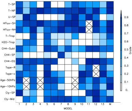
We now consider the grades for all diagnostics. The results of the application of each test to each model are shown in Fig. 2. In this matrix (“portrait” diagram) the shading of each element indicates the grade for application of a particular diagnostic

25

to a particular model (a cross indicates that this test could not be applied, because the required output was not available from that model). Each row corresponds to a different diagnostic test (e.g. bottom two rows showg for the two Cly tests), and each column

(16)

ACPD

Printer-friendly Version Interactive Discussion corresponds to a different model. The grades for the “mean model” are shown in the

right-most column.

Figure 2 shows that there is a wide range of grades, with many cases with g≈0

and also many cases withg>0.8. These large variations in g can occur for different

diagnostics applied to the same model (e.g., most columns in Fig.2) or for the same

5

diagnostic applied to different models (e.g., most rows in Fig. 2). The wide range in the ability of models to reproduce observations, with variations between models and between different diagnostics, can be seen in the figures in E06. This analysis quantifies these differences and enables presentation in a single figure.

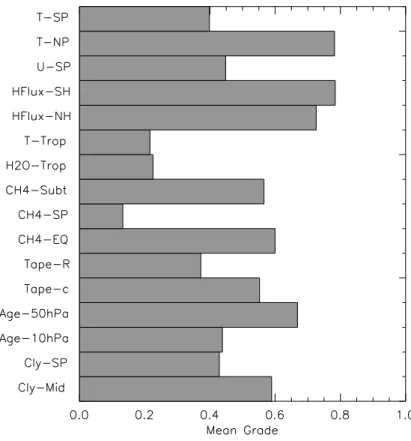
The wide range of grades for all diagnostic tests shows that there are no tests where

10

all models perform well or all models perform poorly. However, the majority of models perform well in simulating north polar temperatures and NH and SH heat fluxes (mean grades over all models are larger than 0.7), and, to a lesser degree, mid-latitude age (mean grade greater than 0.6), see Fig.3. At the other extreme the majority of models perform poorly for the Tropical Tropopause Temperature, Entry Water Vapor, and Polar

15

CH₄tests (mean grades less than or around 0.2). Note that caution should be applied when comparing grades from different diagnostics as g is sensitive to the choice of σ, e.g., use of a smaller σ in a test results in lower grades, and some of the variations

between diagnostics could be due to differences in the assigned σ.

Figure 2 also shows that there are no models that score high on all tests or score

20

low on all tests. However, differences in the performance of models can be seen and quantified. For example, several models get low grades on multiple tests, i.e., models 4, 7, 8, and 9 haveg near zero for 4 or more transport tests. The poorer performance

of these models for several of the transport diagnostics was highlighted in E06.

To further examine the difference in model performance we compare a single

perfor-25

mance index calculated from the average grades ( ¯gk) for each model. This is shown

in Fig.4a, where the average grade is calculated assuming that all diagnostic tests are equally important (i.e., w_j=1 in Eq. 1). If a grade is missing for a particular test and model (crosses in Fig.2) then this test is not included in the average for that model.

(17)

ACPD

Printer-friendly Version Interactive Discussion There is a large range in the average performance of the models, with ¯g varying from

around 0.2 to around 0.7. The value of ¯g changes with ng but there is a very similar

variation between models and the ranking of models for different ng. For example,

usingn_g=5 results in a grade around 0.1 larger, for all diagnostics.

The average grade for a model can also be calculated separately for diagnostics

5

that are determined by transport or polar dynamics diagnostics, see Fig. 4b and c. The tropical tropopause temperature and H₂O diagnostics are not included in either the polar dynamics or transport averages. The range of model performance for the transport diagnostics is larger than the performance for dynamics diagnostics, with ¯g

varying from around 0.1 to around 0.8. Figure4also shows that some models simulate

10

the polar dynamics much better than the transport (e.g., models 4, 8, and 9) while the reverse is true for others (e.g., models 6 and 13). Part of this could be because the dynamics tests focus on polar dynamics, whereas the majority of the transport diagnostics measure, or are dependent, on tropical lower stratospheric transport.

It is of interest to compare the model average grades shown in Fig.4with the

seg-15

regation of models made by E07. In the plots in E06 and E07 solid curves were used for fields from around half the CCMs and dashed curves for the other CCMs, and E07 stated that CCMs shown with solid curves are those that are in general in good agreement with the observations in the diagnostics considered byEyring et al.(2006). In making this separation E06 put more emphasis on the transport diagnostics than

20

the temperature diagnostics, with most weight on Cl_y comparisons. As a result the separation used in the E06 and E07 papers is not visible in the mean grades over all diagnostics but can be seen in the average of the transport grades is considered. The models shown as solid curves in E06 and E07 (models 2, 3, 5, 6, 12, and 13) all have high average transport grades, while nearly all those shown with dashed curves

25

have low average transport grades. The exceptions are models 1 and 11 which were shown as dashed curves in E06 and E07 but whose average transport grades in Fig.4

are high. The reasons for this difference is, as mentioned above, that E06 put high weight on the comparisons with Cl_y. Models 1 and 11 significantly overestimate the

(18)

ACPD

Printer-friendly Version Interactive Discussion mid-latitude Cl_yand have a very low score for the mid-latitude Cl_ytest (Fig.2).

Another interesting comparison is between the grades of individual models and that of the “mean model”. Analysis of coupled atmosphere-ocean climate models has shown that the “mean model” generally scores better than all other models (e.g. Gleck-ler et al., 2008). This is not however the case for the CCMs examined here (see right

5

most column of Fig. 2). For some of the diagnostics the grade of the mean model is larger than or around the grade of the best individual model, e.g., the NH polar temperatures, heat flux, 10 hPa mean age, and mid-latitude Cl_y diagnostics (see right most column in Fig.2). However, for most diagnostics the grade for the mean model is smaller than that of some of the individual models, with a large difference for the

10

transition to easterlies, south polar CH₄, tape recorder attenuation, and polar Cl_y di-agnostics. In these latter diagnostics there is significant bias in most, but not all, of the models, and this bias dominates the calculation of the mean of the models and the grade of the mean model is less than 0.3. But for each of these diagnostics there is at least one model that performs well (e.g.,g around or greater than 0.8), and has

15

a higher grade than the mean model. The contrast between a diagnostic where the grade for the mean model is higher than or around the best individual models and a diagnostic where the grade for the mean model is lower than many individual models can be seen in Fig.1. In panel (a) the Cl_yfor individual models is both above and below the observations, and the mean of the models is very close to the observations (and

20

has a high grade). In contrast, in panel (b) most models underestimate the observed Cl_yand the mean Cl_y is much lower than the observations (and several models). 4.2 Sensitivity analysis

As discussed above several choices need to be made in this analysis. A detailed ex-amination of the sensitivity to these choices is beyond the scope of this study. However,

25

a limited sensitivity analysis has been performed for some tests.

We first consider the sensitivity of the grades to the source of the observations. We focus on diagnostics based on the temperature field, as data are available from

(19)

dif-ACPD

Printer-friendly Version Interactive Discussion ferent meteorological centers. Figure 5 shows the grades for the (a) Temp-NP, (b)

Temp-SP, and (c) Temp-Trop tests when different meterological analyses are used for the observations. The grades for Temp-NP (panel a) are not sensitive to whether the ERA40, NCEP stratospheric analyses (Gelman et al., 1996) or UK Met Office (UKMO) assimilated stratospheric analyses (Swinbank and ONeill, 1994) are used as the

obser-5

vations. This is because the climatological values from the three analyses are very sim-ilar (within 0.2 K), and the differences between analyses is much smaller than model-observations differences (see Fig. 1 of E06). There is larger sensitivity for Temp-SP (panel b) as there are larger differences between the analyses. However, the general ranking of the models is similar which ever meteorological analyses are used in the

10

grading, i.e., models 1, 5 and 9 have high grades and models 4, 6 and 7 have low grades for all 3 analyses.

The above insensitivity to data source does not, however, hold for the Temp-Trop diagnostic. Here there are significant differences between the meteorological analyses, and the model grades vary depending on which data source is used. The climatological

15

mean UKMO values are around 1 to 2 K warmer than those of ERA40, depending on the month (see Fig. 7 of E06), and as a result very different grades are calculated for some models, see Fig.5c. For models that are colder than ERA40 lower grades are calculated if UKMO temperatures are used in the metric (e.g., models 3, 5, 9, 12, and 13), whereas the reverse is true for models that are warmer than ERA40 (models 4, 6,

20

7, 8 and 10).

The above sensitivity to meteorological analyses highlights the dependence of the grading, and any model-data comparison, on the accuracy of the observations used. It is therefore important to use the most accurate observations in the model-data com-parisons. With regard to the temperature datasets used above, intercomparisons and

25

comparisons with other datasets have shown that some biases exist in these meteo-rological analyses. In particular, the UKMO analyses have a 1–2 K warm bias at the tropical tropopause, and the NCEP analyses have a 2–3 K warm bias at the tropical tropopause and a 1–3 K warm bias in Antarctic lower stratosphere during winter-spring

(20)

ACPD

Printer-friendly Version Interactive Discussion (Randel et al., 2004). Given these biases, it is more appropriate to use, as we have,

the ERA40 analyses for the model grading.

Another choice made in the analysis is the metric used to form the grades. As discussed in Sect. 2.2, an alternate metric to the one used here is thet-statistic. It was

shown in Sect. 2.2 that there is a simple linear relationship betweent and g in cases

5

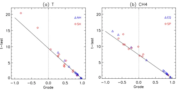
with the same number of data points and same standard deviations for the models and observations (see Eq. 6). To test this in a more general case we comparet and g for tests using temperature and CH₄ fields. For these tests there are multi-year observational data sets, and the mean and variance from these observations and from the models can be used to calculatet and g.

10

Figure6shows this comparison for the (a) Temp-NP and Temp-SP, and (b) CH₄-EQ and CH₄-SP diagnostic tests. For these comparisons we do not set negative values of

g to zero, so that we can test how well the relationship (6) holds. (If we set negative g to zero then the points left of the vertical dashed lines move to the left to lie on this

line.) As expected there is a very close relationship between the calculated values

15

oft and g, and an almost identical ranking of the models is obtained for both metrics.

Furthermore, the values oft are close to those predicted by (6), which are shown as the

solid lines in Fig.6. The deviations from this linear relationship are due to differences inσ between models and observations. The above shows that a very similar ranking

of the models will be obtained whethert or g are used, and the results presented here

20

are not sensitive to our choice ofg as the metric.

4.3 Relationships among diagnostics

We now examine what, if any, correlations there are between grades for different diag-nostics. If a strong correlation is found this could indicate that there is some redundancy in the suite of diagnostics considered, i.e., two or more diagnostics could be testing the

25

same aspects of the models. Identifying and removing these duplications from the suite of diagnostics would make the model evaluation more concise. However, an alternative explanation for a connection between grades for different diagnostics could be that the

(21)

ACPD

Printer-friendly Version Interactive Discussion models that perform poorly for one process also perform poorly for another process. In

this case the two diagnostics are not duplications, and the consideration of both might provide insights into the cause of poor performance.

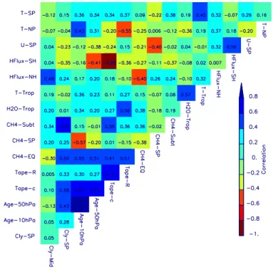
Figure7shows the correlation between the grades for each of the different diagnos-tics. There are generally low correlations between the grades, which indicates that in

5

most cases the tests are measuring different aspects of the model performance. There are however some exceptions, and several notable features in this correlation matrix.

As might be expected, several of these high correlations occur between grades for diagnostics based on the same field, e.g. between the two mean age diagnostics and the two tape recorder diagnostics. There might, therefore, be some redundancy in

10

including two grades for each of these quantities, e.g., it might be possible to consider a single grade for mean age which considers just a single region or averages over all regions. However, this is not the case for all fields, and there are low correlations between the two Cl_ydiagnostics, between the two polar temperature diagnostics, and between the CH₄ diagnostics. Thus diagnostics using the same fields can measure

15

different aspects of the simulations, and averaging into a single grade might result in loss of information.

High correlations between grades might also be expected for some pairs of diagnos-tics that are based on different fields but are dependent on the same processes. One example are the Temp-Trop and H₂O-Trop diagnostics. As the water vapor entering the

20

stratosphere is dependent on the tropical tropopause temperature a high correlation is expected between these two diagnostics. There is indeed a positive correlation, but the value of 0.48 may not be as high as expected. The fact that the correlation is not higher is mainly because of two models, whose performance differs greatly for these two diagnostics. The 100 hPa temperature in model 2 is much colder than observed

25

(with a zero grade for this diagnostic) but the 100 hPa water vapor is just outside 1σ

of the observed value (_{g=0.61). The reverse is true for model 9, which has a low} wa-ter vapor grade but reasonable temperature grade. For the remaining models, models with low grades for the tropical temperature tend to have low grades for the water vapor

(22)

ACPD

Printer-friendly Version Interactive Discussion diagnostic, and there is a much higher correlation (0.88). A higher correlation is found

between the tropical cold point and 100 hPa water vapor correlation (Gettelman et al., 2008), but the above two models are still anomalous. The sensitivity of the correla-tions to results of two models illustrates that care should be taken interpreting these correlations. It also suggests problems with, and need for further analysis of, the two

5

anomalous models that do not display the physically expected relationship between tropical tropopause temperature and entry water vapor.

There are high positive correlations between many of the transport diagnostics, i.e., there are generally high correlations between the tape recorder, mean age, and equa-torial CH₄diagnostics. This is likely because these diagnostics measure, or are

depen-10

dent, on tropical lower stratospheric transport, and a model with good (poor) transport in the tropical lower stratosphere will have good (poor) grades for all these diagnostics. Another area where strong correlations might be expected is between the heat flux, polar temperatures, and transition to easterlies diagnostics. However, in general, the correlations between these fields is not high. The exception is the high correlation

15

(0.75) between the eddy heat flux and transition to easterlies in the southern hemi-sphere. A high correlation between these diagnostics might be expected as weak heat fluxes might lead to a late transition. However, this is not likely the cause of the high correlation. First, the heat flux diagnostic is for mid-winter (July–August) and the late-winter/spring heat fluxes are likely more important for the transition to easterlies. More

20

importantly, several of the models with late transitions, and very low grades for this diagnostic, actually have larger than observed heat fluxes (models 1, 5 and 13), which is opposite than expected from the above arguments. Again, this anomalous behavior suggests possible problems with these models and the need for further analysis.

Figure7also shows some correlation between the transport and dynamics

diagnos-25

tics. In fact there are several cases where there is moderate to high negative correla-tions between a dynamics diagnostic and a transport diagnostic, suggesting that there are models that perform poorly for (tropical) transport diagnostics but perform well for (polar) dynamical diagnostics. As discussed above this is indeed the case for several

(23)

ACPD

Printer-friendly Version Interactive Discussion models (most notably models 8 and 9) see Fig.4).

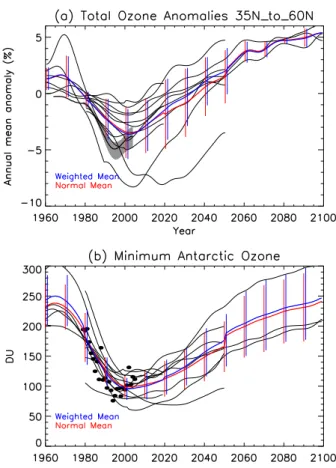
4.4 Weighted ozone projections

The assignment of grades to the diagnostic tests enables relative weights to be as-signed to the ozone projections from different models, and for a weighted mean to be formed that takes into account differing abilities of models to reproduce key processes.

5

We explore this issue using ozone projections for the 21st century made by the same CCMs, and shown in E07. Note, models 6 and 11 did not perform simulations into the future, and the analysis below is only for the other 11 models listed in Table 1.

E07 examined the model projections of total column ozone for several different re-gions and for different diagnostics of polar ozone. We focus here on two ozone

diagnos-10

tics: (a) annual mean northern mid-latitude total ozone (Fig. 5 of E07) and (b) minimum Antarctic total column ozone for September to October (Fig. 8b of E07). Similar results are found for all total ozone quantities shown in E07.

To form a weighted mean it is necessary to form a single performance index for each model (e.g. ¯gk in Eq. 1). If all diagnostics considered here are given equal weight then

15

the weighted mean using these indices is very similar to the unweighted mean (not shown). If however, the performance index is based only on the transport diagnostics there is a larger variation between models (see Fig.4), and some differences between weighted and unweighted may be expected.

To examine these differences we compare the unweighted and weighted mean using

20

model indices based on the average transport grade. We are using this index for the weighting only for illustrative purposes, and not to imply this is the best index to use. In Fig. 8 the ozone for individual models is shown as black curves, the unweighted mean in red, and the weighted mean in blue. The jumps in the mean curves, e.g. at 2050, occur because not all model simulations cover the whole time period, and there

25

is a change in the number of model simulations at the location of the jumps, e.g. eight models performed simulations to 2050, but only three models simulate past 2050.

(24)

ACPD

Printer-friendly Version Interactive Discussion only small differences between the weighted and unweighted mean values, even when

only transport diagnostics are used for the weighting. This is because there is a wide range in the ozone projections, and for most time periods models that simulate ozone at opposite extremes have similar grades. For example, there are large differences (≈100 DU) in minimum Antarctic ozone after 2050 between one of the three models

5

and the other two, but the three models have similar average grades ( ¯g≈0.6–0.7) and

the unweighted and weighted means are very similar. The largest difference between unweighted and weighted means occurs between 2030 and 2050. This difference is primarily because of the ozone and index for model 8. During this period model 8 predicts much lower ozone than the other models (the black curve with lowest ozone

10

between 2020 and 2050 is model 8), but this model has a low index (≈0.2) which means that less weight is put on the ozone from this model in the weighted mean. As a result the weighted mean is larger than the unweighted mean.

The conclusion from the above analysis is that, at least for these CCM simulations, weighting the model results does not significantly influence the multimodel mean

pro-15

jection of total ozone. A similar conclusion was reached by Stevenson et al. (2006) in their analysis of model simulations of tropospheric ozone, and bySchmittner et al.

(2005) in their analysis of the thermohaline circulation in coupled atmosphere-ocean models.

5 Conclusions

20

The aim of this study was to perform a quantitative evaluation of stratospheric-resolving chemistry-climate models (CCMs). To this end, we assigned a quantitative metric of performance (grade) to each of the observationally-based diagnostics applied inEyring

et al. (2006). The same metric was applied to each diagnostic, and the ability of the thir-teen CCMs to simulate a range of processes important for stratospheric ozone

quanti-25

fied.

(25)

ACPD

Printer-friendly Version Interactive Discussion of grades were obtained, showing that there is a large variation in the ability of the

CCMs to simulate different key processes. This large variation in grades occurs both for different diagnostics applied to a single model and for the same diagnostic applied to different models. No model scores high or low on all tests, but differences in the performance of models can be seen. This is especially true for transport processes

5

where several models get low grades on multiple transport tests, as noted in Eyring

et al. (2006).

The assignment of grades to diagnostic tests enables a single performance index to be determined for each CCM, and for relative weights to be assigned to model projec-tions. Such a procedure was applied to the CCMs’ projections of 21st century ozone

10

(Eyring et al.,2007). However, only small differences are found between weighted and unweighted multi-model mean ozone projections, and weighting these model projec-tions based on the diagnostic tests applied here does not significantly influence the results.

Although the calculation of the grades and weighting of the ozone projections is

rel-15

atively easy, there are many subjective decisions that need to be made in this process. For example, decisions need to be made on the grading metric to be used, the source and measure of uncertainty of the observations, the set of diagnostics to be used, and the relative importance of different processes/diagnostics. We have performed some limited analysis of the sensitivity to these choices, and Gleckler et al. (2008) have

dis-20

cussed these issues in the context of atmosphere-ocean climate models. However, further studies are required to address this in more detail. In particular, determining the relative importance of each diagnostic is not straightforward, and more research is needed to determine the key diagnostics and the relative importance of each of these diagnostics in the weighting.

25

This study provides only an initial step towards a quantitative grading and weighting of CCM projections. We have evaluated only a subset of key processes important for stratospheric ozone, in particular we have focused on diagnostics to evaluate transport and dynamics in the CCMs and to a lesser extent the representation of chemistry

(26)

ACPD

Printer-friendly Version Interactive Discussion and radiation. Also we have only evaluated the climatological mean state and not

the ability of the models to represent trends and interannual variability. However, this study does provide a framework, and benchmarks, for the evaluation of new CCMs simulations, such as those being performed for the upcoming SPARC CCMVal Report (http://www.pa.op.dlr.de/CCMVal/).

5

Acknowledgements. We acknowledge the CCM groups of AMTRAC (GFDL, USA), CCSRNIES (NIES, Tsukuba, Japan), CMAM (MSC, University of Toronto and York University, Canada), E39C (DLR Oberpfaffenhofen, Germany), GEOSCCM (NASA/GSFC, USA), LMDZrepro (IPSL, France), MAECHAM4CHEM (MPI Mainz, Hamburg, Germany), MRI (MRI, Tsukuba, Japan), SOCOL (PMOB/WRC and ETHZ, Switzerland), ULAQ (University of LAquila, Italy), UMETRAC

10

(UK Met Office, UK, NIWA, NZ), UMSLIMCAT (University of Leeds, UK), and WACCM (NCAR, USA) for providing their model data for the CCMVal Archive. Co-ordination of this study was supported by the Chemistry-Climate Model Validation Activity (CCMVal) for WCRP’s (World Climate Research Programme) SPARC (Stratospheric Processes and their Role in Climate) project. We thank the British Atmospheric Data Center for assistance with the CCMVal Archive.

15

This work was supported by grants from NASA and NSF.

References

Akiyoshi, H., Sugita, T., Kanzawa, H., and Kawamoto, N.: Ozone perturbations in the Arc-tic summer lower stratosphere as a reflection of NOx chemistry and planetary scale wave

activity, J. Geophys. Res., 109, D03304, doi:10.1029/2003JD003632, 2004.

20

Austin, J.: A three-dimensional coupled chemistry-climate model simulation of past strato-spheric trends, J. Atmos. Sci., 59, 218–232, 2002.

Austin, J., Shindell, D., Beagley, S. R., Bruhl, C., Dameris, M., Manzini, E., Nagashima, T., Newman, P., Pawson, S., Pitari, G., Rozanov, E., Schnadt, C., and Shepherd, T. G.: Uncer-tainties and assessments of chemistry-climate models of the stratosphere, Atmos. Chem.

25

Phys., 3, 1–27, 2003,

http://www.atmos-chem-phys.net/3/1/2003/.

(27)

ACPD

stratospheric age of air in coupled chemistry-climate model simulations, J. Atmos. Sci., 64, 905–921, 2006.

Brunner, D., Staehlin, J., Rogers, H. L., et al.: An evaluation of the performace of chemistry transport models by comparison with research aircraft observations – Part 1: Concepts and overall model performance, Atmos. Chem. Phys., 3, 1609–1631, 2003

5

Connolley, W. M. and Bracegirdle, T. J.: An Antarctic assessment of IPCC AR4 climate models, Geophys. Res. Lett., 34, L22505, doi:10.1029/2007GL031648, 2007.10876,10878

Dameris, M., Grewe, V., Ponater, M., Deckert, R., Eyring, V., Mager, F., Matthes, S., Schnadt, C., Stenke, A., Steil, B., Br ¨uhl, C., and Giorgetta, M.: Long-term changes and variability in a transient simulation with a chemistry-climate model employing realistic forcings, Atmos.

10

Chem. Phys., 5, 2121–2145, 2005,

Douglass, A. R., Prather, M. J., Hall, T. M., Strahan, S. E., Rasch, P. J., Sparling, L. C., Coy, L., and Rodriguez, J. M.: Choosing meteorological input for the global modeling initiative assessment of high-speed aircraft, J. Geophys. Res., 104, 27 545–27 564, 1999.

15

Egorova, T., Rozanov, E., Zubov, V., Manzini, E., Schmutz, W., and Peter, T.: Chemistry-climate model SOCOL: a validation of the present-day climatology, Atmos. Chem. Phys., 5, 1557– 1576, 2005,

Eyring, V., Harris, N. R. P., Rex, M., et al.: A strategy for process-oriented validation of coupled

20

chemistry-climate models, Bull. Am. Meteorol. Soc., 86, 1117–1133, 2005.

Eyring, V., Butchart, N., Waugh, D. W., et al.: Assessment of temperature, trace species, and ozone in chemistry-climate model simulations of the recent past, J. Geophys. Res., 111, D22308, doi:10.1029/2006JD007327, 2006. 10874,10875,10888,10895,10896

Eyring, V., Waugh, D. W., Bodeker, G. E., et al.: Multimodel projections of stratospheric ozone in

25

the 21st century, J. Geophys. Res., 112, D16303, doi:10.1029/2006JD008332, 2007.10876,

10896

Fomichev, V. I., Jonsson, A. I., de Grandpr ´e, J., Beagley, S. R., McLandress, C., Semeniuk, K., and Shepherd, T. G.: Response of the middle atmosphere to CO2 doubling: Results from

the Canadian Middle Atmosphere Model, J. Climate, 20, 1121–1144, 2007.

30

Garcia, R. R., Marsh, D., Kinnison, D., Boville, B., and Sassi, F.: Simulations of sec-ular trends in the middle atmosphere, 1950-2003, J. Geophys. Res., 112, D09301, doi:10.1029/2006JD007485, 2007.

(28)

ACPD

Gelman, M. E., Miller, A. J., Johnson, K. W., and Nagatani, R.: Detection of long-term trends in global stratospheric temperature from NMC analyses derived from NOAA satellite data, Adv. Space Res., 6, 17–26, 1996.

Gettelman, A., Birner, T., Eyring, V., Akiyoshi, H., Plummer, D. A., Dameris, M., Bekki, S., Lefevre, F., Lott, F., Br ¨uhl, C., Shibata, K., Rozanov, E., Mancini, E., Pitari, G., Struthers,

5

H., Tian, W., and Kinnison, D. E.: The Tropical Tropopause Layer 1960-2100, Atmos. Chem. Phys. Discuss., 8, 1367–1413, 2008,

http://www.atmos-chem-phys-discuss.net/8/1367/2008/.

Gleckler, P.J, Taylor, K. E., and Doutriaux, C.: Performance Metrics for Climate Models, J. Geophys. Res., 113, D06104, doi: 10.1029/2007JD008972, 2008.10876

10

Grooß, J.-U. and Russell III, J. M.: Technical note: A stratospheric climatology for O3, H2O,

CH4, NOx, HCl and HF derived from HALOE measurements, Atmos. Chem. Phys., 5, 2797–

2807, 2005,

Hall, T. M., Waugh, D. W., Boering, K. A., and Plumb, R. A.: Evaluation of transport in

strato-15

spheric models, J. Geophys. Res., 104, 18 815–18 840, 1999.

Lott, F., Fairhead, L., Hourdin, F., and Levan P.: The stratospheric version of LMDz: Dynamical Climatologies, Arctic Oscillation, and Impact on the Surface Climate, Climate Dynamics, 25, 851–868, doi:10.1007/s00382-005-0064, 2005.

Mote, P. W., Rosenlof, K. H., McIntyre, M. E., Carr, E. S., Gille, J. C., Holton, J. R., Kinnersley,

20

J. S., Pumphrey, H. C., Russell III, J. M., and Waters, J. W.: An atmospheric tape recorder: The imprint of tropical tropopause temperatures on stratospheric water vapor, J. Geophys. Res., 101, 3989–4006, doi:10.1029/95JD03422, 1996.

Newman, P. A., Nash, E. R., and Rosenfield J. E.: What controls the temperature of the Arctic stratosphere during spring?, J. Geophys. Res., 106, 19 999–20 010, 2001.

25

Pawson, S., Stolarski, R. S., Douglass, A. R., Newman, P. A., Nielsen, J. E., Frith, S. M., and Gupta, M. L.: Goddard Earth Observing System Chemistry-Climate Model Simulations of Stratospheric Ozone-Temperature Coupling Between 1950 and 2005, J. Geophys. Res, in press, 2008.

Pitari, G., Mancini, E., Rizi, V., and Shindell, D.: Feedback of future climate and sulfur emission

30

changes an stratospheric aerosols and ozone, J. Atmos. Sci., 59, 414–440, 2002.

Randel, W., Udelhofen, P., Fleming, E., et al.: The SPARC Intercomparison of Middle-Atmosphere Climatologies. J. Climate, 17, 986–1003, 2004.

(29)

ACPD

Reichler, T. and Kim, J.: How well do coupled models simulate today’s climate?, Bull. Am. Meteor. Soc., 89, 303–311, doi:10.1175/BAMS-89-3-303, 2008.10876

Shibata, K. and Deushi, M.: Partitioning between resolved wave forcing and unresolved gravity wave forcing to the quasi-biennial oscillation as revealed with a coupled chemistry-climate model, Geophys. Res. Lett., 32, L12820, doi:10.1029/2005GL022885, 2005.

5

Schmittner, A., Latif, M., and Schneider B.: Model projections of the North At-lantic thermohaline circulation for the 21st century, Geophys. Res. Lett., 32, L23710, doi:10.1029/2005GL024368, 2005. 10876,10895

Steil, B., Br ¨uhl, C., Manzini, E., Crutzen, P. J., Lelieveld, J., Rasch, P. J., Roeckner, E., and Kr ¨uger, K.: A new interactive chemistry climate model. 1: Present day climatology and

inter-10

annual variability of the middle atmosphere using the model and 9 years of HALOE/UARS data, J. Geophys. Res., 108, 4290, doi:10.1029/2002JD002971, 2003.

Stevenson, D. S., Dentener, F. J., Schultz, M. G., et al.: Multimodel ensemble simula-tions of present-day and near-future tropospheric ozone, J. Geophys. Res., 111, D08301, doi:10.1029/2005JD006338, 2006.

15

Strahan, S. E. and Douglass, A. R.: Evaluating the credibility of transport processes in sim-ulations of ozone recovery using the Global Modeling Initiative three-dimensional model, J. Geophys. Res., 109, D05110, doi:10.1029/2003JD004238, 2004.

Swinbank, R. and O’ Neill, A.: A stratosphere-troposphere data assimilation system, Monthly Weather Review, 122, 686–702, 1994.

20

Taylor, K. E.: Summarizing multiple aspects of model performance in a single diagram, J. Geophys. Res., 106, 7183–7192, 2001.

Tian, W. and Chipperfield, M. P.: A new coupled chemistry-climate model for the stratosphere: The importance of coupling for future O3-climate predictions, Quart. J. Roy. Meteor. Soc.,

131, 281–304, 2005.

25

Uppala, S., K ˚allberg, P. W., Simmons, A. J., et al.: The ERA-40 reanalysis, Quart. J. Roy. Meteor. Soc., 131, 2961–3012, 2005.

Waugh, D. W. and Hall, T. M.: Age of stratospheric air: theory, observations, and models, Rev. Geophys., 40, 1010, doi:10.1029/2000RG000101, 2002.

Wilks, D. S.: Statistical methods in the atmospheric sciences, Academic Press, Lond, 467 pp.,

30

(30)

ACPD

World Meteorological Organization (WMO)/United Nations Environment Programme (UNEP): Scientific Assessment of Ozone Depletion: 2006, World Meteorological Organization, Global Ozone Research and Monitoring Project, Report No. 50, Geneva, Switzerland, 2007. 10874

(31)

ACPD

Table 1.CCMs used in this study.

Name Reference

AMTRAC Austin et al. (2006)

CCSRNIES Akiyoshi et al. (2004)

CMAM Fomichev et al. (2007)

E39C Dameris et al. (2005)

GEOSCCM Pawson et al. (2008)

LMDZrepro Lott et al. (2005) MAECHAM4CHEM Steil et al. (2003)

MRI Shibata and Deushi (2005)

SOCOL Egorova et al. (2005)

ULAQ Pitari et al. (2002)

UMETRAC Austin (2002)

UMSLIMCAT Tian and Chipperfield (2005)

(32)

ACPD

Table 2.Diagnostic tests used in this study.

Short Name Diagnostic Quantity Observations Fig. E06

Temp-NP North Polar Temperatures DJF, 60◦–90◦N, 30–50 hPa ERA-40 1

Temp-SP South Polar Temperature SON, 60◦–90◦S, 30–50 hPa

U-SP Transition to Easterlies U, 20hPa, 60◦S ERA-40 2

HFlux-NH NH Eddy Heat Flux JF, 40◦–80◦N, 100 hPa, ERA-40 3

HFlux-SH SH Eddy Heat Flux JA, 40◦–80◦S, 100 hPa

Temp-Trop Tropical Tropopause Temp. T, 100 hPa, EQ ERA-40 7a

H₂O-Trop Entry Water Vapor H₂O, 100 hPa, EQ HALOE 7b

CH₄-EQ Tropical Vertical Tracer Gradients CH₄, 30–50 hPa, 10◦S–10◦N, March HALOE 5 CH₄-SP Polar Vertical Tracer Gradients CH₄, 30–50 hPa, 80◦S, October HALOE 5 CH₄-Subt Subtropical Tracer Gradients CH₄, 50 hPa, 0–30◦N/S, Mar/Oct HALOE 5

Tape-c H₂O Tape Recorder Phase Speed Phase Speed c HALOE 9

Tape-R H₂O Tape Recorder Amplitude Amplitude Attenuation R HALOE 9

Age-10 hPa Lower Stratospheric Age 50 hPa, 10◦S–10◦N and 35◦–55◦N ER2 CO₂ 10 Age-50hPa Middle Stratospheric Age 10 hPa, 10◦S–10◦N and 35◦–55◦N CO₂and SF₆ 10

Cl_y-SP Polar Cl_y 80◦S, 50 hPa, October UARS HCl 12

(33)

ACPD

Fig. 1. Time series of (a) annual-mean, 35◦–60◦N, and (b) October-mean, 80◦S Clyat 50 hPa