Imaging junctions of waveguides

HAL Id: hal-02567182

https://hal.inria.fr/hal-02567182

Submitted on 11 May 2020

HAL is a multi-disciplinary open access

archive for the deposit and dissemination of

sci-entific research documents, whether they are

pub-lished or not. The documents may come from

teaching and research institutions in France or

abroad, or from public or private research centers.

L’archive ouverte pluridisciplinaire HAL, est

destinée au dépôt et à la diffusion de documents

scientifiques de niveau recherche, publiés ou non,

émanant des établissements d’enseignement et de

recherche français ou étrangers, des laboratoires

publics ou privés.

Imaging junctions of waveguides

Laurent Bourgeois, Jean-François Fritsch, Arnaud Recoquillay

To cite this version:

Laurent Bourgeois, Jean-François Fritsch, Arnaud Recoquillay.

Imaging junctions of

waveg-uides. Inverse Problems and Imaging , AIMS American Institute of Mathematical Sciences, 2021,

�10.3934/ipi.2020065�. �hal-02567182�

Imaging junctions of waveguides

April 30, 2020

Laurent Bourgeois

Laboratoire POEMS, ENSTA Paris,

828 Boulevard des Mar´echaux, 91120 Palaiseau, France

Jean-Franc¸ois Fritsch

Laboratoire POEMS, ENSTA Paris,

828 Boulevard des Mar´echaux, 91120 Palaiseau, France and CEA, LIST 91191 Gif-sur-Yvette, France Arnaud Recoquillay CEA, LIST 91191 Gif-sur-Yvette, France Abstract

In this paper we address the identification of defects by the Linear Sam-pling Method in half-waveguides which are related to each other by junctions. Firstly a waveguide which is characterized by an abrupt change of properties is considered, secondly the more difficult case of several half-waveguides related to each other by a junction of complex geometry. Our approach is illustrated by some two-dimensional numerical experiments.

1

Introduction

This article deals with the identification of defects in junctions of waveguides. It is well-known that defects such as cracks often occur in weld bead of metallic pipes, which can be seen as junctions of waveguides. This explains why it is necessary to adapt Non Destructive Testing procedures to that kind of configuration. Assume that several emitters produce incident waves and that several receivers measure the corresponding scattered waves. The obtained set of data is called multistatic data, which contains a lot of information on the defects. The method that we wish to use in order to exploit this information is the Linear Sampling Method, which was first introduced in [1] and has proved its efficiency in many situations since that time (see for example [2]). The Linear Sampling Method consists in testing if some point z of a sampling grid is such that an analytically known test function depending on z belongs to the range of an integral operator, the kernel of which

exactly consists of our multistatic data. If it is the case, this means that z does belong to the defects. By testing all the points z of the grid, the LSM hence provides the indicator function of the defects, in other words an image of the defects. The LSM has a very interesting feature: its formulation does not depend on the number and nature of the defects. In practice, one has to solve, for each point z, a small system called the near-field equation. Such near-field equation is ill-posed and hence has to be regularized. In [3], the authors introduced a modal formulation of the LSM in the case of homogeneous waveguides. Such formulation takes advantage of the specific geometry of the waveguide to propose a physical way of regularizing the problem. It consists in decomposing both the incident and the scattered waves on the guided modes, which are either propagating or evanescent, and in considering the sole propagating modes in the inversion, the evanescent ones being neglected. Such clear decomposition is specific to waveguides. This procedure was used in many kinds of waveguides in the frequency domain, for example elastic waveguides [4, 5] or periodic waveguides [6]. A multi-frequency extension of the modal formulation of the Linear Sampling Method was done in [7], as an alternative choice to the full-time domain LSM used in [8]. Note that in [9], our method was successfully tested in the presence of real data coming from an ultrasonic NDT experiment on a steel plate. We here mention several other works based on sampling-type methods in acoustic waveguides [10, 11, 12, 13, 14, 15] and electromagnetic waveguides [16, 17]. The modal formulation in the case of homogeneous waveguides is easy to derive because the fundamental solution, which can be seen as a particular incident wave, has a simple expression in terms of the guided modes. This feature does not hold any more for the fundamental solution of a domain consisting of several half-waveguides linked to each other by a junction, that is why such a domain requires a specific treatment and justifies the present article. The main ingredients which enable us to apply the Linear Sampling Method for that complex geometry are the so-called reference fields, which are the scattering responses of the guided modes due to the sole junction in the absence of defects, and the reciprocity property satisfied by the fundamental solution in the whole domain, in the absence of the defects as well. These two ingredients allow us to easily compute the test function for all sampling point z, in the sense that such computation does not require a Finite Element computation for each z.

Having in mind the complicated problem of a junction of several waveguides, in this article we proceed step by step and propose the following organization. In section 2, we introduce the case of a waveguide characterized by an abrupt change of properties, more precisely a jump of the refractive index and of the transverse section. In section 3, we add a junction of complex geometry between our two half-waveguides. We extend this situation to the quite general case of a junction of complex geometry between several half-waveguides in section 4. Section 5 is dedicated to some numerical experiments in 2D which illustrate the feasibility of imaging junctions of waveguides. Section 6 consists of a short conclusion presenting possible extensions.

˜ S W ˜ W0 W0 xS S x3

Figure 1: Waveguide with an abrupt change of properties

2

A waveguide with an abrupt change of

proper-ties

2.1

The guided modes

Let us consider the union W of two half-waveguides which have the same unbounded direction and which are in contact, the first one (the left one) of generic transverse section S, the second one (the right one) of generic transverse section ˜S, with S X ˜S ‰ H. In order to simplify the presentation, we assume that either S Ă ˜S or ˜_{S Ă S. Here, S is either an interval of R or a smooth connected bounded} domain of R2, so that W is either a 2D or a 3D waveguide. Let us introduce the transverse sections Σ0 “ S ˆ t0u and ˜Σ0“ ˜S ˆ t0u, which separate the waveguide

W into the left half-waveguide W0 “ S ˆ p´8, 0q and the right half-waveguide

˜

W0 “ ˜S ˆ p0, `8q. We also denote by W (resp. W) the straight waveguide of˜

section S (resp. ˜S). We denote pxS, x3q the coordinates of a generic point x of W ,

where xS is the coordinate in the transverse section S and x3is the coordinate along

the unbounded direction of the waveguide. The acoustic field u in the waveguide W satisfies the standard Helmholtz equation

∆u ` k2η2u “ 0,

where k is the wave number and η is the refractive index, which is piecewise constant, namely there exists a constant ˜n ą 0 such that

ηpxq “ # 1 if x P W0 ˜ n if x P ˜W0. (1)

In what follows, we will denote κ “ k and ˜κ “ ˜nk. Our waveguide W is then characterized by an abrupt change of material and transverse section at x3“ 0 (see

the transverse Laplacian ∆Kin S, that is

#

´∆Kθ “ λ θ in S

BνKθ “ 0 on BS,

(2)

where ν_K is the outward normal on BS. It is well-known that the eigenvalues λn,

n P N, form an increasing sequence of positive reals such that λn Ñ `8, while

the corresponding eigenfunctions θn, n P N, may be chosen such that they form a

complete orthonormal basis of L2

pSq. By replacing the section S by ˜S, we similarly define the eigenvalues and eigenfunctions p˜λn, ˜θnq, n P N. Let us set, for all n P N,

βn“ # a κ2_{´ λ} n if κ2´ λně 0 iaλn´ κ2 if κ2´ λnă 0 (3)

and let us define the ˜βn similarly with κ replaced by ˜κ and λn replaced by ˜λn. We

assume that none of the βn and none of the ˜βn do vanish. Let us denote P (resp.

˜

P ) in N such that for n “ 0, . . . , P ´ 1 (resp. n “ 0, . . . , ˜P ´ 1) the number βn

(resp. ˜βn) is purely real. Let us introduce the solutions u and ˜u to the problems

# ∆u ` κ2u “ 0 in W Bνu “ 0 on BW, # ∆˜u ` ˜κ2u “ 0˜ in W˜ Bνu “ 0˜ on B ˜W, (4)

which in addition are products of a function of xS and of a function of x3. Here, ν

is the outward normal on BW or B ˜W. It is easy to check that these solutions are given, for n P N, by # gn˘pxq “ e˘iβnx3θnpxSq for x “ pxS, x3q P W ˜ g˘ npxq “ e˘i ˜ βnx3_θ˜ npxSq for x “ pxS, x3q P ˜W,

respectively, and are referred to as the guided modes in W and ˜W in what follows. It is important to note that for n “ 0, . . . , P ´ 1, the guided mode g`

n (resp. gn´)

is propagating from the left to the right (resp. the right to the left), while for n “ P, . . . , `8, the guided mode g`

n (resp. gn´) is evanescent from the left to the

right (resp. the right to the left). The same remark applies to the ˜g˘ n.

2.2

The reference fields

We now need to introduce the so-called reference fields unand ˜un for all n P N. Let

us denote g`<sub>n,0</sub> the extension of g`

n in W0 by 0 in ˜W0 and ˜gn,0´ the extension of ˜gn´

in ˜W0 by 0 in W0, that is g_n,0` pxq “ # g` npxq if x P W0 0 if x P ˜W0 and ˜g´_n,0pxq “ # 0 if x P W0 ˜ g´ npxq if x P ˜W0.

We consider the following problems: find un and ˜un in Hloc1 pW q such that

$ ’ & ’ % ∆un` k2η2un“ 0 in W Bνun“ 0 on BW un´ g`n,0 is outgoing (5)

and $ ’ & ’ % ∆˜un` k2η2u˜n“ 0 in W Bνu˜n“ 0 on BW ˜ un´ ˜g´n,0 is outgoing. (6)

In problems (5) and (6), the fields unand ˜un can be viewed as total fields, the fields

g`

n,0and ˜gn,0´ as incident fields, while the fields un´ gn,0` and ˜un´ ˜gn,0´ are scattered

fields. The last line of the two systems (5) and (6) is a radiation condition which applies to the scattered fields. We say that the scattered field w is outgoing if there exist two sequences pamqmPN and pbmqmPN of complex numbers and some R ą 0

such that $ ’ ’ & ’ ’ % wpxq “ ÿ mPN ame´iβmx3θmpxSq for x “ pxS, x3q P W0, x3ă ´R wpxq “ ÿ mPN bmei ˜βmx3θ˜mpxSq for x “ pxS, x3q P ˜W0, x3ą R. (7)

Let us define the Dirichlet-To-Neumann maps T on Σ´R “ S ˆ t´Ru and ˜T on

˜ ΣR“ ˜S ˆ tRu, with $ & % T : H1{2pΣ´Rq Ñ ˜H´1{2pΣ´Rq h ÞÑ T h “ ÿ mPN iβmph, θmqL2_pSqθ_m (8) and $ & % ˜ T : H1{2p ˜ΣRq Ñ ˜H´1{2p ˜ΣRq ˜ h ÞÑ ˜T ˜h “ ÿ mPN i ˜βmp˜h, ˜θmq_L2_{p ˜Sq}θ˜m, (9) where ˜H´1{2

pΣ´Rq denotes the dual space of H1{2pΣ´Rq and ˜H´1{2p ˜ΣRq the dual

space of H1{2p ˜ΣRq. We recall here that if S is a bounded domain of Rd (d “ 1, 2),

H1{2pSq is the set of restrictions on S of functions in H1{2pRdq, while ˜H´1{2_pSq

coincides with the set of distributions in H´1{2

pRdq which are supported in S. It is well-known that the radiation condition (7) is equivalent to

´ Bx3w|Σ´R “ T pw|Σ´Rq and Bx3w|Σ˜R“ ˜T pw|Σ˜Rq. (10)

Let us denote W_Rb the bounded domain W between the sections Σ´R and ˜ΣR, ΓbR

the boundary of BW between the sections Σ´R and ˜ΣR.

Proposition 1. For all n P N, the systems (5) and (6) have both a unique solution in H1

locpW q.

Proof. We only address system (5), the second one would be treated similarly. Problem (5) is equivalent to: find un P H1pWRbq such that

$ ’ ’ ’ ’ & ’ ’ ’ ’ % ∆un` k2η2un“ 0 in WRb Bνun“ 0 on ΓbR ´Bx3un“ T un´ 2iβng ` n on Σ´R Bx3un“ ˜T un on Σ˜R. (11)

Here, we have used the fact that g_n,0` “ g<sub>n</sub>` on Σ´R, that g`n,0“ 0 on ˜ΣR and Bx3g ` n|Σ´R` T pg ` n|Σ´Rq “ 2iβng ` n|Σ´R.

An equivalent weak formulation to (11) is: find un P H1pWRbq such that for all

v P H1pW_Rbq, apun, vq “ `pvq, (12) where apu, vq “ ż Wb R p∇u ¨ ∇v ´ k2η2uvq dx ´ ż Σ´R T uv ds ´ ż ˜ ΣR ˜ T uv ds (13) and `pvq “ ´ ż Σ´R 2iβng`nv ds. (14)

Here the integrals on the transverse sections have the meaning of duality pairing between ˜H´1{2_pΣ

´Rq and H1{2pΣ´Rq or between ˜H´1{2p ˜ΣRq and H1{2p ˜ΣRq. By

introducing the sesquilinear forms b and c such that a “ b ` c, with b and c defined by bpu, vq “ ż Wb R p∇u ¨ ∇v ` uvq dx ´ ż Σ´R T uv ds ´ ż ˜ ΣR ˜ T uv ds, cpu, vq “ ´ ż Wb R p1 ` k2η2quv dx, we notice that Re tbpu, uqu “ ż Wb R p|∇u|2` |u|2q dx ` `8 ÿ n“P a λn´ κ2 ˇ ˇpu, θnqL2_pSq ˇ ˇ 2 ` `8 ÿ n“ ˜P b ˜ λn´ ˜κ2 ˇ ˇ ˇpu, ˜ θnqL2_{p ˜Sq} ˇ ˇ ˇ 2 ě }u}2_H1_pWb Rq .

This implies that the weak problem (12) is of Fredholm type, hence uniqueness implies existence. It remains to prove uniqueness. Let us assume that two functions in H1

locpW q satisfy problems (5). The difference w between these two functions

then simultaneously satisfies the two problems (4) in W0 and ˜W0, respectively. By

projecting w on the basis pθnq in W0 and on the basis p˜θnq in ˜W0, we obtain that

$ ’ ’ & ’ ’ % wpxq “ ÿ nPN `cng`npxq ` ang´npxq ˘ “: w´pxq, x P W0 wpxq “ ÿ nPN `bn˜g`npxq ` dn˜g´npxq ˘ “: w`pxq, x P ˜W0.

Since w satisfies the radiation condition, we have cn “ 0 and dn “ 0 for all n P N,

so that w´pxS, x3q “ ÿ nPN ane´iβnx3θnpxSq, w`pxS, x3q “ ÿ nPN bnei ˜βnx3θ˜npxSq. (15)

Without loss of generality, we assume that ˜S Ă S (as in the figure 1). Let us de-note h “ w´|Σ0 P H

1{2_pΣ

0q, then an “ ph, θnqL2_pSq for all n P N. By continuity

of the trace on ˜Σ0 Ă Σ0, we have h|_Σ˜

0 “ w`|Σ˜0, hence bn “ ph|S˜, ˜θnqL2p ˜Sq for all

n P N. Since Bx3w´ “ 0 on Σ0z ˜Σ0, we have Bx3w´|Σ0 P ˜H

´1{2

pΣ0q and

denot-ing EpBx3w`|Σ˜0q the extension of Bx3w`|Σ˜0 on Σ0 by 0, we have EpBx3w`|Σ˜0q P

˜ H´1{2_pΣ

0q and

Bx3w´|Σ0 “ EpBx3w`|Σ˜0q

on Σ0, which implies in particular

xBx3w´|Σ0, hyH˜´1{2_pΣ0q,H1{2_pΣ0q“ xEpBx3w`|Σ˜0q, hyH˜´1{2pΣ0q,H1{2_pΣ0q

“ xBx3w`|Σ˜0, h|Σ˜0yH˜´1{2p ˜Σ0q,H1{2p ˜Σ0q,

that is, from (15), ÿ nPN p´iβnqanpθn, hqL2_pSq“ ÿ nPN pi ˜βnqbnp˜θn, h|_S˜q_L2_{p ˜Sq}, and lastly ÿ nPN βn ˇ ˇph, θnqL2_pSq ˇ ˇ 2 `ÿ nPN ˜ βn|ph|S˜, ˜θnqL2_{p ˜Sq}| 2 “ 0.

Decomposing the first sum into řP ´1

n“0 and

ř`8

n“P and the second one into

řP ´1˜

n“0

and ř`8

n“ ˜P, taking the real and the imaginary parts, yields an “ ph, θnqL2pSq “ 0

and bn “ ph|S˜, ˜θnqL2_{p ˜Sq}“ 0 for all n P N. Then w “ 0 in W , which completes the

proof.

Taking inspiration from the mode matching method described in [18], instead of the weak formulation (12) for unin H1pWRbq we can also derive a weak formulation

for the trace ϕn :“ un|Σ0 in H

1{2_pSq.

Proposition 2. Assume that ˜S Ă S. The function ϕn is the unique solution to the

weak formulation: find ϕn P H1{2pSq such that for all ψ P H1{2pSq,

$ ’ & ’ % ÿ mPN βmpϕn, θmqL2_pSqpψ, θmqL2_pSq` ÿ mPN ˜ βmpϕn|S˜, ˜θmqL2_{p ˜Sq}pψ|S˜, ˜θmqL2_{p ˜Sq} “ 2βnpψ, θnqL2_pSq.

Proof. Indeed, there exist two sequences of complex numbers pamqmPNand pbmqmPN

such that $ ’ ’ & ’ ’ % un´pxq “ g`npxq ` ÿ mPN amgm´pxq, x P W0 u<sub>n`</sub>pxq “ ÿ mPN bm˜g`mpxq, x P ˜W0.

Using that ϕn “ un|Σ0, we obtain that am “ pϕn, θmqL2pSq´ δmn for all m P N.

Similarly, we have bm“ pϕn|_S˜, ˜θmq_L2_{p ˜Sq} for all m P N. Hence

$ ’ ’ & ’ ’ % Bx3un´|Σ0 “ 2iβnθn´ ÿ mPN iβmpϕn, θmqL2_pSqθ_m, Bx3un`|Σ˜0 “ ÿ mPN i ˜βmpϕn|_S˜, ˜θmq_L2_{p ˜Sq}θ˜m. (16)

That

Bx3un´|Σ0 “ EpBx3un`|Σ˜0q

in the space ˜H´1{2_pΣ

0q implies that for all ψ P H1{2pΣ0q,

xBx3un´|Σ0, ψy “ xBx3un`|Σ˜0, ψ|Σ˜0y,

which yields the weak formulation of Proposition 2 in view of (16). It is easy to prove that such weak formulation is well-posed by the Lax-Milgram lemma.

2.3

The fundamental solution

Let us now introduce the fundamental solution of the waveguide W . For y P W , we consider the problem: find Gp¨, yq P L2

locpW q such that

$ ’ & ’ % ´p∆Gp¨, yq ` k2η2Gp¨, yqq “ δy in W BνGp¨, yq “ 0 on BW Gp¨, yq is outgoing. (17)

For y P W (resp. ˜W), let us denote by Gp¨, yq (resp. ˜Gp¨, yq) the fundamental solution of the straight and homogeneous waveguide W (resp. ˜W) with wave number κ (resp. ˜

κ). It is well-known that Gp¨, yq and ˜Gp¨, yq are given by Gpx, yq “ ´ÿ nPN 1 2iβn eiβn|x3´y3|_θ npxSqθnpySq, px, yq P W ˆ W, ˜ Gpx, yq “ ´ÿ nPN 1 2i ˜βn ei ˜βn|x3´y3|_θ˜_{npxSq˜θnpySq, px, yq P ˜W ˆ ˜W.}

For y P W0 (resp. in ˜W0), we also denote G0p¨, yq (resp. ˜G0p¨, yq) the fields defined

by G0px, yq “ #Gpx, yq if x P W0 0 if x P ˜W0 and G˜0px, yq “ # 0 if x P W0 ˜ Gpx, yq if x P ˜W0.

We have the following result.

Proposition 3. The problem (17) has a unique solution in L2

locpW q which is given

by the following formulas: • for y P W0 and x P W , Gpx, yq “ $ ’ ’ ’ & ’ ’ ’ % Gpx, yq ´ ÿ nPN 1 2iβn g´ npyqpunpxq ´ gn`pxqq for x3ă y3 ´ÿ nPN 1 2iβn g´ npyqunpxq for x3ą y3, (18) • for y P ˜W0 and x P W , Gpx, yq “ $ ’ ’ ’ & ’ ’ ’ % ´ÿ nPN 1 2i ˜βn ˜ g`npyq˜unpxq for x3ă y3 ˜ Gpx, yq ´ ÿ nPN 1 2i ˜βn ˜ g` npyqp˜unpxq ´ ˜g´npxqq for x3ą y3,

where un and ˜un are the solutions to problems (5) and (6), respectively.

Proof. We only consider the case when y P W0, that is we prove (18) (the case

y P ˜W0 is similar). Without loss of generality, we assume that ˜S Ă S. We use

the decomposition Gp¨, yq “ G0p¨, yq ` Gsp¨, yq, where G0p¨, yq plays the role of an

incident wave while Gs

p¨, yq plays the role of a scattered wave. The field Gsp¨, yq satisfies the transmission problem

$ ’ ’ ’ ’ ’ ’ & ’ ’ ’ ’ ’ ’ % ∆Gsp¨, yq ` k2η2Gsp¨, yq “ 0 in W0Y ˜W0 BνGsp¨, yq “ 0 on BW JG s p¨, yqK “ G p¨, yq on Σ˜0 JBx3G s p¨, yqK “ Bx3Gp¨, yq on Σ0 Gs p¨, yq is outgoing. (19)

Here, the notation _{J¨K means the jump from the left to the right.} The values of Bx3G

s

p¨, yq and Bx3G0p¨, yq, which have no meaning on Σ0z ˜Σ0 from the right, are

arbitrarily fixed to 0. With this convention, the transmission conditions hold in H1{2p ˜Σ0q and ˜H´1{2pΣ0q, respectively. By using a similar weak formulation as in

Proposition 1 in the bounded domain W_Rb, we would prove that problem (19) has a unique solution Gs

p¨, yq such that pGsp¨, yq|W0, G

s

p¨, yq|_W˜

0q P H

1

locpW0q ˆ Hloc1 p ˜W0q.

Then Gp¨, yq “ G0p¨, yq ` Gsp¨, yq is the solution to problem (17). Next, we remark

by using the decomposition un “ g`n,0` vns for all n P N, where gn,0` plays the role

of an incident wave while vs

n plays the role of a scattered wave, that the field vsn

satisfies the transmission problem $ ’ ’ ’ ’ ’ ’ & ’ ’ ’ ’ ’ ’ % ∆v_ns` k2η2vs<sub>n</sub>“ 0 in W0Y ˜W0 Bνvsn“ 0 on BW Jv s nK “ g ` n on Σ˜0 JBx3v s nK “ Bx3g ` n on Σ0 vs_np¨, yq is outgoing, (20)

with the same convention as above concerning the values of Bx3v

s

n and Bx3g

` n,0from

the right on Σ0z ˜Σ0. Since y3ă 0, for x3“ 0 we have

Gpx, yq “ ´ÿ nPN 1 2iβn eiβnpx3´y3q_θ npxSqθnpySq “ ´ÿ nPN 1 2iβn g´ npyqgn`pxq.

Comparing systems (19) and (20), by linearity we obtain that for y P W0and x P W ,

we have Gs px, yq “ ´ÿ nPN 1 2iβn g´ npyqv s npxq.

Formula (18) is then obtained considering that for x P W0 we have Gpx, yq “

Gpx, yq ` Gs

px, yq and that for x P ˜W0 we have Gpx, yq “ Gspx, yq. It remains to

simplification Gpx, yq “ Gpx, yq ´ÿ nPN 1 2iβn gn´pyqpunpxq ´ gn`pxqq “ ´ÿ nPN 1 2iβn g´ npyqg`npxq ´ ÿ nPN 1 2iβn g´ npyqpunpxq ´ gn`pxqq “ ´ÿ nPN 1 2iβn g´ npyqunpxq,

which completes the proof.

2.4

The case of a waveguide of constant section

An important particular case is when the sections of the two half-waveguides do coincide, that is S “ ˜S, then the fields un and ˜un that solve the systems (5) and

(6) have a closed-form expression.

Proposition 4. If S “ ˜S, for all n P N, the solutions to the systems (5) and (6) are given by unpxq “ $ ’ ’ ’ & ’ ’ ’ % g` npxq ` βn´ ˜βn βn` ˜βn g´ npxq for x P W0 2βn βn` ˜βn ˜ gn`pxq for x P ˜W0, (21) and ˜ unpxq “ $ ’ ’ ’ & ’ ’ ’ % 2 ˜βn ˜ βn` βn g´ npxq for x P W0 ˜ g´ npxq ` ˜ βn´ βn ˜ βn` βn ˜ g` npxq for x P ˜W0.

Proof. Let us consider the case of problem (5), the case of (6) would be addressed exactly the same way. Let un be given by the formula (21), it is straightforward

that un P Hloc1 pW0q and un P Hloc1 p ˜W0q, as well as ∆un ` κ2un “ 0 in W0 and

∆un` ˜κ2un“ 0 in ˜W0. In order to prove that unP Hloc1 pW q and ∆un` k2η2un“ 0

in W in the sense of distributions, it suffices to prove that the left and right traces un|_Σ´

0 and un|Σ `

0 coincide, as well as the left and right normal derivatives Bx3un|Σ ´ 0 and Bx3un|Σ`<sub>0</sub>. We have un|<sub>Σ</sub>´ 0pxSq “ θnpxSq ` βn´ ˜βn βn` ˜βn θnpxSq “ 2βn βn` ˜βn θnpxSq “ un|_Σ` 0pxSq, and Bx3un|Σ´ 0pxSq “ piβnq ˜ 1 ´ βn´ ˜βn βn` ˜βn ¸ θnpxSq “ pi ˜βnq 2βn βn` ˜βn θnpxSq “ Bx3un|Σ` 0pxSq,

which is the result. The boundary condition Bνun “ 0 on BW is satisfied

W

˜

W

W

O

O

Figure 2: Obstacles within the waveguide

straightforward that un´ g`n,0is proportional to g´npxq “ e´iβnx3θnpxSq in W0 and

proportional to ˜g`

npxq “ ei ˜βnx3θnpxSq in ˜W0, which completes the verification that

un satisfies problem (5). Uniqueness in Proposition 1 completes the proof.

Remark 1. From Proposition 4, it should be noted that for each incident guided mode, a single guided mode is reflected and a single guided mode is transmitted. In the expression (21) of the field un, for instance, the complex number Rn “

pβn´ ˜βnq{pβn` ˜βnq is the reflection coefficient while the complex number Tn “

p2βnq{pβn` ˜βnq is the transmission coefficient related to the guided mode gn`.

It is important to note that if the sections of the two half-waveguides coincide then the fundamental solution in the waveguide W (that is the solution to problem (17)) has a closed-form expression, since the fields un and ˜un have a closed-form

one (in view of Proposition 3 and Proposition 4).

2.5

The Linear Sampling Method

In this paragraph, we essentially adapt the results of [3] to the waveguide in the pres-ence of an abrupt change of properties. In this view we introduce a generic forward scattering problem. We assume there exists an obstacle O within the waveguide W , more precisely O is a smooth and bounded open (not necessarily connected) domain such that O Ă W , with Ω “ W zO a connected open domain. For some y P Ω, let us consider the problem: find up¨, yq P L2

locpΩq such that

$ ’ ’ ’ & ’ ’ ’ %

´p∆up¨, yq ` k2η2up¨, yqq “ δy in Ω

Bνup¨, yq “ 0 on BW

up¨, yq “ 0 on BO

up¨, yq is outgoing.

(22)

By using the decomposition up¨, yq “ Gp¨, yq ` us

p¨, yq, where Gp¨, yq is the solution to problem (17), the field up¨, yq can be viewed as a total field, the field Gp¨, yq as

an incident field and usp¨, yq as a scattered field. Note that for some y P Ω, the scattered field usp¨, yq satisfies the problem:

$ ’ ’ ’ & ’ ’ ’ % ∆usp¨, yq ` k2η2usp¨, yq “ 0 in Ω Bνusp¨, yq “ 0 on BW usp¨, yq “ f on BO usp¨, yq is outgoing. (23)

with f “ ´Gp¨, yq|BO. We have the following proposition, the proof of which is very

similar to the one of [19, Theorem 2.2].

Proposition 5. For all y P Ω, the problem (23) has a unique solution in H1 locpΩq,

except for at most a countable set of wave numbers k.

The inverse problem is the following. We assume that we know us

px, yq for all px, yq P ˆΣ and want to retrieve O from those multistatic data. We consider either of the two following configurations concerning the amount of data, that is ˆΣ:

• ˆΣ “ Σ´RY ˜ΣR: full-scattering data

• ˆΣ “ Σ´R: back-scattering data,

where R is sufficiently large so that the obstacle O lies between the two transverse sections Σ´R and ˜ΣR.

Remark 2. We note that for y P Σ´R, the identity usp¨, yq “ up¨, yq ´ Gp¨, yq can

be rewritten

usp¨, yq “ pup¨, yq ´ G0p¨, yqq ´ pGp¨, yq ´ G0p¨, yqq .

Here, the field up¨, yq ´ G0p¨, yq represents the scattered field of the point source

G0p¨, yq due to the presence of both the abrupt change of properties between the two

half-waveguides and the presence of the obstacle O, while the field Gp¨, yq ´ G0p¨, yq

represents the scattered field of the same point source due to the change of properties only. In this sense, the data uspx, yq for all px, yq P ˆΣ can be viewed as differential measurements following the terminology introduced in [20].

Adapting the proof of [3, Theorem 1] we establish uniqueness for our inverse problems in both configurations, that is: if two obstacles are such that the cor-responding multistatic data coincide, then they coincide. The Linear Sampling Method is an effective method which enables us to retrieve the obstacle O from the data uspx, yq, px, yq P ˆΣ, based on the near-field operator:

$ & % N : L2p ˆΣq Ñ L2p ˆΣq ˆ h ÞÑ N ˆh, pN ˆhqpxq “ ż ˆ Σ

uspx, yqˆhpyq dspyq, x P ˆΣ, (24)

where us

p¨, yq is the solution to problem (23). We will also need the operator $ & % H : L2p ˆΣq Ñ H1{2pBOq ˆ h ÞÑ pHˆhqpxq “ ż ˆ Σ

Gpx, yqˆhpyq dspyq, x P BO. (25) The Linear Sampling Method is justified by the following theorem, the proof of which mimics the one proved in [21].

Theorem 2.1. We assume that the exterior problems (23) are well-posed and that the interior problem: find w P H1pOq such that

#

∆w ` k2η2w “ 0 in O

w “ 0 on BO

has only the trivial solution. Let N and H be the operators defined by (24) and (25), respectively.

• If z P O, then for all ε ą 0 there exists a solution ˆhεp¨, zq P L2p ˆΣq of the

inequality

}N ˆhεp¨, zq ´ Gp¨, zq}L2_{p ˆΣq}ď ε

such that the function H ˆhεp¨, zq converges in H1{2pBOq as ε Ñ 0.

Furthermore, for a given fixed ε, the function ˆhεp¨, zq satisfies

lim

zÑBO}ˆhεp¨, zq}L2p ˆΣq“ `8 and zÑBOlim }H ˆhεp¨, zq}H1{2pBOq“ `8.

• If z P W zO, then every solution ˆhεp¨, zq P L2p ˆΣq of the inequality

}N ˆhεp¨, zq ´ Gp¨, zq}_L2_{p ˆΣq}ď ε

satisfies lim

εÑ0}ˆhεp¨, zq}L2p ˆΣq“ `8 and εÑ0lim}H ˆhεp¨, zq}H1{2pBOq“ `8.

The Linear Sampling Method consists then, for all z PG , where G is a sampling grid of W , in solving a regularized version of the near-field equation N ˆh “ Gp¨, zq|_Σˆ.

Following [3], we introduce a modal formulation of the Linear Sampling Method: the principle is to project such near-field equation on the complete basis pθnqnPN

of the transverse section Σ´R and on the complete basis p˜θnqnPN of the transverse

section ˜ΣR. This enables us to propose a “physical regularization” which consists in

replacing the series which result from these projections by the sum of their first P or ˜P terms. This amounts to keep, among the information contained in the incident and scattered waves, their propagating parts only, in other words to neglect their evanescent parts. We need the following proposition.

Lemma 2.2. We have uspx, yq “ $ ’ ’ ’ & ’ ’ ’ % ´ÿ nPN 1 2iβn us_npxqg´_npyq for y3“ ´R, x3ą ´R ´ÿ nPN 1 2i ˜βn ˜ us_npxq˜g` npyq for y3“ R, x3ă R, where us

n and ˜usn are the solutions to problem (23) for f “ ´un|BOand f “ ´˜un|BO,

respectively, while un and ˜un are the solutions to problems (5) and (6), respectively.

Proof. Let us consider the case y3 “ ´R and x3 ą ´R, the other case is similar.

From Proposition 3, we have

Gpx, yq “ ´ÿ

nPN

1 2iβn

By linearity of problem (23) with respect to the Dirichlet data f , we obtain that uspx, yq “ ´ÿ nPN 1 2iβn usnpxqg´npyq,

which is the result.

From Lemma 2.2 and from Proposition 3, a straightforward computation shows that the operator N and the test function Gp¨, zq|Σˆ in the full-scattering case have

the following explicit expressions in the form of series. Proposition 6. For ˆh “ ph, ˜hq P L2 pΣ´Rq ˆ L2p ˜ΣRq, pN ˆhq P L2pΣ´Rq ˆ L2p ˜ΣRq is given by pN ˆhqpxq “ $ ’ ’ ’ ’ & ’ ’ ’ ’ % ´ ÿ mPN ÿ nPN ˜ eiβnR 2iβn pUnq´mhn` ei ˜βnR 2i ˜βn p ˜Unq´mh˜n ¸ θmpxSq for x P Σ´R ´ ÿ mPN ÿ nPN ˜ eiβnR 2iβn pUnq`mhn` ei ˜βnR 2i ˜βn p ˜Unq`mh˜n ¸ ˜ θmpxSq for x P ˜ΣR,

where we have used the decompositions h “ ÿ nPN hnθn, ˜h “ ÿ nPN ˜ hnθ˜n and $ ’ ’ & ’ ’ % usnpxq “ ÿ mPN pUnq´mθmpxSq u˜snpxq “ ÿ mPN p ˜Unq´mθmpxSq for x P Σ´R us_npxq “ ÿ mPN pUnq`mθ˜mpxSq u˜snpxq “ ÿ mPN p ˜Unq`mθ˜mpxSq for x P ˜ΣR.

Proposition 7. For x P Σ´R and z P WRb,

Gpx, zq “ $ ’ ’ ’ ’ ’ ’ ’ ’ ’ & ’ ’ ’ ’ ’ ’ ’ ’ ’ % ´ ÿ mPN ÿ nPN e´iβnz3 2iβn pun, θmqL2_pΣ´RqθnpzSqθmpxSq ´ ÿ mPN 1 2iβm peiβmpR`z3q<sub>´ e</sub>´iβmpR`z3q_qθ mpzSqθmpxSq for z3P p´R, 0q ´ ÿ mPN ÿ nPN ei ˜βnz3 2i ˜βn p˜un, θmqL2_pΣ ´Rq ˜ θnpzSqθmpxSq for z3P p0, Rq, for x P ˜ΣR and z P WRb, Gpx, zq “ $ ’ ’ ’ ’ ’ ’ ’ ’ ’ & ’ ’ ’ ’ ’ ’ ’ ’ ’ % ´ ÿ mPN ÿ nPN e´iβnz3 2iβn pun, ˜θmqL2_{p ˜Σ} RqθnpzSq˜θmpxSq for z3P p´R, 0q ´ ÿ mPN ÿ nPN ei ˜βnz3 2i ˜βn p˜un, ˜θmqL2_{p ˜Σ} Rq ˜ θnpzSq˜θmpxSq ´ ÿ mPN 1 2i ˜βm pei ˜βmpR´z3q ´ e´i ˜βmpR´z3q q˜θmpzSq˜θmpxSq for z3P p0, Rq,

We complete Proposition 7 with an alternative and simpler expression of the test function Gp¨, zq|_Σˆ, which is obtained by using the reciprocity relationship satisfied

by the fundamental solution G, that is Gpx, yq “ Gpy, xq for all px, yq P W ˆ W . Proposition 8. For x P Σ´R and z P WRb,

Gpx, zq “ ´ ÿ mPN eiβmR 2iβm umpzqθmpxSq. For x P ˜ΣR and z P WRb, Gpx, zq “ ´ ÿ mPN ei ˜βmR 2i ˜βm ˜ umpzq, ˜θmpxSq.

Here, un and ˜un are the solutions to problems (5) and (6), respectively.

Proof. Let us assume that x P Σ´R and z P WRb. From the reciprocity relationship,

we have Gpx, zq “ Gpz, xq and from the formula (18) given that z3ą x3, we get

Gpz, xq “ ´ ÿ mPN 1 2iβm g´ mpxqumpzq “ ´ ÿ mPN eiβmR 2iβm umpzqθmpxSq.

The case x P ˜ΣRand z P WRb would be addressed the same way.

Remark 3. It is important to note that:

• in the full-scattering case, it is equivalent to measure us

px, yq for all px, yq P Σ´RY ˜ΣR and to measure all the projections of the fields usn and ˜usn on the

transverse functions θm of Σ´R and on the transverse functions ˜θm of ˜ΣR,

with m, n P N,

• in the back-scattering case, it is equivalent to measure us

px, yq for all px, yq P Σ´R and to measure all the projections of the fields usn on the transverse

functions θm of Σ´R, with m, n P N.

By restricting the series to P (section Σ´R) or ˜P (section ˜ΣR) terms in

Propo-sitions 6 and 7, in the full-scattering case the near-field equation N ˆh “ Gp¨, zq|_Σˆ

boils down to the finite square system ˆA´ _A˜´ A` <sub>A</sub>˜` ˙ ˆH´ H` ˙ “ˆD ´<sub>pzq</sub> D` pzq ˙ , (26)

where the matrices A´

P CP ˆP, ˜A´ P CP ˆ ˜P, A` P CP ˆP˜ and ˜A` P CP ˆ ˜˜ P are given by $ ’ ’ ’ & ’ ’ ’ % A´ mn“ eiβnR 2iβn pUnq´m, A˜´mn“ ei ˜βnR 2i ˜βn p ˜Unq´m, A` mn“ eiβnR 2iβn pUnq`m, A˜`mn“ ei ˜βnR 2i ˜βn p ˜Unq`m, (27)

where the vectors H´

P CP and H`

P CP˜ are given by H´

and where the vectors D´

P CP and D`

P CP˜ are given by the following formulas. For m “ 0, . . . , P ´ 1, D´mpzq “ $ ’ ’ ’ ’ ’ ’ ’ ’ ’ & ’ ’ ’ ’ ’ ’ ’ ’ ’ % P ´1 ÿ n“0 e´iβnz3 2iβn pun, θmqL2_pΣ ´RqθnpzSq ` 1 2iβm peiβmpR`z3q_{´ e}´iβmpR`z3q<sub>qθ</sub> mpzSq for z3P p´R, 0q ˜ P ´1 ÿ n“0 ei ˜βnz3 2i ˜βn p˜un, θmqL2<sub>pΣ</sub> ´Rq ˜ θnpzSq for z3P p0, Rq. (29) For m “ 0, . . . , ˜P ´ 1, D`mpzq “ $ ’ ’ ’ ’ ’ ’ ’ ’ ’ & ’ ’ ’ ’ ’ ’ ’ ’ ’ % P ´1 ÿ n“0 e´iβnz3 2iβn pun, ˜θmq_L2_{p ˜ΣRq}θnpzSq for z3P p´R, 0q ˜ P ´1 ÿ n“0 ei ˜βnz3 2i ˜βn p˜un, ˜θmqL2_{p ˜Σ} Rq ˜ θnpzSq ` 1 2i ˜βm pei ˜βmpR´z3q_{´ e}´i ˜βmpR´z3q_q˜θ mpzSq for z3P p0, Rq. (30) Using Proposition 8 instead of Proposition 7, alternative formulas for D´

mpzq and

D`

mpzq are the following. For m “ 0, . . . , P ´ 1,

D´ mpzq “ eiβmR 2iβm umpzq, (31) while for m “ 0, . . . , ˜P ´ 1, Dm`pzq “ ei ˜βmR 2i ˜βm ˜ umpzq. (32)

We readily see that in the back-scattering case, the near-field equation simply be-comes

A´H´“ D´pzq. (33)

Remark 4. It is interesting to note that in the formulas (29) and (30), D´ mpzq and

D`

mpzq only depend on the values of the reference fields un and ˜un on the

trans-verse sections Σ´R and ˜ΣR, so that these values could be themselves experimental

data (that is the responses of the waveguide without the obstacle). In contrast, in the formulas (31) and (32), D´

mpzq and D`mpzq depend on the values of the

refer-ence fields in the whole sampling grid, which means that they cannot be obtained experimentally, rather numerically.

3

A waveguide with a transition zone

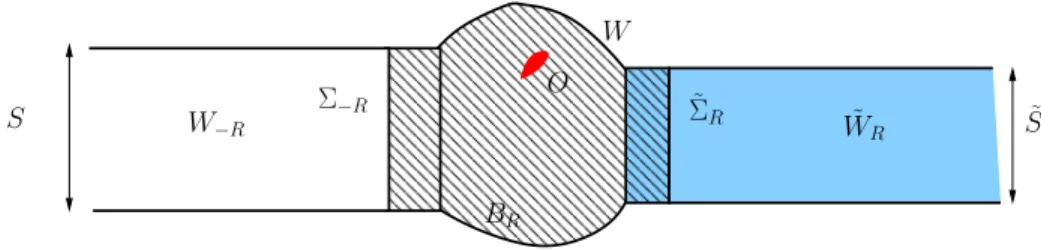
As mentioned in the introduction, in order to image a weld bead, we consider a transition zone between two half-waveguides. The domain W now consists of three domains, a left half-waveguide W_´R“ S ˆ p´8, ´Rq, a right half-waveguide

W´R W˜R S˜ O W BR ˜ ΣR S Σ´R

Figure 3: A waveguide with a transition zone (the domain BR is hatched)

˜

WR“ ˜S ˆ pR, `8q and a bounded domain BR in between, the transverse section

Σ´R “ S ˆ t´Ru separating the domains W´R and BR, the transverse section

˜

ΣR“ ˜S ˆ tRu separating the domains BR and ˜WR. It should be noted (see Figure

3) that the domain BRcontains a finite part of the half-waveguides WR0 and ˜W´R0,

R0ă R. The refractive index η P L8pW q is again constant in W´R0 and in ˜WR0,

with ηpxq “ 1 for x P W´R0 and ηpxq “ ˜n for x P ˜WR0. This in particular implies

that ηpxq “ 1 for x P W´R and ηpxq “ ˜n for x P ˜WR. For this waveguide W with a

junction, for n P N we can as previously define g`

n,0 as the extension of g`n in W´R

by 0 in BRY ˜WR and ˜gn,0´ as the extension of ˜g´n in ˜WR by 0 in BRY W´R. We

now introduce the reference fields un and ˜un defined by problems (5) and (6) for

n P N and the fundamental solution Gp¨, yq defined by problem (17) for y P W . If the point y belongs to a straight part of the domain W , we have simple expressions for Gp¨, yq in terms of the reference fields.

Proposition 9. The fundamental solution Gp¨, yq has the following properties: • for y P W´R and x P W with x3ą ´R,

Gpx, yq “ ´ÿ nPN 1 2iβn g´ npyqunpxq,

• for y P ˜WR and x P W with x3ă R,

Gpx, yq “ ´ÿ nPN 1 2i ˜βn ˜ g` npyq˜unpxq,

where un and ˜un are the solutions to problems (5) and (6), respectively.

Proof. The proof is very close to the one of Proposition 3. We only consider the case when y P W´R and x P W with x3ą ´R (the other case is similar). We again

use the decomposition Gp¨, yq “ G0p¨, yq ` Gsp¨, yq, where G0p¨, yq is the extension

of Gp¨, yq in W´R by 0 in BRY ˜WR. The field Gsp¨, yq satisfies the transmission

problem $ ’ ’ ’ ’ ’ ’ ’ ’ ’ ’ ’ & ’ ’ ’ ’ ’ ’ ’ ’ ’ ’ ’ % ∆Gsp¨, yq ` k2η2Gsp¨, yq “ 0 in W´RY BRY ˜WR BνGsp¨, yq “ 0 on BW JG s p¨, yqK “ G p¨, yq on Σ´R JBx3G s p¨, yq_{K “ B}x3Gp¨, yq on Σ´R JG s p¨, yqK “ 0 on Σ˜R JBx3G s p¨, yqK “ 0 on Σ˜R Gsp¨, yq is outgoing. (34)

We now use the decomposition un “ g`n,0` v s

n for all n P N. The field v s

n satisfies

the transmission problem $ ’ ’ ’ ’ ’ ’ ’ ’ ’ ’ ’ ’ & ’ ’ ’ ’ ’ ’ ’ ’ ’ ’ ’ ’ % ∆v_ns` k2η2v<sub>n</sub>s “ 0 in W´RY BRY ˜WR Bνvns “ 0 on BW Jv s nK “ g ` n on Σ´R JBx3v s nK “ Bx3g ` n on Σ´R Jv s nK “ 0 on Σ˜R JBx3v s nK “ 0 on Σ˜R vnsp¨, yq is outgoing. (35) Since x3ą y3 we have Gpx, yq “ ´ÿ nPN 1 2iβn g´ npyqg`npxq,

which in view of the systems (34) and (35) implies that Gs px, yq “ ´ÿ nPN 1 2iβn g´ npyqv s npxq.

We complete the proof observing that in BRY ˜WR, we have gn,0` “ 0 and G0p¨, yq “ 0,

that is un“ vsn and Gp¨, yq “ Gsp¨, yq.

Remark 5. We note that in contrast with Proposition 3, a closed-form expression for Gpx, yq is not given in Proposition 9 for all px, yq P W ˆ W .

We now introduce an obstacle within the domain W , more precisely in BR,

de-noting again Ω “ W zO. Once again we define the solutions up¨, yq and usp¨, yq to problems (22) and (23), for all y P Ω. We also introduce the operators N and H defined by (24) and (25). Then Theorem 2.1, Lemma 2.2 and Proposition 6 still hold (in particular, Lemma 2.2 is now a consequence of Proposition 9). However, Proposition 7 is not valid any more. Using again the reciprocity relationship satis-fied by the fundamental solution G, we get the following proposition, which is the analogous of Proposition 8.

Proposition 10. For x P Σ´R and z P BR,

Gpx, zq “ ´ ÿ mPN eiβmR 2iβm umpzqθmpxSq, for x P ˜ΣR and z P BR, Gpx, zq “ ´ ÿ mPN ei ˜βmR 2i ˜βm ˜ umpzq˜θmpxSq,

By restricting the series to P or ˜P terms, in the full-scattering case the near-field equation N ˆh “ Gp¨, zq|_Σˆ now amounts to the finite system

ˆA´ _A˜´ A` <sub>A</sub>˜` ˙ ˆH´ H` ˙ “ˆD ´<sub>pzq</sub> D`_pzq ˙ ,

where the matrices A´_{, ˜A}´_{, A}`<sub>and ˜A</sub>`_{are given by (27), the vectors H}´ _{and H}`

are given by (28), and the vectors D´_{pzq and D}`_{pzq are given by (31) and (32),}

respectively. In the back-scattering case, the near-field equation N ˆh “ Gp¨, zq|_Σˆ

reduces to the finite system

A´H´“ D´pzq.

4

Extension to a junction of several half-waveguides

In the previous section we have addressed the Linear Sampling Method to image a junction between two half-waveguides. In the present section we wish to extend such method to a junction of a finite number M of half-waveguides. Since the jus-tifications are the same as for the case M “ 2, we skip them. However we have to introduce some notations. The union of the junction and all half-waveguides is de-noted W and is characterized by a refractive index η P L8_{pW q. Each half-waveguide}

Wj_{, j “ 0, . . . , M ´ 1, has a constant section S}j _{and a constant refractive index}

ηj_{. We introduce the eigenvalues and eigenfunctions pλ}j

n, θnjqnPN of the transverse

problem (2) associated to the section Sj_{of half-waveguide W}j_{. Denoting κ}j

“ kηj, the corresponding wave numbers βj

n are computed following (3) by replacing κ by

κj _{and λ}

n by λjn. The junction is a bounded domain B such that

W “ B Y

M ´1

ď

j“0

Wj.

Each half-waveguide Wj _{has its own local set of coordinates x “ px}

S, x3q, where

x3 is oriented from infinity to the junction, so that Wj “ Sjˆ p´8, ´Rjq. The

support of emitters and receivers, again denoted ˆΣ, is defined by ˆ Σ “ M ´1 ź j“0 Σj,

where Σj _{is the transverse section of the half-waveguide W}j _{of local coordinate}

x3“ ´Rj. Some of the previous notations are illustrated on figure 4 for M “ 3. For

j “ 0, . . . , M ´ 1 and n P N, the guided mode gj

nwhich propagates or exponentially

decreases in the half-waveguide Wj from infinity to the junction satisfies

gj_npxq “ eiβjnx3_θj

npxSq.

The number of propagating modes in the half-waveguide Wj is denoted P pjq. To

each of such guided mode gj

n we can associate a reference field ujn via problem

(5), by replacing g`

n by gnj. Similarly, for any y P W we define the fundamental

solution Gp¨, yq via problem (17). Let us now assume that there is a Dirichlet obstacle O to retrieve in the junction B. For all y P W , we introduce the total field

B

W

W

W

Σ

Σ

Σ

W

O

Figure 4: A junction of three half-waveguides (the domain B is hatched)

up¨, yq which satisfies (22) and the scattered field us

p¨, yq which satisfies (23) with f “ ´Gp¨, yq|BO. For j “ 0, . . . , M ´ 1 and n P N, the solution to the problem (23)

for f “ ´uj

n|BO is denoted us,jn . The near-field equation in the full-scattering case

is: for each z PG , which is a sampling grid of B, find ˆh P ˆΣ such that ˆż

ˆ Σ

usp¨, yqˆhpyq dspyq ˙

ˇ ˇ_ˆ

Σ“ Gp¨, zq|Σˆ.

In what follows, the index e refers to the emitter, the index r to the receiver. The above near-field equation also reads: for r “ 0, . . . , M ´ 1 and x P Σr _find

ph0, h1_{, . . . , h}M ´1_{q P Σ}0 ˆ Σ1ˆ . . . ˆ ΣM ´1such that M ´1 ÿ e“0 ż Σe

uspx, yqhepyq dspyq “ Gpx, zq. (36)

Let us give some explicit expression of the left-hand side of the near-field equation (36). By proceeding as in Lemma 2.2, for y P Σe_{and x P B, we get}

uspx, yq “ ´ÿ nPN eiβe nRe 2iβe n us,en pxqθnepySq,

which by denoting for e, r “ 0, . . . , M ´ 1 and n P N, us,e_n |Σr“ ÿ mPN pUneq r mθ r m and h e “ ÿ mPN he_mθ_me,

implies that for r “ 0, . . . , M ´ 1 and x P Σr_, M ´1

ÿ

e“0

ż

Σe

uspx, yqhepyq dspyq “ ´

M ´1 ÿ e“0 ÿ mPN ÿ nPN eiβe_nRe 2iβe n pUneq r mh e nθ r mpxSq.

Let us now give an explicit expression of the right-hand side of (36). For r “ 0, . . . , M ´ 1 and x P Σr, for all z PG , using again the reciprocity relationship we get Gpx, zq “ Gpz, xq “ ´ ÿ mPN eiβ_mrRr 2iβr m ur_mpzqθrmpxSq.

Finally, if we restrict the series to the number of propagating modes in each half-waveguide, we obtain the following discrete near-field equation: for r “ 0, . . . , M ´1, for m “ 0, . . . , P prq ´ 1, M ´1 ÿ e“0 P peq´1 ÿ n“0 eiβe nRe 2iβe n pUneq r mh e n“ eiβr mRr 2iβr m ur_mpzq. (37)

Remark 6. From the system (37), which corresponds to the full-scattering data, it is very easy to deduce the one obtained for partial data, that is when emitters and receivers are located on strictly less than M transverse sections Σj_.

5

Numerical experiments

5.1

Introduction

In order to show some 2D numerical experiments of the inverse problem, we compute artificial data by solving the forward scattering problems (23) in a bounded domain with the help of Dirichlet-to-Neumann operators on each half-waveguide and by using a Finite Element Method. This enables us to construct the matrices A´_,

A`<sub>, ˜A</sub>´ <sub>and ˜A</sub>` _{defined by (27) and the corresponding matrices in the case of the}

extension to a junction of several half-waveguides (see the left-hand side of (37)). In all the experiments conducted in the sequel, the identification results are presented for exact data (the data are exactly the scattered fields obtained by the FEM) and for noisy data. Noisy data are obtained following the method described in [3]. Indeed, let us consider the trace on a transverse section Σ of a scattered field us

obtained with the FEM. We compute, with the help of a subdivision of Σ into a finite number of intervals, a pointwise Gaussian noise b. The noisy data us

δ is then

defined on Σ by

us_δ“ us` α b,

where the real number α ą 0 is calibrated in such a way that }us_δ´ us}L2_pΣq“ 0.1 }us}_L2_pΣq,

which means that our relative amplitude of noise is 10%. For z PG , let us denote

AH “ Dpzq (38)

either the pP ` ˜P q ˆ pP ` ˜P q full-scattering system (26) or the P ˆ P back-scattering system (33) for a junction of two half-waveguides. In the case of exact data A, we exactly solve (38). In the presence of noisy data Aδ, with ~Aδ´ A~ ď δ, where ~¨~

is a matrix norm, we solve the Tikhonov equation associated with (38), that is

where A˚

δ is the adjoint of Aδ and ε ą 0. Following exactly [22] and as in [3],

for a given point z, the regularization parameter ε is uniquely determined as a function of δ according to the Morozov’s discrepancy principle. More precisely, we compute ε by using a singular value decomposition of Aδ and a simple dichotomy

method. It remains to construct the right-hand side of (26), or (37) in the case of the extension to a junction of several half-waveguides. This is done by using formulas (31) and (32), which require to compute the reference fields un and ˜un

(they satisfy (5) and (6)) and the corresponding fields in the case of the extension to a junction of several half-waveguides (see the right-hand side of (37)). Unless we consider a straight waveguide (see Proposition 4), these reference fields have to be computed numerically by using a FEM. A crucial point is that those reference fields are independent of z and of the obstacle O. They are hence computed once and for all, which is important as regards the efficiency of the Linear Sampling Method in this context. In comparison with the case of a straight and homogeneous waveguide, the computational cost is increased by the preliminary FEM computations of the reference fields, in particular if the junction domain is large. In all the pictures presented hereafter, we show the level sets of the function

ψpzq “ log ˆ 1 }Hpzq} ˙ ,

where Hpzq is the solution to (38) for exact data and the solution to (39) for noisy data, such solution depending implicitly on z. Here } ¨ } denotes a L2_{discrete norm.}

In view of Theorem 2.1, ψpzq is almost ´8 unless z P O, which means that the level sets of ψ almost characterize the obstacle.

5.2

Waveguide with an abrupt change of refractive index

We consider the particular case of section 2 when the waveguide is straight, that is S “ ˜S, but characterized by an abrupt change of refractive index, that is κ ‰ ˜κ. Here we have h “ ˜h “ 1, while R “ 1. We consider four kinds of obstacle.

1. A square within the left half-waveguide W0.

2. A circle within the right half-waveguide ˜W0.

3. The union of the two previous obstacles.

4. A triangle at the interface of half-waveguides W0and ˜W0.

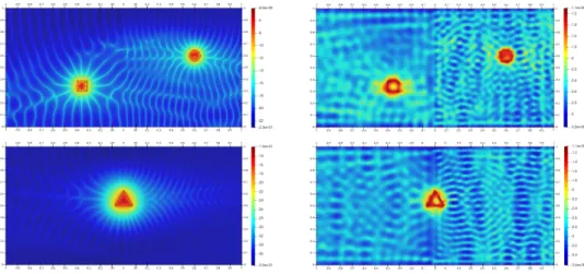
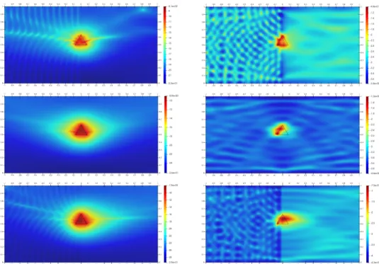
In figure 5, we show the identification result for obstacle 3 and obstacle 4 in the full-scattering case, with wave number κ “ 40 in the left half-waveguide W0 and

˜

κ “ 60 in the right half-waveguide ˜W0. The corresponding number of propagating

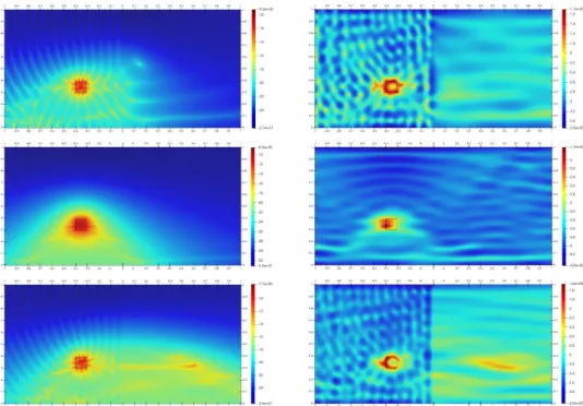
modes are P “ 13 and ˜P “ 20, respectively. We observe that the quality of the images are as good as if the waveguide were homogeneous. Next, in figures 6, 7 and 8, we present the identification results in the back-scattering case for obstacle 1 (obstacle in the half-waveguide which supports the data), obstacle 2 (obstacle in the half-waveguide which does not support the data) and obstacle 4 (obstacle at the interface), respectively. For each of these obstacles, we show the obtained images when pκ, ˜κq “ p40, 20q, pκ, ˜κq “ p40, 40q and pκ, ˜κq “ p40, 60q. We can draw two kinds of conclusion. Firstly, as expected the obstacle is better retrieved when it is located in the half-waveguide which supports the data because the identification

Figure 5: Full-scattering, κ “ 40 (P “ 13) and ˜κ “ 60 ( ˜P “ 20). Top left: obstacle 3 and exact data. Top right: obstacle 3 and noisy data. Bottom left: obstacle 4 and exact data. Bottom right: obstacle 4 and noisy data.

benefits from the reflected waves by the interface between the two half-waveguides. Secondly, in the case when the obstacle lies in the half-waveguide which does not support the data, we observe that the obstacle is not better retrieved if ˜κ is larger than κ instead of being equal to κ. This could seem paradoxical, in the sense that the larger is the wave number, the bigger is the number of propagating modes and hence the better should be the resolution. This can be interpreted, in view of Proposition 4, as follows: the P propagating modes g`

n in W0 are transmitted in

˜

W0 in the form of the modes ˜g`n, so that only P propagating modes in ˜W0among

their total number ˜P ą P are excited, the remainder p ˜P ´ P q are not.

5.3

Waveguide with an abrupt change of section

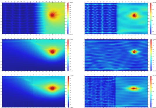
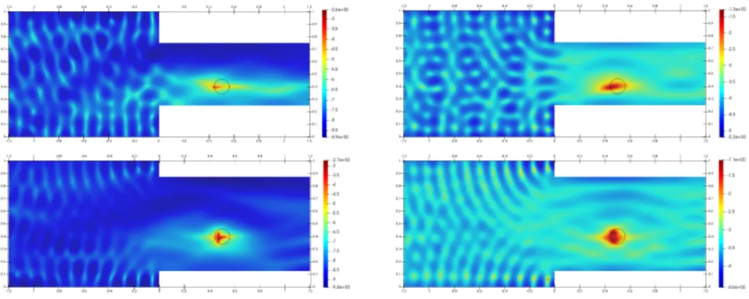
We now consider the particular case of section 2 when the refractive index is uniform, that is κ “ ˜κ, but the waveguide is characterized by an abrupt change of section, that is S ‰ ˜S. In figure 9, we show the identification result for obstacle 3 in the full-scattering case, with κ “ ˜κ “ 40, but h ‰ ˜h, that is h “ 0.65 and ˜h “ 1. The corresponding numbers of propagating modes are P “ 9 and ˜P “ 13. Again we observe that the quality of the images are as good as if the waveguide were straight. Now we consider the back-scattering case when the obstacle lies in the half-waveguide which supports the data (obstacle 1), in the particular case h{˜h ą 1 in figure 10 and h{˜h ă 1 in figure 11. The interpretation of these results is quite clear. For h “ 1, the identification results are better if ˜h “ 0.5 than if ˜h “ 0.75 (figure 10), because the amount of reflected waves at the interface between the two half-waveguides is larger (at the limit when ˜h tends to 0, our waveguide tends to a terminating waveguide like in [13], which can be seen as an ideal situation). On the contrary, for ˜h “ 1, the identification results are better if h “ 0.75 than if h “ 0.5 (figure 11), because the number of incident propagating modes in W0 is larger in

the first case. Next we consider the back-scattering case when the obstacle lies in the half-waveguide which does not support the data (obstacle 2), in the particular case h{˜h ą 1 in figure 12 and h{˜h ă 1 in figure 13. For h “ 1, the identification

Figure 6: Back-scattering for obstacle 1. Top left: κ “ 40 (P “ 13) and ˜κ “ 20 ( ˜P “ 7), exact data. Top right: κ “ 40 and ˜κ “ 20, noisy data. Middle left: κ “ ˜κ “ 40 (P “ ˜P “ 13), exact data. Middle right: κ “ ˜κ “ 40, noisy data. Bottom left: κ “ 40 (P “ 13) and ˜κ “ 60 ( ˜P “ 20), exact data. Bottom right: κ “ 40 and ˜κ “ 60, noisy data.

results are better if ˜h “ 0.75 than if ˜h “ 0.5 (figure 12), because the amount of reflected waves increases while the amount of transmitted waves that reach the obstacle decreases, which deteriorates the quality of the identification. For ˜h “ 1, the identification results are better if h “ 0.75 than if h “ 0.5 (figure 13), because the number of incident propagating modes in W0is larger in the first case, and they

are all transmitted in the form of propagating modes in ˜W0 because ˜P ą P .

5.4

Junction of three waveguides

To complete the numerical experiments, we present some identification results in the case of a junction of three half-waveguides presented in section 4 (see figure 4, which shows the position of the three half-waveguides), the Dirichlet obstacle being kite-shaped. The thickness of the three half-waveguides W0_{, W}1 _{and W}2 _are

h0 _{“ 1, h}1 _{“ 1.2 and h}2 _{“ 0.9, respectively. The junction is a disk of radius 0.8,}

while the three transverse sections Σ0, Σ1and Σ2 are located at the same distance Rj “ 3 (j “ 0, 1, 2) of the center of such disk. The refractive index is η “ 1 in the whole waveguide, while k “ 40, which implies that the number of propagating modes in each half-waveguide is P p0q “ 13, P p1q “ 16 and P p2q “ 12, respectively. The figure 14 represents the obstacle which is retrieved when the emitters and receivers are located on a single transverse section Σj _{of a single half-waveguide}

Figure 7: Back-scattering for obstacle 2. Top left: κ “ 40 (P “ 13) and ˜κ “ 20 (P “ 7), exact data. Top right: κ “ 40 and ˜κ “ 20, noisy data. Middle left: κ “ ˜κ “ 40 (P “ ˜P “ 13), exact data. Middle right: κ “ ˜κ “ 40, noisy data. Bottom left: κ “ 40 (P “ 13) and ˜κ “ 60 ( ˜P “ 20), exact data. Bottom right: κ “ 40 and ˜κ “ 60, noisy data.

one hand when the emitters and receivers are located on the two transverse sections Σ0 _{and Σ}1 _{of the half-waveguides W}0 _{and W}1_{, on the other hand when they are}

located on all the transverse sections Σj _{of all half-waveguides W}j_{, for j “ 0, 1, 2.}

Unsurprisingly, with or without noise, the larger is the set of data, the better is the identification.

6

Conclusions

The numerical results of the previous section seem to prove that a sampling method such as the Linear Sampling Method can be extended to the case of a junction of several half-waveguides. Some extensions in several directions could be envisioned. Firstly, our method could be extended to elasticity, which is necessary in the context of ultrasonic Non Destructive Testing, as in [9]. Secondly, in the context of NDT, for obvious reasons emitters and receivers cannot be located on transverse sections, but only on the boundary of the waveguide. We can cope with this problem by proceeding as in [7] (acoustics) and in [9] (elasticity), where it is shown that, starting from boundary data, we can come back to data on transverse sections by inverting some emission and reception matrices, the distance between the sensors and their number playing a crucial role in the conditioning of those matrices (see [7]). Lastly, the present article is restricted to the case of Dirichlet obstacles. The generalization

Figure 8: Back-scattering for obstacle 4. Top left: κ “ 40 (P “ 13) and ˜κ “ 20 ( ˜P “ 7), exact data. Top right: κ “ 40 and ˜κ “ 20, noisy data. Middle left: κ “ ˜κ “ 40 (P “ ˜P “ 13), exact data. Middle right: κ “ ˜κ “ 40, noisy data. Bottom left: κ “ 40 (P “ 13) and ˜κ “ 60 ( ˜P “ 20), exact data. Bottom right: κ “ 40 and ˜κ “ 60, noisy data.

Figure 9: Full-scattering, obstacle 3, κ “ ˜κ “ 40, h “ 0.65 (P “ 9) and ˜h “ 1 ( ˜P “ 13). Left: exact data. Right: noisy data.

to other types of obstacles is not an issue, for example Neumann obstacles or cracks, following [5] for acoustics and [19] for elasticity.

Acknowledgments

Figure 10: Back-scattering for obstacle 1, κ “ ˜κ “ 30 and h ą ˜h. Top left: h “ 1 (P “ 10) and ˜h “ 0.5 ( ˜P “ 5), exact data. Top right: h “ 1 and ˜h “ 0.5, noisy data. Bottom left: h “ 1 (P “ 10) and ˜h “ 0.75 ( ˜P “ 8), exact data. Bottom right: h “ 1 and ˜h “ 0.75, noisy data.

Figure 11: Back-scattering for obstacle 1, κ “ ˜κ “ 30 and h ă ˜h. Top left: h “ 0.5 (P “ 5) and ˜h “ 1 ( ˜P “ 10), exact data. Top right: h “ 0.5 and ˜h “ 1, noisy data. Bottom left: h “ 0.75 (P “ 8) and ˜h “ 1 ( ˜P “ 10), exact data. Bottom right: h “ 0.75 and ˜h “ 1, noisy data.

References

[1] D. Colton and A. Kirsch A simple method for solving inverse scattering prob-lems in the resonance region, Inverse Probprob-lems, 12,4 (1996), 383–393. [2] F. Cakoni, D. Colton “Qualitative Methods In Inverse Scattering Theory”

Springer-Verlag, Berlin, 2006.

[3] L. Bourgeois and E. Lun´eville The linear sampling method in a waveguide: a modal formulation, Inverse Problems, 24,1 (2008), 015018, 20 pp.

[4] L. Bourgeois, F. Le Lou¨er and E. Lun´eville On the use of Lamb modes in the linear sampling method for elastic waveguides, Inverse Problems, 27,5 (2011), 055001, 27 pp.

Figure 12: Back-scattering for obstacle 2, κ “ ˜κ “ 30 and h ą ˜h. Top left: h “ 1 (P “ 10) and ˜h “ 0.5 ( ˜P “ 5), exact data. Top right: h “ 1 and ˜h “ 0.5, noisy data. Bottom left: h “ 1 (P “ 10) and ˜h “ 0.75 ( ˜P “ 8), exact data. Bottom right: h “ 1 and ˜h “ 0.75, noisy data.

Figure 13: Back-scattering for obstacle 2, κ “ ˜κ “ 30 and h ă ˜h. Top left: h “ 0.5 (P “ 5) and ˜h “ 1 ( ˜P “ 10), exact data. Top right: h “ 0.5 and ˜h “ 1, noisy data. Bottom left: h “ 0.75 (P “ 8) and ˜h “ 1 ( ˜P “ 10), exact data. Bottom right: h “ 0.75 and ˜h “ 1, noisy data.

[5] L. Bourgeois and E. Lun´eville On the use of the linear sampling method to identify cracks in elastic waveguides, Inverse Problems, 29,2 (2013), 025017, 19 pp.

[6] L. Bourgeois and S. Fliss On the identification of defects in a periodic waveguide from far field data, Inverse Problems, 30,9 (2014), 095004, 31 pp.

[7] V. Baronian, L. Bourgeois and A. Recoquillay Imaging an acoustic waveguide from surface data in the time domain, Wave Motion, 66 (2016), 68–87. [8] P. Monk and V. Selgas An inverse acoustic waveguide problem in the time

Figure 14: Data on a single half-waveguide. Top left: exact data on section Σ0. Top right: noisy data on section Σ0. Middle left: exact data on section Σ1. Middle right: noisy data on section Σ1_{. Bottom left: exact data on section Σ}2_{. Bottom}

right: noisy data on section Σ2_.

[9] V. Baronian, L. Bourgeois, B. Chapuis and A. Recoquillay Linear sampling method applied to non destructive testing of an elastic waveguide: theory, nu-merics and experiments, Inverse Problems, 34,7 (2018), 075006, 34 pp. [10] A. Charalambopoulos, D. Gintides, K. Kiriaki and A. Kirsch The factorization

method for an acoustic wave guide, in “Mathematical methods in scattering theory and biomedical engineering”, World Sci. Publ., Hackensack, NJ, (2006), 120–127.

[11] C. Tsogka, D. A. Mitsoudis and S. Papadimitropoulos Selective imaging of extended reflectors in two-dimensional waveguides, SIAM J. Imaging Sci., 6,4

Figure 15: Top: data on two half-waveguides. Left: exact data on sections Σ0 and Σ1. Right: noisy data on sections Σ0 and Σ1. Bottom: data on three half-waveguides. Left: exact data on sections Σ0, Σ1 and Σ2. Right: noisy data on sections Σ0, Σ1 and Σ2.

(2013), 2714–2739.

[12] C. Tsogka, D. A. Mitsoudis and S. Papadimitropoulos Partial-aperture array imaging in acoustic waveguides, Inverse Problems, 32,12 (2016), 125011, 31pp. [13] C. Tsogka, D. A. Mitsoudis and S. Papadimitropoulos Imaging extended reflec-tors in a terminating waveguide, SIAM J. Imaging Sci., 11,2 (2018), 1680–1716. [14] L. Borcea, F. Cakoni and S. Meng A direct approach to imaging in a waveguide

with perturbed geometry, J. Comput. Phys., 392 (2019), 556–577.

[15] L. Borcea and S. Meng Factorization method versus migration imaging in a waveguide, Inverse Problems, 35,12 (2019), 0124006, 33 pp.

[16] L. Borcea and S. Meng Imaging with electromagnetic waves in terminating waveguides, Inverse Probl. Imaging, 10,4 (2016), 915–941.

[17] P. Monk, V. Selgas and F. Yang Near-field linear sampling method for an in-verse problem in an electromagnetic waveguide, Inin-verse Problems, 35,6 (2019), 065001, 27 pp.

[18] A.-S. Bonnet-Bendhia and A. Tillequin A generalized mode matching method for scattering problems with unbounded obstacles, Journal of Computational Acoustics, 9,4 (2001), 1611–1631.

[19] L. Bourgeois and E. Lun´eville On the use of sampling methods to identify cracks in acoustic waveguides, Inverse Problems, 28,10 (2012), 105011, 18 pp. [20] L. Audibert, A. Girard and H. Haddar Identifying defects in an unknown back-ground using differential measurements, Inverse Probl. Imaging, 9,3 (2015), 625–643.

[21] L. Bourgeois and E. Lun´eville The linear sampling method in a waveguide: A formulation based on modes, Journal of Physics: Conference Series, 135 (2008), 012023.

[22] D. Colton, M. Le Piana and R. Potthast A simple method using Morozov’s discrepancy principle for solving inverse scattering problems, Inverse Problems, 13,6 (1997), 1477–1493.