HAL Id: hal-00436671
https://hal.archives-ouvertes.fr/hal-00436671
Submitted on 5 Jan 2016
HAL is a multi-disciplinary open access
archive for the deposit and dissemination of
sci-entific research documents, whether they are
pub-lished or not. The documents may come from
teaching and research institutions in France or
abroad, or from public or private research centers.
L’archive ouverte pluridisciplinaire HAL, est
destinée au dépôt et à la diffusion de documents
scientifiques de niveau recherche, publiés ou non,
émanant des établissements d’enseignement et de
recherche français ou étrangers, des laboratoires
publics ou privés.
responses to ENSO inferred from an ensemble of
Chemistry Climate Models
Chiara Cagnazzo, Elisa Manzini, Natalia Calvo, A. Douglass, H. Akiyoshi,
Slimane Bekki, M. Chipperfield, M. Dameris, M. Deushi, A. M. Fischer, et al.
To cite this version:
Chiara Cagnazzo, Elisa Manzini, Natalia Calvo, A. Douglass, H. Akiyoshi, et al.. Northern winter
stratospheric temperature and ozone responses to ENSO inferred from an ensemble of Chemistry
Climate Models. Atmospheric Chemistry and Physics, European Geosciences Union, 2009, 9 (22),
pp.8935-8948. �10.5194/acp-9-8935-2009�. �hal-00436671�
www.atmos-chem-phys.net/9/8935/2009/ © Author(s) 2009. This work is distributed under the Creative Commons Attribution 3.0 License.
Chemistry
and Physics
Northern winter stratospheric temperature and ozone responses to
ENSO inferred from an ensemble of Chemistry Climate Models
C. Cagnazzo1, E. Manzini1,2, N. Calvo3, A. Douglass4, H. Akiyoshi5, S. Bekki6, M. Chipperfield7, M. Dameris8, M. Deushi9, A. M. Fischer10,*, H. Garny8, A. Gettelman11, M. A. Giorgetta12, D. Plummer13, E. Rozanov10,15, T. G. Shepherd14, K. Shibata9, A. Stenke8, H. Struthers16,**, and W. Tian7
1Centro Euro-Mediterraneo per i Cambiamenti Climatici, Bologna, Italy 2Istituto Nazionale di Geofisica e Vulcanologia, Bologna, Italy
3Dpto. Fisica de la Tierra II, Universidad Complutense de Madrid, Spain 4NASA Goddard Space Flight Center, Greenbelt MD, USA
5National Institute for Environmental Studies, Tsukuba, Japan 6Service d’Aeronomie du CNRS, IPSL, Paris, France
7School of Earth and Environment, University of Leeds, Leeds, UK 8DLR-Institut f¨ur Physik der Atmosph¨are, Oberpfaffenhofen, Germany 9Meteorological Research Institute, Tsukuba, Ibaraki 305-0052, Japan
10Institute for Atmospheric and Climate Science, ETH Z¨urich, Z¨urich, Switzerland 11National Center for Atmospheric Research, Boulder, Colorado, USA
12Max Planck Institute for Meteorology, Hamburg, Germany 13Environment Canada, Toronto, Ontario, Canada
14Department of Physics, University of Toronto, Toronto, Ontario, Canada
15Physical-Meteorological Observatory/World Radiation Center, Davos, Switzerland 16National Institute of Water & Atmospheric Research, Auckland, New Zealand
*now at: Federal Office of Meteorology and Climatology MeteoSwiss, Z¨urich, Switzerland **now at: ITM – Stockholms universitet, Stockholms, Sweden
Received: 10 April 2009 – Published in Atmos. Chem. Phys. Discuss.: 15 May 2009
Revised: 19 November 2009 – Accepted: 20 November 2009 – Published: 27 November 2009
Abstract. The connection between the El Ni˜no Southern
Oscillation (ENSO) and the Northern polar stratosphere has been established from observations and atmospheric model-ing. Here a systematic inter-comparison of the sensitivity of the modeled stratosphere to ENSO in Chemistry Climate Models (CCMs) is reported. This work uses results from a number of the CCMs included in the 2006 ozone assessment. In the lower stratosphere, the mean of all model simulations reports a warming of the polar vortex during strong ENSO events in February–March, consistent with but smaller than the estimate from satellite observations and ERA40 reanal-ysis. The anomalous warming is associated with an anoma-lous dynamical increase of column ozone north of 70◦N that is accompanied by coherent column ozone decrease in the
Correspondence to: C. Cagnazzo
Tropics, in agreement with that deduced from the NIWA col-umn ozone database, implying an increased residual circula-tion in the mean of all model simulacircula-tions during ENSO. The spread in the model responses is partly due to the large inter-nal stratospheric variability and it is shown that it crucially depends on the representation of the tropospheric ENSO tele-connection in the models.
1 Introduction
The El Ni˜no Southern Oscillation (ENSO) is a tropical atmosphere-ocean phenomenon and a source of large-scale climate variability for the atmosphere – ocean system. Dur-ing boreal winter, the typical teleconnection between the warm phases of ENSO and the mid-latitude North Pacific re-gion (Hoerling et al., 1997; Strauss and Shukla, 2000 among others) can favour the enhancement of mid-latitude planetary
waves and consequently their upward propagation into the stratosphere (Manzini et al., 2006). Due to this increase in extra-tropical stratospheric planetary wave activity, warm ENSO events have been found to be associated with anoma-lous warming and anomaanoma-lously high geopotential height in the polar stratosphere, both from observations (van Loon and Labitzke, 1987; Hamilton, 1993; Camp and Tung, 2007; Garfinkel and Hartmann, 2007) and comprehensive mod-eling of the troposphere-stratosphere system (Sassi et al., 2004; Taguchi and Hartmann, 2006; Manzini et al., 2006; Garcia-Herrera et al., 2006). Recently, the warm ENSO sig-nal in the Arctic has also been found in radiosonde data (Free and Seidel, 2009). At high Northern latitudes, large zonal mean anomalies, in temperature and zonal wind, as-sociated with the warm phase of ENSO appear in the upper stratosphere in early winter and then propagate downwards to the lower stratosphere on monthly time scales through wave mean flow interaction (Manzini et al., 2006). The model-ing work of Manzini et al. (2006) has shown that these zonal mean anomalies associated with ENSO occur also in the tro-posphere in late winter and spring, and the subsequent mod-eling work of Cagnazzo and Manzini (2009) has shown that they are implicated in the surface teleconnection between ENSO and the North European region.
Given that the reported polar warming associated with warm ENSO events is a manifestation of an enhanced Brewer-Dobson circulation, more ozone should be trans-ported from the source region in the tropics toward high po-lar latitudes during warm ENSO events. In fact, interannual variations in column ozone and temperature in the northern polar stratosphere are linked to planetary scale wave activity (Fusco and Salby, 1999; Randel et al., 2002; Weber et al., 2003). At Arctic and mid-latitude sites, an anomalous accu-mulation of column ozone was indeed reported for the strong and long lasting 1940–1942 ENSO event by Br¨onnimann et al. (2004). In the tropics, a signal in stratospheric ozone has been reported from the SAGE II satellite dataset (Randel et al., 2009). Consistently with the ENSO signal in ozone, Ran-del et al. (2009) and the independent work of Free and Sei-del (2009) report also an ENSO signal in the tropical lower stratosphere temperature.
The response to ENSO has also been analysed in a few Chemistry Climate Models (Fischer et al., 2008; Steinbrecht et al., 2006, Br¨onnimann et al., 2006; Garny et al., 2009; Randel et al., 2009) and in a chemical transport model (Sassi et al., 2004).
The purpose of this work is to extend these previous stud-ies that analyzed the ENSO response in Chemistry Climate Models (CCMs), by systematically evaluating the response to warm ENSO in the pool of simulations for the recent past performed with the CCMs participating in the Chemistry-Climate Model Validation Activity (CCMVal-1) of SPARC that are discussed in Eyring et al. (2006). Many of these mod-els contributed to the 2006 ozone assessment (WMO/UNEP, 2007). These simulations have been performed with
pre-scribed observed sea surface temperatures (SSTs), and there-fore include the ENSO forcing on the modeled atmosphere. However, the manifestation of the ENSO effect on the strato-sphere depends also on the ENSO teleconnection in the tro-posphere, not necessarily similarly represented in the CCMs. Another aspect obscuring the ENSO signal in the strato-sphere is the typical high variability of the boreal winter stratosphere.
The focus of this work is on the Northern polar strato-sphere temperature and ozone response during boreal winter, for the 1980–1999 period. Specifically, we aim at identify-ing any coherence in the temperature and ozone responses across the Chemistry Climate Models. This in turn may pro-vide some insight into understanding the causes of the range of responses, in terms of interannual variability and model biases.
Note that the cold ENSO events that occurred in the 1980– 1999 period have been found to have negligible influence on the Northern polar stratosphere during winter (Manzini et al., 2006; see also Sassi et al., 2004), and therefore are not considered in this work. The negligible response may be partly due to the smaller SST anomalies that occurred for cold events during the period considered here. This apparent little sensitivity of the Arctic stratosphere to cold ENSO de-rived from model results is consistent with the recent analysis of radiosonde temperature data by Free and Seidel (2009).
2 Datasets and methodology
2.1 Models
The CCM datasets used in this work result from transient runs aimed at reproducing the time period of 1980–1999 (Eyring et al., 2006): most of the simulations include an-thropogenic and natural forcings based on changes in SSTs, trace gases, solar variability, and aerosol effects (from major volcanic eruptions). The models are summarized and refer-enced in Table 1. The description of the external forcings can be found in Table 2 of Eyring et al. (2006).
Modeled monthly zonal mean temperature and column ozone and (when available) monthly three-dimensional geopotential height fields have been analyzed. AMTRAC, CCSRNIES, MRI, SOCOL and WACCM models have pro-vided a set of 3, 3, 5, 9 and 3 realizations (i.e., they have repeated the simulation of the 1980–1999 period with dif-ferent meteorological initial conditions), respectively. SO-COL, E39C-A and MRI models have provided outputs from updated model versions with respect to those de-scribed in Eyring et al. (2006). The analysis on the AM-TRAC, GEOSCCM, and 2 members of CCSRNIES simu-lations is restricted to the zonal mean fields, because three-dimensional fields were not available for these cases.
2.2 Observations and Reanalysis Data
Three datasets covering the 1980–1999 period, are consid-ered:
1. Time series of monthly mean temperature and geopo-tential height from the European Centre for Medium-Range Weather Forecast Re-Analysis (ERA-40, Uppala et al., 2005; Uppala et al., 2004).
2. Stratospheric Sounding Unit (SSU) temperatures (Nash and Edge, 1989; Brindley et al., 1999) and Mi-crowave Sounding Unit (MSU) temperatures (Spencer and Christy, 1995). These datasets consist of zonal temperature anomalies every 10 degrees from 70◦S to 70◦N for the 3 SSU channels (anomalies peaking at 15, 6, and 2 hPa) and 4 synthetic channels (peaking at 50, 20, 5, 1.5 and 0.5 hPa, Nash and Edge, 1989) and for the MSU channel (90 hPa).
3. NIWA column ozone dataset, which combines data from several United States and European satellites with a global set of ground stations (Bodeker et al., 2005).
2.3 Diagnostics
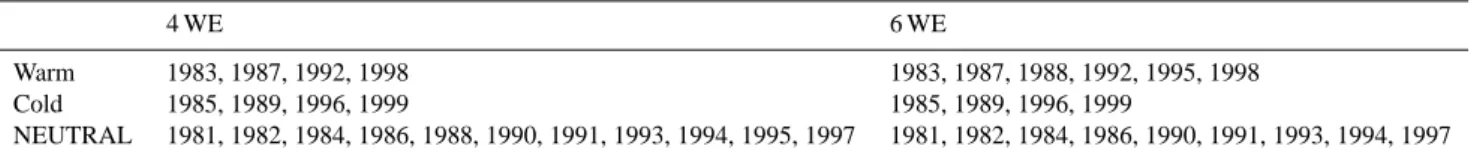
Composites for the period 1980–1999 are constructed for temperature, column ozone and eddy geopotential height fields. For each month of the extended winter season (Oc-tober to April), warm ENSO and NEUTRAL composites of monthly means are considered, for the models and the datasets. Our standard warm ENSO composite is made up of the 4 largest warm events that occurred in the period 1980–1999 (hereafter 4 WE), see Table 2 for the list of the events. The events are selected on the basis of the SST anomaly averaged from January to March in the Nino-3 re-gion from the National Centers for Environmental Predic-tion (NCEP)/Climate PredicPredic-tion Center (CPC) (http://www. cpc.ncep.noaa.gov/data/indices). These four events are those typically studied in climate research on ENSO teleconnec-tions, for example Strauss and Shukla (2000) and Manzini et al. (2006). Following Manzini et al. (2006), the NEUTRAL composite is made of the years within the 1980–1999 pe-riod, that exclude these warm ENSO events as well as the 4 largest cold ENSO events (see Table 2). Two of the four winters considered in the warm ENSO composite analysis were disturbed by volcanic eruptions (1982–1983 and 1991– 1992). Intense volcanic eruptions are believed to cause on average a cooling and a strengthening of the vortex (Lab-itzke and Van Loon, 1989) possibly leading to a distortion of the anomaly associated with ENSO in the polar strato-sphere. For this reason, a second warm ENSO composite has been constructed, including two additional ENSO events (hereafter 6 WE, see Table 2), with the two additional events not disturbed by the volcanic external forcing, albeit charac-terized by weaker ENSO phenomena.
Table 1. List of the models used in this work. AMTRAC (3) Austin et al. (2006)
Austin and Wilson (2006) CCSRNIES (3) Akiyoshi et al. (2004)
Kurokawa et al. (2005) Akiyoshi et al. (2009) CMAM Beagley et al. (1997)
de Grandpr´e et al. (2000) Scinocca et al. (2008) E39C-A Stenke et al. (2009)
Garny et al. (2009) GEOSCCM Bloom et al. (2005)
Stolarski et al. (2006) LMDZrepro Lefevre et al. (1994) MAECHAM4CHEM Manzini et al. (2003)
Steil et al. (2003)
MRI (5) Shibata and Deushi (2008a, b) SOCOL (9) Egorova et al. (2005)
Rozanov et al. (2005) UMETRAC Austin (2002)
Austin and Butchart (2003) Struthers et al. (2004) UMSLIMCAT Tian and Chipperfield (2005) WACCM (3) Garcia et al. (2007)
As discussed for volcanic eruptions, the QBO and solar cycle are sources of variability for the stratosphere and their non-linear interaction with the ENSO signal could interfere with the stratospheric response to ENSO (e.g. Garfinkel and Hartmann, 2007). As mentioned in Sect. 2.1, most of the CCMVal simulations include these signals. To investigate these connections in beyond the scope of this work, therefore the modeled stratospheric response to ENSO has not been stratified separating model simulations with and without one (or more) of these signals, an approach that would require a much larger ensemble of simulations.
For every field considered, “ENSO anomalies” are de-fined as the difference between the warm ENSO composite and the NEUTRAL composite.
In order to compactly compare the response of each model to the ENSO forcing, the following 4 indices are defined and calculated from the ENSO anomalies:
1T index, defined as the February–March, polar cap
(70◦N–90◦N) and 30–70 hPa average of the ENSO zonal mean temperature anomaly (<T >ENSO−<T >NEUTRAL).
This index represents the temperature anomaly associated to ENSO in the lower stratosphere at the end of win-ter/beginning of spring.
1Z index. The known tropospheric teleconnection of ENSO with Northern midlatitude stationary waves in December-January-February (DJF) consists of an eastward elongation of the North Pacific trough (Hoerling et al., 1997;
Table 2. Warm ENSO, cold ENSO and NEUTRAL years (year index for January) for 4 WE and 6 WE.
4 WE 6 WE
Warm 1983, 1987, 1992, 1998 1983, 1987, 1988, 1992, 1995, 1998
Cold 1985, 1989, 1996, 1999 1985, 1989, 1996, 1999
NEUTRAL 1981, 1982, 1984, 1986, 1988, 1990, 1991, 1993, 1994, 1995, 1997 1981, 1982, 1984, 1986, 1990, 1991, 1993, 1994, 1997
see their Fig. 6). In order to quantify this typical tropospheric pattern and to evaluate the troposphere of the models, we defined the 1Z index in the following way: At 50◦N and 500 hPa, for the DJF average: (1) The difference between the warm ENSO and the NEUTRAL ENSO composites, of the stationary eddy geopotential height is computed and de-fined to be the tropospheric stationary wave anomaly. (2) The minimum value of the tropospheric stationary wave anomaly between 180 and 360 longitude is searched and found. (3) This minimum value is smoothed by an average over 10% of its value. (4) The smoothed minimum of the tropospheric stationary wave anomaly multiplied by −1 is the 1Z index. The link between this index and the eddy heat flux at 100 hPa is discussed in the Appendix A.
1O3 index, defined as the February–March, polar cap
(70◦N–90◦N) average of the ENSO zonal mean column ozone anomaly (<O3>ENSO−<O3>NEUTRAL). This
in-dex is aimed at quantifying the column ozone anomaly asso-ciated to the ENSO teleconnection in February and March in the polar region only.
1O3(FM-ND) index, defined as the February–March
mean minus the November–December mean of an area av-erage of the ENSO zonal mean column ozone anomaly. This index has been calculated for the polar cap (70◦N–90◦N) and the tropics (15◦S–15◦N) ((<O3(FM)> − <O3(ND)> )ENSO−(<O3(FM)> − <O3(ND)>)NEUTRAL) and it
repre-sents the wintertime increase/decrease in the ENSO zonal mean column ozone anomaly at polar/tropical latitudes. Salby and Callaghan (2002) have shown that it is the ten-dency (i.e. the anomalous wintertime increase of column ozone at high latitudes) that is coupled to the residual cir-culation.
3 Temperature in the lower stratosphere
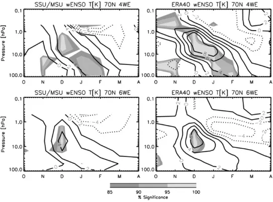
Figure 1 shows the time evolution from October to April of the ENSO zonal mean temperature anomalies at 70◦N, from 100 hPa to 0.1 hPa, for the composite of the 4 warm events (top) and the 6 warm events (bottom), for both the SSU/MSU (left) and ERA40 (right) data. Figure 1 shows that in the case of the 4 largest ENSO events, the polar warming oc-curs first in the upper stratosphere (about 4 K for SSU and 8 K for ERA40, significant in December at 95%) and then descends to the lower stratosphere, characteristic of the po-lar night jet variability (Kuroda and Kodera, 2001). The
warming is about 4 K between 50 and 100 hPa significant in January and February at 90% for SSU/MSU, and reach-ing 95% in ERA40. In the upper stratosphere, the coolreach-ing above the warming may be a manifestation of a large-scale dynamical response involving the circulation in the meso-sphere. Figure 1 also shows that the warming associated to ENSO is reduced when considering the 6 largest ENSO events (4 K between 10 and 1 hPa; 2 K in the lower strato-sphere for SSU/MSU; 6 K between 10 and 1 hPa; 2 K in the lower stratosphere for ERA40; the signal is significant at 95% in the upper stratosphere and not significant in the lower stratosphere for both the datasets). This result is con-sistent with the fact that ENSO is weaker for the two ad-ditional cases. Therefore, the response is reduced and less significant due to the internal variability of the Northern po-lar stratosphere. Figure 1 also shows that the temperature response at 70◦N in December, January and February is the same for ERA40 and SSU/MSU below 20 hPa, but it is about double for ERA40 above this level. These results are in agreement with observational studies, in particular with Camp and Tung (2007) who applied a linear discriminant analysis on 47 years of NCEP stratospheric temperature (10– 50 hPa) and found that the warm-ENSO years are 4 K signif-icantly warmer. In the upper stratosphere the ENSO anoma-lies derived from the ERA-40 data have also been found to be larger than those derived from the NCEP/CPC (Manzini et al., 2006). In our analysis we will focus on the region between 30 hPa and 70 hPa.
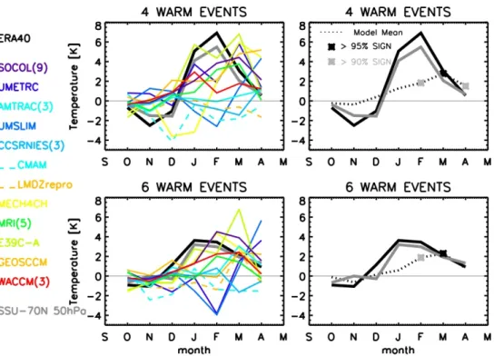
Because we are interested in changes that might be rel-evant for ozone, we summarize the reporting of the model response to ENSO by plotting the time evolution from Oc-tober to April of the zonal mean temperature response to ENSO in the lower stratosphere (30–70 hPa) over the po-lar cap (70◦N–90◦N) as shown in Fig. 2. The results from ERA40 and SSU shown in Fig. 2 reproduce those deduced from Fig. 1. In Fig. 2 (left), one curve per model is plotted, i.e. the anomaly has been averaged over the set of multiple realizations performed by the same model, when available, in order to reduce the number of lines in the plot. In the right panels of Fig. 2 we estimate the response to ENSO, by com-puting the mean of all simulations and its significance, the latter estimated with a t-Student test performed over the total number (30) of available simulations.
For the 4 WE anomaly (Fig. 2 top-right), the largest tem-perature warming is obtained in February (about 7 K for
29 Figure 1. Monthly zonal mean temperature ENSO anomalies (ENSO minus NEUTRAL composites) from October to April at 70°N in zonal mean temperature for (left) the MSU4/SSU satellite and (right) ERA40 reanalysis, considering (top) the 4 and (bottom) the 6 major events from 1980 to 1999. Horizontal bar reports grey shadings showing the significance levels. Contour interval: 2K, dotted lines represent negative values.
Fig. 1. Monthly zonal mean temperature ENSO anomalies (ENSO minus NEUTRAL composites) from October to April at 70◦N in zonal mean temperature for (left) the MSU4/SSU satellite and (right) ERA40 reanalysis, considering (top) the 4 and (bottom) the 6 major events from 1980 to 1999. Horizontal bar reports grey shadings showing the significance levels. Contour interval: 2 K, dotted lines represent negative values.
ERA40 and 5.5 K in SSU), whereas for the mean of all model simulations the largest warming is found in March (2.8 K, significant at 95%). The mean of all model simulations is positive and significant in February (2 K, significant at 90%) and in April (1.8 K, significant at 90%). The warming for the mean of all model simulations in late winter and spring is rel-atively small compared with the reanalysis and satellite data, because the models show quite variable responses (see the spread of the colored curves on Fig. 2, left). For some mod-els, the largest positive anomaly at these altitudes is found in January or even in March-April; for three of them the posi-tive anomaly is greater than SSU, but lower than ERA40; and three models do not show any warming in this layer. Bear-ing in mind the internal stratospheric variability, we can con-clude that the ERA40, SSU and the model results are consis-tent and agree within the uncertainties. Associated with this stratospheric warming, a weakening of the polar vortex is found, that is highly variable across the models (not shown). The zonal mean temperature response to ENSO in the tropi-cal lower stratosphere (not shown) reports a cooling of about
−1 K in February and −0.5 K in March for ERA40. About half of this cooling is reproduced by the mean of all model simulations.
The analysis of Figs. 1 and 2 shows that the time evo-lution of the temperature anomaly for the 6 warm ENSO events, with the two additional events not disturbed by the volcanic external forcing, is similar but slightly weaker than the anomaly for the 4 largest ENSO events for the model mean. From here on the analysis will focus on the 4 warm ENSO composite only.
4 Troposphere teleconnection and link to the response
in the stratosphere
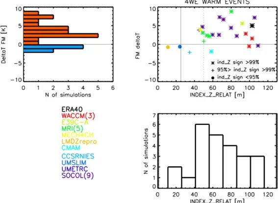
In order to relate the modeled response in the polar lower stratosphere to the representation of the ENSO teleconnec-tions within the troposphere (specifically, in the mid-latitude North Pacific region), the relationship between the 1Z in-dex (see Sect. 2), measure of the ENSO tropospheric tele-connection, and the 1T index, measure of February–March polar lower stratosphere temperature anomaly, is shown in Fig. 3 (the 1Z index has been calculated for 24 of the 30 simulations).
The 1T index distribution across the simulations tends to be positive (Fig. 3, top-left): 18 simulations show pos-itive response, 6 simulations a negative response, with the largest occurrence in the positive anomaly associated to the 2–3 K bin. These results summarize Fig. 2. The distribution
30 Figure 2. (Left) Monthly zonal mean temperature ENSO anomalies from October to April, averaged over the polar cap (70°N-90°N) and the (30-70 hPa) pressure band, for each model, ERA40 (black thick line) and SSU (grey thick line). SSU anomalies are calculated at 70°N and 50hPa. Concerning the simulations (colored lines), one curve per model is plotted, i.e. the anomaly has been averaged over the ensemble members, when available. (Right) the mean of all simulations calculated over the 30 models (dotted line) and, repeated from the left panel, ERA40 (black thick line) and SSU (grey thick line). Superimposed are significances at more than 90% (grey stars) and 95% (black stars) for the model mean. (Top) 4 ENSO events and (bottom) 6 ENSO events.
Fig. 2. (Left) Monthly zonal mean temperature ENSO anomalies from October to April, averaged over the polar cap (70◦N–90◦N) and the (30–70 hPa) pressure band, for each model, ERA40 (black thick line) and SSU (grey thick line). SSU anomalies are calculated at 70◦N and 50 hPa. Concerning the simulations (colored lines), one curve per model is plotted, i.e. the anomaly has been averaged over the ensemble members, when available. (Right) the mean of all simulations calculated over the 30 models (dotted line) and, repeated from the left panel, ERA40 (black thick line) and SSU (grey thick line). Superimposed are significances at more than 90% (grey stars) and 95% (black stars) for the model mean. (Top) 4 ENSO events and (bottom) 6 ENSO events.
of the 1Z index across the simulations (shown in Fig. 3 bottom-right) indicates that the response is variable also for this index. This index is a quantitative estimate of the tropospheric stationary wave anomaly during strong ENSO episodes. Consequently, a large value of this index can imply an increase of vertically propagating planetary waves emerg-ing from the troposphere (see the Appendix A for an exam-ple).
The maximum occurrence for this index for the model data pool is found in the 40–55 m bin whereas the 1Z index for ERA40 is larger (103 m). In Fig. 3 top-right are shown the 1-standard deviation and 2-standard deviations for the 1Z index of ERA40 (the vertical continuous and dotted lines, re-spectively); note that the maximum occurrence of the 1Z index for the model simulations is close to the 2-sigma value of ERA40. The 1Z index for ERA40 is about four times its standard deviation, whereas for the majority of the model simulations the ratio of this index with respect to its stan-dard deviation is smaller (about 3, not shown). This result shows that the ENSO tropospheric stationary wave anoma-lies are larger (and with higher variability) for ERA40 than for the majority of the simulations (note that ERA40 is dom-inated by the large 1998 ENSO event, not shown). This dis-cussion implies that the ENSO extratropical response in the
eddy geopotential height field is robust for ERA40. For the majority of the model simulations the tropospheric signal as-sociated to ENSO, even if smaller, is robust as well as the
1Z index is significant at 99% with respect to their stan-dard deviation (the simulations satisfying this are indicated by stars). Only two models (LMDZrepro and UMSLIMCAT) have a non-significant 1Z index (dots in Fig. 3 top-right), three models show a 1Z index with a significance ranging between 95% and 99% (indicated by crosses).
From the above analysis of the 1Z index it is implied that the model simulations that do not have a strong enough extra-tropical ENSO teleconnection pattern in the troposphere are not supposed to have a response in the stratosphere. Indeed, the two models that do not reproduce a significant tropo-spheric extratropical ENSO signal report a temperature re-sponse that is close to zero, or slightly negative (Fig. 3 top-right). The rest of the model simulations (the majority) are in good agreement with ERA40, in the sense that they are clustered in the region of positive 1T index and larger than 2-standard deviation ERA40 1Z index. Their positive tem-perature response in the stratosphere (evidenced also by the histogram) is however characterized by a large spread. This spread is therefore due to the modeled stratospheric internal variability.
31 Figure 3. (Top-left) Histogram of the temperature (K) anomaly of Figure 2 (4WE = 4 warm events), averaged over February and March (deltaT FM) for 24 models; red/blue bars indicate the number of model simulations with positive/negative temperature response. (Top-right) scatter plot for each model (listed in table 1) and ERA40 of the temperature (K) anomaly of Figure 2, averaged over February and March (ΔT index), versus the ΔZ index (m; index_z_relat) at 500 hPa;. (Bottom-right) histogram of the ΔZ index (m) at 500 hPa for the models. The simulations with a ΔZ index significant at 99% and 95% are represented by stars and crosses, respectively; the simulations with a non-significant ΔZ index are shown by dots. 1-standard deviation and 2-standard deviations for the ΔZ index of ERA40 are shown as the vertical continuous and dotted lines, respectively.
Fig. 3. (Top-left) Histogram of the temperature (K) anomaly of Fig. 2 (4 WE=4 warm events), averaged over February and March (1T FM) for 24 models; red/blue bars indicate the number of model simulations with positive/negative temperature response. (Top-right) scatter plot for each model (listed in Table 1) and ERA40 of the temperature (K) anomaly of Fig. 2, averaged over February and March (1T index), versus the 1Z index (m; index z relat) at 500 hPa; (Bottom-right) histogram of the 1Z index (m) at 500 hPa for the models. The simulations with a 1Z index significant at 99% and 95% are represented by stars and crosses, respectively; the simulations with a non-significant 1Z index are shown by dots. 1-standard deviation and 2-standard deviations for the 1Z index of ERA40 are shown as the vertical continuous and dotted lines, respectively.
Another important result of Fig. 3 is that differences among the simulations in the 1Z index are almost twice larger than the differences within the multiple realization runs of a model (see the 1Z index range for WACCM, MRI, and SOCOL). As discussed above, an explanation of this result is that the tropospheric ENSO teleconnection is sub-stantially different for some of the models. Although also the spread in this index among the model simulations with a significant 1Z index can be related to the variability of the ENSO extra-tropical tropospheric teleconnections, for the models with an insignificant index it should be mainly related to model formulation. On the other hand, the comparable spread (−2 K to 9 K) in the 1T index among all the model simulations is indicative of the modeled stratospheric internal variability, and suggests that even with a similar ENSO tele-connection in the troposphere (see for example WACCM), there is variability in the lower stratospheric temperature re-sponse.
5 Ozone
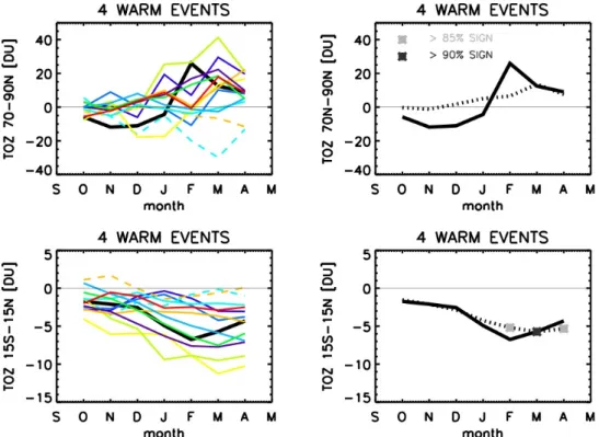
The impact of ENSO on the column ozone distribution is illustrated in Fig. 4 for the models, the NIWA dataset and for the mean of all model simulations, at polar latitudes (70◦N– 90◦N average, top) and in the Tropics (15◦S–15◦N average, bottom).
In the polar region, the NIWA column ozone anomaly is negative from October to January and positive in February, March and April. The NIWA total ozone positive anomaly is largest in February (∼20 DU). The model responses show a large spread, especially in January, February and March. The column ozone anomaly in the mean of all model simula-tions is positive from January to April and reaches ∼10 DU in March (not significant). In the tropical regions (Fig. 4, bottom), negative ozone anomalies are observed throughout the whole winter season. The largest negative anomalies are again obtained for the same months: in February (−7 DU) for NIWA and in March (−6 DU, significant at 95%) for the mean of all model simulations. Figure 4 demonstrates that an increase of the column ozone in the Arctic (top) is
32 Figure 4. Monthly zonal mean column ozone (DU) ENSO anomalies from October to April, averaged over the polar cap (70°N-90°N) (top-left) and between (15°N-15°S) (bottom-left), for each model and for NIWA (black curve). The color code for the models is the same as Figure 2. One curve per model is plotted, i.e. the anomaly has been averaged over the ensemble members, when available. (Right) the mean of all simulations (black dots) and NIWA (black curve). Superimposed are significances at more than 90% (grey stars) and 95% (black stars) for the mean of all simulations.
Fig. 4. Monthly zonal mean column ozone (DU) ENSO anomalies from October to April, averaged over the polar cap (70◦N–90◦N) (top-left) and between (15◦N–15◦S) (bottom-left), for each model and for NIWA (black curve). The color code for the models is the same as Fig. 2. One curve per model is plotted, i.e. the anomaly has been averaged over the ensemble members, when available. (Right) the mean of all simulations (black dots) and NIWA (black curve). Superimposed are significances at more than 90% (grey stars) and 95% (black stars) for the mean of all simulations.
Figure 5. Scatter plot of the ΔO3 index (column ozone ENSO anomaly, DU, of Figure 4 top-left averaged over February and March) versus the ΔT index (temperature anomaly, K, of Figure 2, averaged over February and March). Black star: the NIWA ΔO3 index (DU) versus the ERA40 ΔT index (K).
Fig. 5. Scatter plot of the 1O3 index (column ozone ENSO
anomaly, DU, of Fig. 4 top-left averaged over February and March) versus the 1T index (temperature anomaly, K, of Fig. 2, averaged over February and March). Black star: the NIWA 1O3index (DU)
versus the ERA40 1T index (K).
accompanied by a coherent column ozone decrease at tropi-cal latitudes (bottom).
The accumulation of ozone at high latitudes is indicative of stronger diabatic descent during ENSO in that region, consistent with a warmer polar lower stratosphere (Fig. 2) and an increased Brewer Dobson circulation. The column ozone decrease in the tropics is consistent with increased ascent in the lower stratosphere circulation and, again, in-creased Brewer-Dobson circulation. As for the temperature, the column ozone anomaly across the models at high lati-tudes is highly variable showing a large spread in the model responses. In the tropics, the response across the models is consistent and quite robust (Fig. 4, bottom-left and the signif-icance in the bottom-right). Note however that in the tropics the column ozone is also directly affected by ENSO, because during ENSO the warmer sea surface temperatures lead to a warmer troposphere and a higher tropopause throughout most of the tropics. The higher tropopause in turn implies a decrease of the tropical column ozone (Shiotani, 1992; Stein-brecth et al., 2006). The response in the tropical lower strato-sphere can also be directly related to local tropical wave forc-ing (Deckert and Dameris, 2008) a topic not addressed in the current work.
34 Figure 6. (Left) Histogram of the ΔO3(FM-ND) index (the column ozone anomaly, DU, average of February and March, minus the November - December average) for all the models at 60°N-90°N (top) and 15°N-15°S (bottom); red/blue bars indicate the number of model simulations with positive/negative temperature response. (Right) scatter plot of the ΔO3(FM-ND) index versus the ΔZ index (m) at 60°N-90°N (top) and 15°N-15°S (bottom) for all models (in color, coded as in Figure 3). Black stars represent the NIWA ΔO3(FM-ND) index versus the ERA40 ΔZ index. The simulations with a ΔZ index significant at 99% and 95% are represented by stars and crosses, respectively; the simulations with a non-significant ΔZ index are shown by dots. 1-standard deviation and 2-standard deviations for the ΔZ index of ERA40 are shown as the vertical continuous and dotted lines, respectively.
Fig. 6. (Left) Histogram of the 1O3(FM-ND) index (the column ozone anomaly, DU, average of February and March, minus the November–
December average) for all the models at 70◦N–90◦N (top) and 15◦N–15◦S (bottom); red/blue bars indicate the number of model simulations with positive/negative temperature response. (Right) scatter plot of the 1O3(FM-ND) index versus the 1Z index (m) at 70◦N–90◦N (top)
and 15◦N–15◦S (bottom) for all models (in color, coded as in Fig. 3). Black stars represent the NIWA 1O3(FM-ND) index versus the ERA40 1Z index. The simulations with a 1Z index significant at 99% and 95% are represented by stars and crosses, respectively; the simulations with a non-significant 1Z index are shown by dots. 1-standard deviation and 2-standard deviations for the 1Z index of ERA40 are shown as the vertical continuous and dotted lines, respectively.
Figure 5 reports a scatter plot of the 1O3index versus the 1T index. This figure shows that the ENSO response in 1O3
and 1T for the majority of the models is located in the upper-right quadrant, in agreement with the signature from observa-tions. Moreover, a clear positive correlation (0.85, significant at more than 99.9%) between the modeled column ozone and temperature anomalies is found. This relationship is con-sistent with the one expected from inter-annual variability. Indeed, the slope deduced from Fig. 5 (about 5 DU/K) is close to the slope calculated using the ERA40 temperature and NIWA column ozone from the pool of all the individual years (about 5.5 DU/K; not shown). Moreover, Fig. 5 shows that the positive correlation appears also for the 9 realiza-tions from the SOCOL model and possibly the 5 realizarealiza-tions from the MRI model, and that the spread among the models is comparable to the spread among the same-model realiza-tions of either SOCOL or MRI. These results indicate that the cause of the spread in the modeled responses is physical (as opposed to be due to unphysical biases in the models), and it is due to modeled internal variability. The internal strato-spheric variability appears to play a dominant role, possibly obscuring differences due to model formulation.
The anomalous wintertime increase of column ozone at high latitudes and decrease at low latitudes is defined as the anomalous tendency of column ozone from the beginning of winter to the end of winter/beginning of spring and is ana-lyzed following Salby and Callaghan (2002) and Fusco and Salby (1999). Figure 6 (left) shows the distribution of the
1O3(FM-ND) index (Sect. 2) at polar (top) and tropical
(bot-tom) latitudes. The distribution of the 1O3(FM-ND) index
is clearly negative at tropical latitudes (with 23 simulations reporting a negative index and just one realization with a pos-itive index) whilst it is generally pospos-itive (17 models) at high latitudes. In this case, the anomalous wintertime increase of column ozone at high latitudes represents the column ozone dynamical accumulation (i.e. ozone that is transported by anomalous residual circulation) with a negligible contribu-tion of the dynamically-induced chemical effect (i.e. changes in ozone due to changes in photochemistry induced by dy-namical changes in temperature), because ENSO years are anomalously warm.
In order to quantify the sensitivity of the anomalous strato-spheric ozone accumulation controlled by dynamical vari-ability to the tropospheric forcing in the North Pacific region
during ENSO, Fig. 6 (right) shows the scatter plot of the win-tertime dynamical ozone accumulation during ENSO (the
1O3(FM-ND) index) together with the 1Z index, as
al-ready done for the anomalous temperature in Fig. 3. Fig-ure 6 shows that model simulations that are in good agree-ment with ERA40 (modeled 1Z index larger than 2-standard deviations ERA40 1Z index) simulate a dynamically accu-mulated ozone during ENSO at polar latitudes and a decrease at low latitudes, reflecting enhanced stratospheric transport, as expected from previous analysis of Figs. 3 and 5. In partic-ular, as in Fig. 3, the only two models with a non-significant (at 95%) 1Z index (dots in Fig. 6) report a response in ozone at both latitudinal bands that is close to zero (as for tempera-tures in Fig. 3).
The ozone sensitivity to the strength of the ENSO forc-ing into the troposphere deduced from Fig. 6 shows that an increasing of the tropospheric forcing in the North Pacific region during ENSO of about 2–3 standard deviations im-plies a modeled wintertime ozone accumulation of about 15– 25 DU (and a simultaneous reduction ranging between −2 and −5 DU in the Tropics). These quantities for the obser-vational datasets are ∼30 DU in the Arctic (−5 DU in the Tropics), with an enhanced tropospheric ENSO forcing of about 4 standard deviations. Therefore, the modeled ozone sensitivity to the strength of the tropospheric ENSO forcing is in good agreement with the observational datasets.
6 Summary and conclusions
A systematic CCM inter-comparison of the stratospheric temperature and ozone response to ENSO for the Northern winter is reported. The model simulations considered here are those used for the CCMVal-1 activity (presented and dis-cussed in Eyring et al., 2006), of which many contributed to the last ozone assessment (WMO/UNEP, 2007). The main results are summarized here:
1. In the lower stratosphere, the mean of all model sim-ulations reports a warming of the polar vortex during strong ENSO events: The February-March temperature anomaly in the lower stratosphere is positive, signifi-cant and of the order of 2 K for the mean of all model simulations. The response to ENSO obtained from the individual simulations is however highly variable, be-cause of the large internal atmospheric variability and possibly also because of differences in model formula-tions. The mean anomaly derived from the model simu-lations is consistent with but smaller (∼2 K) than the estimate from the SSU temperature (∼4 K) and from ERA40 (∼6 K) in the lower stratosphere.
2. The warming found in the mean of all model simula-tions in the polar lower stratosphere is associated with an increase of column ozone north of 70◦N: The col-umn ozone ENSO anomaly in the mean of all model
simulations is positive and of the order of 10 DU in March. The dynamical increase of the column ozone in the Arctic during ENSO is accompanied by coherent column ozone decrease in the Tropics (7 DU). The mod-eled anomalies are in very good agreement with those derived by the NIWA column ozone in the Tropics and consistent but about one half of the anomalies found with NIWA in the Arctic (∼20 DU in February). 3. The 1Z index represents a measure of the eastward
elongation of the north-west Pacific trough during warm ENSO years. As discussed in Manzini et al. (2006), this structure is persistent in time and may enhance the tropospheric forcing of upward propagating planetary wave one (see also the Appendix A). Once the plane-tary wave one is enhanced also in the stratosphere, it can affect the zonal mean flow (by wave-mean flow interac-tion) and give rise to large-scale effects. The analysis of the 1Z index reveals that the temperature and ozone response in the lower stratosphere depend on the repre-sentation of the tropospheric ENSO teleconnection: For the most of the model simulations that have a significant ENSO teleconnection pattern in the troposphere, the Arctic lower stratosphere is warmer, and the response in ozone is characterized by, an increased ozone dynami-cal accumulation in the polar latitudes and a decrease at tropical latitudes, consistent with increased circula-tion in the stratosphere. Conversely, the model simu-lations that do not have a strong enough extra-tropical ENSO teleconnection pattern in the troposphere (and that therefore are not supposed to have a response in the stratosphere) show indeed a stratospheric signal close to zero.
4. Even if the modeled ozone anomalies are smaller that the anomalies found with NIWA in the Arctic, the mod-eled ozone sensitivity to the strength of the tropospheric ENSO forcing is in good agreement with the observa-tional datasets: from about 15 to 25 DU in the Arctic (from −2 to −5 DU in the Tropics) for an increase of the ENSO forcing of about 2–3 standard deviations in the models; ∼30 DU in the Arctic (−5 DU in the Trop-ics) for an increase of about 4 standard deviations in the observations.
5. The role of modeled internal variability in the polar stratospheric ENSO response has been deduced by the spread in the temperature and ozone ENSO anomalies for the models that provided more than one realization of the 20-year period considered. We have found that the spread of the 1Z index among the models tends to be larger than the spread within the realizations ob-tained by one model (MRI, SOCOL, WACCM). In par-ticular, for the SOCOL model, for which there are 9 re-alizations, the spread between its realizations is about half the total spread. We also notice that only two
models (LMDZrepro and UMSLIMCAT) report a 1Z index that is non-significant and is below one standard deviation (∼25 m) of the stationary eddies of ERA40, suggesting that the tropospheric ENSO teleconnection for these models is underestimated, because of model biases in the representation of tropospheric processes. These results imply that tropospheric variability and dif-ferences in representing ENSO teleconnection in the troposphere, due to differences in model formulations, play a substantial role in the stratospheric response to ENSO.
To summarize, our systematic intercomparison of the sensitivity of the response to ENSO in the stratosphere for CCMs included in the CCMVal-1 activity is in agree-ment with previous analysis based on observational datasets (Br¨onnimann, 2004), the SOCOL CCM (e.g. Fischer et al., 2008; Br¨onnimann et al., 2006) and other modeling studies (e. g. Sassi et al., 2004; Manzini et al., 2006). Namely, also the mean of all simulations from the pool of models con-sidered here display a polar warming and increased column ozone during ENSO years. Differently from the mentioned works in this analysis the ENSO signal in the lower strato-sphere is considered to be non linear, through the use of the composite technique (following Manzini et al., 2006 and Ho-erling 1997).
The reported modeled and observed warming in FM lower stratosphere and increase (decrease) in total column ozone at high (low) latitudes, is consistent with increased residual circulation during ENSO. Given the spread in the tempera-ture and the ozone responses to ENSO, within the pool of available simulations, the strength of this increase is presum-ably also highly variable. The positive correlation (signif-icant at more than 99%) and the slope found between the ENSO anomaly in temperature and column ozone indicates that interannual variability is the main driver for the 1T ,
1O3covariance, hence interannual variability explains the
spread in response to ENSO.
The responses in the lower stratospheric temperature and in column ozone are highly variable indicating that the large internal stratospheric variability in the models plays a major role in determining these responses. Nevertheless, by quan-tifying the tropospheric stationary eddy enhancement during ENSO and its variability across the model simulations, we have shown that the tropospheric ENSO teleconnections are important in explaining the range of responses in the lower stratospheric temperature and in column ozone. In fact, our analysis suggests a strong link between the dynamical ENSO external forcing of the stratosphere and the strength of the response in the stratosphere. This result is therefore the most promising for being used to differentiate between the role of internal variability and model formulation in a larger pool of realizations and models and it highlights that tropo-spheric modeling (specifically the parameterizations of the processes related to diabatic heating and the modeled mean
36 Figure A. Scatter plot of (top) the February-March temperature at 50 hPa averaged between 70°-90°Nand the January-February eddy heat flux anomalies at 100 hPa averaged between 45°N-75°N; (bottom) the January-February heat flux anomaly at 100 hPa averaged between 45°N-75°N and the new ΔZ* index. Grey stars represent the ENSO years. Data from one simulation of the MRI model.
Fig. A1. Scatter plot of (top) the February–March temperature at 50 hPa averaged between 70◦–90◦N and the January–February eddy heat flux anomalies at 100 hPa averaged between 45◦N– 75◦N; (bottom) the January–February heat flux anomaly at 100 hPa averaged between 45◦N–75◦N and the new 1Z∗index. Grey stars represent the ENSO years. Data from one simulation of the MRI model.
state) is important when attempting to accurately simulate the stratospheric response to ENSO forcing in Chemistry Cli-mate Models.
Appendix A
The link between the 1Z index, defined in Sect. 2.3 and dis-cussed in Sect. 4, and the eddy heat flux at 100 hPa is detailed here.
Figure A1 shows (top) the correlation between the February-March polar cap averaged temperature at 50 hPa and the January–February heat flux anomaly at 100 hPa av-eraged between 45◦–75◦N, for each single year of one of the MRI simulations (as an example); and (bottom) the cor-relation between the January–February heat flux anomaly at 100 hPa averaged between 45◦–75◦N and a new 1Z∗index calculated in the following way: at 500 hPa, 50◦N and for the 1Z index longitude, for each year of the 1980–1999 period, the difference between the DJF averaged stationary eddy geopotential height of that year and its climatology as computed from the NEUTRAL years (NEUTRAL years
defined in Table 2). This computation implies that the aver-age of 1Z∗for the 4 warm ENSO years is the 1Z index used in Fig. 3. In grey are the signatures for the 4 ENSO events used in Fig. 3 and the two additional ones used in Fig. 2. Fig-ure A1 (top) shows that three events (1983, 1992, 1998) of the four strongest events lie at the up-right side of this scatter plot: For three of the four largest ENSO events, the tempera-ture and heat flux are grouped together as the strongest ones. Figure A1 (top) therefore supports the notion that that the heat flux is high for warm ENSO. Figure A1 (bottom) shows that there actually appears to be also a linear relationship be-tween the January-February heat flux anomalies at 100 hPa and the 1Z∗index for the MRI simulation, and that it is in agreement with our expectation: ENSO years are character-ized by large heat fluxes and 1Z∗indices (grey signatures).
Acknowledgements. Chiara Cagnazzo is supported by the Centro
Euro-Mediterraneo per i Cambiamenti Climatici. Elisa Manzini acknowledges the support of the EC SCOUT-O3 Integrated Project (505390-GOCE-CT-2004) for part of this work. Natalia Calvo was supported by the Spanish Ministry of Education and Science and the Fulbright Commission in Spain. CCSRNIES’s research has been supported by the Global Environmental Research Fund (GERF) of the Ministry of the Environment (MOE) of Japan (A-071). MRI simulations have been made partly with the MRI supercomputer and partly with the NIES supercomputer. CMAM simulations were supported by the Canadian Foundation for Climate and Atmospheric Sciences and run on the Environment Canada Supercomputer. We acknowledge the modeling groups for making their simulations available for this analysis, the Chemistry-Climate Model Validation Activity (CCMVal) for WCRP’s (World Climate Research Programme) SPARC (Stratospheric Processes and their Role in Climate) project for organizing and coordinating the model data analysis activity, and the British Atmospheric Data Center (BADC) for collecting and archiving the CCMVal model output. Chiara Cagnazzo and Elisa Manzini are grateful to Antonio Navarra for useful discussions. We are thankful to John Austin for suggestions and discussions on the manuscript.
Edited by: W. Lahoz
References
Akiyoshi, H., Zhou, L. B., Yamashita, Y., Sakamoto, K., Yoshiki, M., Nagashima, T., Takahashi, M., Kurokawa, J., Takigawa, M., and Imamura, T.: A CCM simulation of the breakup of the Antarctic polar vortex in the years 1980–2004 un-der the CCMVal scenarios, J. Geophys. Res., 114, D03103, doi:10.1029/2007JD009261, 2009.
Akiyoshi, H., Sugita, T., Kanzawa, H., and Kawamoto, N.: Ozone perturbations in the Arctic summer lower stratosphere as a re-flection of NOx chemistry and planetary scale wave activity, J. Geophys. Res., 109, D03304, doi:10.1029/2003JD003632, 2004. Austin, J.: A three-dimensional coupled chemistry-climate model simulation of past stratospheric trends, J. Atmos. Sci., 59, 218– 232, 2002.
Austin, J. and Butchart, N.: Coupled chemistry-climate model sim-ulation for the period 1980 to 2020: Ozone depletion and the
start of ozone recovery, Q. J. Roy. Meteorol. Soc., 129, 3225– 3249, 2003.
Austin, J. and Wilson, R. J.: Ensemble simulations of the de-cline and recovery of stratospheric ozone, J. Geophys. Res., 111, D16314, doi:10.1029/2005JD006907, 2006.
Austin, J., Wilson, R. J., Li, F., and Voemel, H.: Evolution of wa-ter vapor concentrations and stratospheric age of air in coupled chemistry- climate model simulations, J. Atmos. Sci., 64, 905– 921, 2007.
Beagley, S. R., de Grandpre’, J., Koshyk, J. N., McFarlane, N. A., and Shepherd, T. G.: Radiative-dynamical climatology of the first-generation Canadian Middle Atmosphere Model, Atmos. Ocean, 35, 293–331, 1997.
Bloom., S., da Silva, A., Dee, D., Bosilovich, M., Chern, J.-D., Pawson, S., Schubert, S., Sienkiewicz, M., Stajner, I., Tan, W.-W. and Wu, M.-L.: Documentation and validation of the God-dard Earth Observing System (GEOS) data assimilation system – Version 4, in Global Modeling Data Assimilation 104606, Tech. Rep. Ser. 26, NASA Goddard Space Flight Cent., Md., 2005. Bodeker, G. E., Shiona, H., and Eskes, H.: Indicators of Antarctic
ozone depletion, Atmos. Chem. Phys., 5, 2603–2615, 2005, http://www.atmos-chem-phys.net/5/2603/2005/.
Brindley, H. E., Geer, A. J., and Harries, J. E.: Climate variability and trend in SSU radiances: a comparison of model predictions and satellite observations in the middle stratosphere, J. Climate, 12, 3197–321, 1999.
Br¨onnimann, S., Luterbacher, J., Staehelin, J., Svendby, T. M., Hansen, G., and Svenøe, T.: Extreme climate of the global tro-posphere and stratosphere 1940–1942 related to El Nino, Nature, 431, 971–974, 2004.
Br¨onnimann, S., Schraner, M., M¨uller, B., Fischer, A., Brunner, D., Rozanov, E., and Egorova, T.: The 1986–1989 ENSO cycle in a chemical climate model, Atmos. Chem. Phys., 6, 4669–4685, 2006,
http://www.atmos-chem-phys.net/6/4669/2006/.
Cagnazzo, C. and Manzini, E.: Impact of the stratosphere on the winter tropospheric teleconnections between ENSO and the North Atlantic and European Region, J. Climate, 22(5), 1223– 1238, 2009.
Camp, C. D. and Tung, K.-K.: Stratospheric polar warming by ENSO in winter: A statistical study, Geophys. Res. Lett., 34, L04809, doi:10.1029/2006GL028521, 2007.
de Grandpre, J., Beagley, S. R. , Fomichev, V. I., Griffioen, E., Mc-Connell, J. C., Medvedev, A. S., and Shepherd, T. G.: Ozone climatology using interactive chemistry: Results from the Cana-dian Middle Atmosphere Model, J. Geophys. Res., 105, 26475– 26492, 2000.
Deckert, R. and Dameris, M.: Higher tropical SSTs strengthen the tropical upwelling via deep convection, Geophys. Res. Lett., 35, L10813, doi:10.1029/2008GL033719, 2008.
Egorova, T., Rozanov, E., Zubov, V., Manzini, E., Schmutz, W., and Peter, T.: Chemistry-climate model SOCOL: A validation of the present-day climatology, Atmos. Chem. Phys., 5, 1557–1576, 2005,
http://www.atmos-chem-phys.net/5/1557/2005/.
Eyring, V., Butchart, N., Waugh, D., et al.: Assessment of tem-perature, trace species, and ozone in chemistry-climate model simulations of the recent past, J. Geophys. Res., 111, D22308, doi:10.1029/2006JD007327, 2006.
Fioletov, V. E. and Shepherd, T. G.: Seasonal persistence of mid-latitude total ozone anomalies, Geophys. Res. Lett., 30, 1417, doi:10.1029/2002GL016739, 2003.
Fischer, A. M., Shindell, D. T., Winter, B., Bourqui, M. S., Faluvegi, G., Rozanov, E., Schraner, M., and Br¨onnimann, S.: Stratospheric winter climate response to ENSO in three chemistry-climate models, Geophys. Res. Lett., 35, L13819, doi:10.1029/2008GL034289, 2008.
Free, M., and Seidel, D. J.: The observed ENSO tem-perature signal in the stratosphere, J. Geophys. Res., doi:10.1029/2009JD012420, in press, 2009.
Fusco, A. C. and Salby, M. L.: Interannual variations of total ozone and their relationship to variations of planetary wave activity, J. Climate, 12, 1619–1629, 1999.
Garcia, R. R., Marsh, D. R., Kinnison, D. E., Boville, B. A., and Sassi, F.: Simulation of secular trends in the mid-dle atmosphere, 1950–2003, J. Geophys. Res., 112, D09301, doi:10.1029/2006JD007485, 2007.
Garcia-Herrera, R., Calvo, N., Garcia, R. R., and Giorgetta, M. A.: Propagation of ENSO temperature signals into the middle atmosphere: A comparison of two general circulation models and ERA-40 reanalysis data, J. Geophys. Res., 111, D06101 doi:10.1029/2005JD006061, 2006.
Garfinkel, C. I. and Hartmann, D. L.: Effects of El Nino – South-ern Oscillation and the Quasi-Biennial Oscillation on polar tem-peratures in the stratosphere, J. Geophys. Res., 112, D19112, doi:10.1029/2007JD008481, 2007.
Garny, H., Dameris, M., and Stenke, A.: Impact of prescribed SSTs on climatologies and long-term trends in CCM simulations, At-mos. Chem. Phys., 9, 6017–6031, 2009,
http://www.atmos-chem-phys.net/9/6017/2009/.
Hadjinicolaou, P., Pyle J. A., Chipperfeld, M. P., and Kettleborough, J. A.: Effect of interannual meteorological variability on middle latitude O3, Geophys. Res. Lett., 24, 2993–2996, 1997.
Hamilton, K.: An examination of observed Southern Oscillation effects in the Northern Hemisphere stratosphere, J. Atmos. Sci., 50, 3468–3473, 1993.
Hoerling, M. P., Kumar, A., and Zhong, M.: El Ni˜no, La Ni˜na, and the nonlinearity of their teleconnections, J. Climate, 10, 1769– 1786, 1997.
Kurokawa, J., Akiyoshi, H., Nagashima, T., Masunaga, H., Nakajima, T., Takahashi, M., and Nakane, H.: Effects of atmospheric sphericity on stratospheric chemistry and dy-namics over Antarctica, J. Geophys. Res., 110, D21305, doi:10.1029/2005JD005798, 2005.
Kuroda, Y. and Kodera, K.: Variability of the polar-night jet in the northern and southern hemispheres, J. Geophys. Res., 106(D18), 20703–20713, 2001.
Labitzke, K. and van Loon, H.: The Southern Oscillation. Part IX: The influence of volcanic eruptions on the Southern Oscillation in the stratosphere, J. Climate, 2, 1223–1226, 1989.
Lefevre, F., Brasseur, G. P., Folkins, I., Smith, A. K., and Simon, P.: Chemistry of the 1991–1992 stratospheric winter: Three di-mensional model simulations, J. Geophys. Res., 99, 8183–8195, 1994.
Manzini, E., Steil, B., Br¨uhl, C., Giorgetta, M. A., and Kr¨uger, K.: A new interactive chemistry-climate model: 2. Sensitivity of the middle atmosphere to ozone depletion and increase in green-house gases and implications for recent stratospheric cooling,
J. Geophys. Res., 108(D14), 4429, doi:10.1029/2002JD002977, 2003.
Manzini, E., Giorgetta, M. A., Esch, M., Kornblueh, L., and Roeckner, E.: The influence of sea surface temperatures on the northern winter stratosphere: Ensemble simulations with the MAECHAM5 model, J. Climate, 19, 3863–3881, 2006. Nash, J. and Edge, P. R.: Temperature changes in the stratosphere
and lower mesosphere 1979–1988 inferred from TOVS radiance observations, Adv. Space Res., 9, 333–341, 1989.
Newman, P. A., Nash, E. R., and Rosenfield, J. E.: What controls the temperature of the Arctic stratosphere during the spring?, J. Geophys. Res., 106, 19999–20010, 2001.
Randel, W. J., Wu, F., and Stolarski, R.: Changes in column ozone correlated with the stratospheric EP fux, J. Meteorol. Soc. Japan, 80, 849–862, 2002.
Randel, W. J., Garcia, R. R., Calvo, N., and Marsh, D.: ENSO influence on zonal mean temperature and ozone in the trop-ical lower stratosphere, Geophys. Res. Lett., 36, L15822, doi:10.1029/2009GL039343, 2009.
Rozanov, E., Schraner, M., Schnadt, C., Egorova, T., Wild, M., Ohmura, A., Zubov, V., Schmutz, W., and Peter, T.: Assessment of the ozone and temperature variability during 1979–1993 with the chemistry-climate model SOCOL, Adv. Space Res., 35(8), 1375–1384, 2005.
Salby, M. L. and Callaghan, P. F.: Interannual Changes of the Stratospheric Circulation: Relationship to Ozone and Tropo-spheric Structure, J. Climate, 3673–3685, 2002.
Sassi, F., Kinnison, D., Boville, B. A., Garcia, R. R., and Roble. R.: Effect of El Ni˜no–Southern Oscillation on the dynamical, ther-mal, and chemical structure of the middle atmosphere, J. Geo-phys. Res., 109, D17108, doi:10.1029/2003JD004434, 2004. Scinocca, J. F., McFarlane, N. A., Lazare, M., Li, J., and Plummer,
D.: Technical Note: The CCCma third generation AGCM and its extension into the middle atmosphere, Atmos. Chem. Phys., 8, 7055–7074, 2008
Shibata, K. and Deushi, M.: Long-term variations and trends in the simulation of the middle atmosphere 1980–2004 by the chemistry-climate model of the Meteorological Research Insti-tute, Ann. Geophys., 26, 1299–1326, 2008a,
http://www.ann-geophys.net/26/1299/2008/.
Shibata, K. and Deushi, M.: Simulation of the stratospheric cir-culation and ozone during the recent past (1980–2004) with the MRI chemistry-climate model, CGER’s Supercomputer Mono-graph Report Vol. 13, National Institute for Environmental Stud-ies, Japan, 154 pp., 2008b.
Shiotani, M.: Annual, quasi-biennial, and E1 Nino-Southern Oscil-lation (ENSO) timescale variations in equatorial total ozone, J. Geophys. Res., 97, 7625–7633, 1992.
Spencer, R. W. and Christy, J. R.: Precision Lower Stratospheric Temperature Monitoring with the MSU: Technique, Validation, and Results 1979–1991, J. Climate, 6, 1194–1204, 1993. Steil, B., Bruehl, C., Manzini, E., Crutzen, P. J., Lelieveld, J.,
Rasch, P. J., Roeckner, E., and Krueger, K.: A new interactive chemistry-climate model: 1. Present-day climatology and inter-annual variability of the middle atmosphere using the model and 9 years of HALOE/UARS data, J. Geophys. Res., 108(D9), 4290, doi:10.1029/2002JD002971, 2003.
Steinbrecht, W., Hassler, B., Br¨uhl, C., Dameris, M., Giorgetta, M. A., Grewe, V., Manzini, E., Matthes, S., Schnadt, C., Steil,
B., and Winkler, P.: Interannual variation patterns of total ozone and temperature in observations and model simulations, Atmos. Chem. Phys., 6, 349–374, 2006,
http://www.atmos-chem-phys.net/6/349/2006/.
Stenke, A., Dameris, M., Grewe, V., and Garny, H.: Implications of Lagrangian transport for simulations with a coupled chemistry-climate model, Atmos. Chem. Phys., 9, 5489–5504, 2009, http://www.atmos-chem-phys.net/9/5489/2009/.
Stolarski, R. S., Douglass, A. R., Steenrod, S. and Pawson, S.: Trends in stratospheric ozone: Lessons learned from a 3d chem-ical transport model, J. Atmos. Sci., 63, 1028–1041, 2006. Strauss, D. M. and Shukla, J.: Distinguishing between the
SST-forced and internal variability in mid latitudes: Analysis of ob-servations and GCM simulations, Q. J. Roy. Meteor. Soc., 126, 2323–2350, 2000.
Struthers, H., Austin, J., Kreher, K., Bodeker, G., Schofield, R., Johnston, P., Shiona, H., and Thomas, A.: Past and future simu-lations of NO2from a coupled chemistry-climate model in
com-parison with observations, Atmos. Chem. Phys., 4, 2227–2239, 2004,
http://www.atmos-chem-phys.net/4/2227/2004/.
Tian, W. and Chipperfield, M. P.: A new coupled chemistry – cli-mate model for the stratosphere: The importance of coupling for future O3 – climate predictions, Q. J. Roy. Meteor. Soc., 131,
281–304, 2005.
Taguchi, M. and Hartmann, D. L.: Increased occurrence of stratospheric sudden warmings during El Nino as simulated by WACCM, J. Climate, 19(3), 324–332, 2006.
Uppala, S., Kallberg, P. W., Simmons, A. J., et al.: ERA-40: ECMWF 45-year reanalysis of the global atmosphere and surface conditions 1957–2002: ECMWF Newsletter, Vol. 101, ECMWF, Reading, United Kingdom, 2–21, 2004.
Uppala, S., Kallberg, P. , Hernandez, A., et al.: The ERA-40 re-analysis, Q. J. Roy. Meteor. Soc., 131, 2961–3211, 2005. Van Loon, H. and Labitzke, K.: The Southern Oscillation. Part V:
The anomalies in the lower stratosphere of the Northern Hemi-sphere in winter and a comparison with the quasi-biennial oscil-lation, Mon. Weather Rev., 115, 357–369, 1987.
Weber, M., Dhomse, S., Wittrock, F., Richter, A., Sinnhuber, B.-M., and Burrows, J. P.: Dynamical control of NH and SH win-ter/spring total ozone from GOME observations in 1995–2002, Geophys. Res. Lett., 30(11), 1583, doi:10.1029/2002GL016799, 2003.
World Meteorological Organization/United Nations Environment Programme (WMO/UNEP), Scientific Assessment of Ozone De-pletion: 2006, Rep. 50, World Meteorol. Org., Global Ozone Res. and Monit. Proj., Geneva, Switzerland, 2007.