Downscaled Rainfall Prediction Model (DRPM) using a Unit Disaggregation Curve (UDC)

(1)

HAL Id: hal-00298635

https://hal.archives-ouvertes.fr/hal-00298635

Submitted on 14 Apr 2005

HAL is a multi-disciplinary open access

archive for the deposit and dissemination of sci-entific research documents, whether they are pub-lished or not. The documents may come from teaching and research institutions in France or abroad, or from public or private research centers.

L’archive ouverte pluridisciplinaire HAL, est destinée au dépôt et à la diffusion de documents scientifiques de niveau recherche, publiés ou non, émanant des établissements d’enseignement et de recherche français ou étrangers, des laboratoires publics ou privés.

Downscaled Rainfall Prediction Model (DRPM) using a

Unit Disaggregation Curve (UDC)

S. Tantanee, S. Patamatamakul, T. Oki, V. Sriboonlue, T. Prempree

To cite this version:

S. Tantanee, S. Patamatamakul, T. Oki, V. Sriboonlue, T. Prempree. Downscaled Rainfall Prediction Model (DRPM) using a Unit Disaggregation Curve (UDC). Hydrology and Earth System Sciences Discussions, European Geosciences Union, 2005, 2 (2), pp.543-568. �hal-00298635�

(2)

HESSD

2, 543–568, 2005 DRPM using a UDC S. Tantanee et al. Title Page Abstract Introduction Conclusions References Tables Figures J I J I Back Close

Full Screen / Esc

Print Version Interactive Discussion

EGU

Hydrol. Earth Sys. Sci. Discuss., 2, 543–568, 2005 www.copernicus.org/EGU/hess/hessd/2/543/ SRef-ID: 1812-2116/hessd/2005-2-543 European Geosciences Union

Hydrology and Earth System Sciences Discussions

Downscaled Rainfall Prediction Model

(DRPM) using a Unit Disaggregation

Curve (UDC)

S. Tantanee1, S. Patamatamakul2, T. Oki3, V. Sriboonlue2, and T. Prempree2

1

Graduate School, Khon Kaen University, Muang, Khonkaen, Thailand

2

Engineering Faculty, Khon Kaen University, Muang, Khonkaen, Thailand

3

Institute of Industrial Science, University of Tokyo, Tokyo, Japan

Received: 9 March 2005 – Accepted: 22 March 2005 – Published: 14 April 2005 Correspondence to: S. Tantanee (stantanee@yahoo.com)

(3)

HESSD

Full Screen / Esc

EGU

Abstract

This study was undertaken to identify the process for generating finer time scaled rain-fall from higher time scaled data. The Downscaled Rainrain-fall Prediction Model (DRPM) using the technique of unit disaggregation curve (UDC) was developed under the con-cept of coupling the stochastic autoregressive (AR) model with a wavelet filter and

5

disaggregation model. Sequences of the number of rainy days and monthly rainfall were simulated from 52-year rainfall records at 4 stations in the northeastern part of Thailand. Compared with actual rainfall sequences, the 30 year generated sequences provided R-square values of 0.47–0.60. The model was applied to forecast the num-ber of rainy days and monthly rainfall for the year of 2002. When compared with actual

10

records the prediction model provided R-square values of 0.50 to 0.79.

1. Introduction

Various hydrological models need the predicted rainfall series to simulate the water resources system for future planning. Rainfall series are the hydrological time series composed of deterministic and stochastic components. In order to consider the

deter-15

ministic part, the nuances of the series, which is noise of signal, have to be eliminated. The deterministic part can describe the mathematical characteristics of the series. The dependency of stochastic components of the series can be analyzed using the au-toregressive (AR) model which is the model applied for analyzing the rainfall series (Thomas and Fiering, 1962; Yevjevich, 1963; Box and Jenkins, 1970). Normally, the

20

hydrological process is studied in different time scales. Several disaggregation models have been developed for numerous hydrological applications (Valencia and Shaake, 1973; Mejia and Rousselle, 1976; Hoshi and Burgs, 1979; Stedinger and Vogel, 1984; Koutsoyiannis, 1992). In recent years, the wavelet transform has been successfully applied to wave data analysis and other ocean engineering applications (e.g. Lau and

25

Weng, 1995; Massel, 2001; Teisseire et al., 2002; Huang, 2004). The objective of this 544

(4)

HESSD

Full Screen / Esc

EGU

study is to develop the process for rainfall prediction by coupling a wavelet filter with AR and the disaggregation concept. The unit disaggregation curve (UDC) technique was also developed in order to describe the pattern of rainfall distribution within a year. The proposed model is the downscaled prediction model of annual to monthly series, which is the time scale required in the simulation model for the purpose of water resources

5

planning and management.

2. Data input

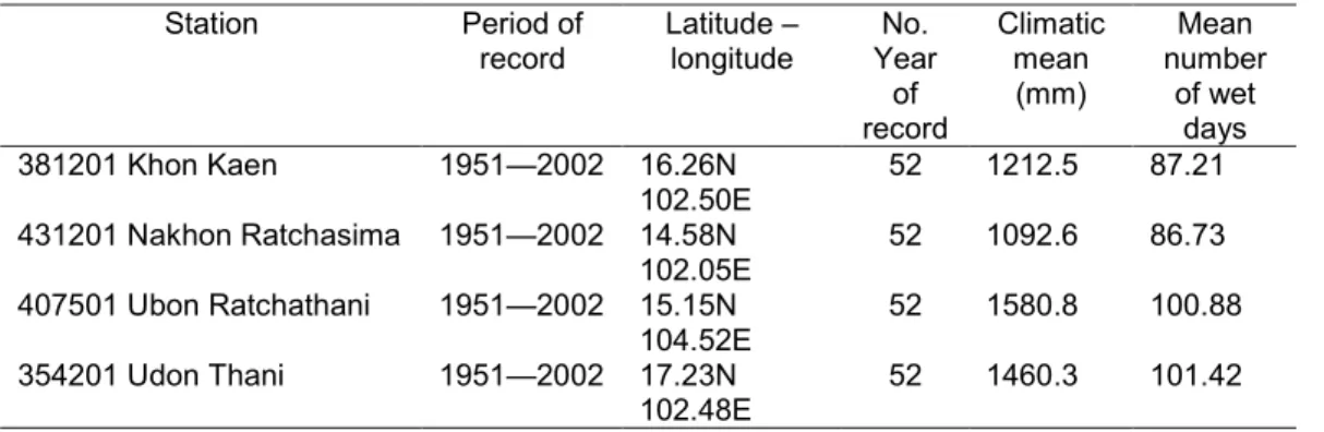
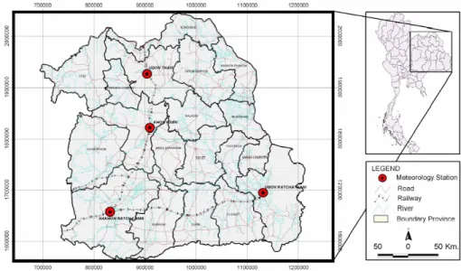
The point rainfall data for the 1951–2002 records from 4 gauging stations distributed over the northeastern part of Thailand were analyzed using the Downscaled Rainfall Prediction Model (DRPM). The selected rainfall stations are part of the Thai

Meteoro-10

logical Department (TMD). Details are shown in Fig. 1 and Table 1.

3. Applied theory and model structure

The basic process of the model developed is the coupling of a wavelet filter with the AR model. The process is divided into 2 steps: the annual prediction step and the downscaling step. In the downscaling step, a unit disaggregation curve (UDC) was

15

constructed to demonstrate the pattern of rainfall distribution. This unit curve can be applied to annual data to generate the monthly data.

3.1. Coupling of the autoregressive model with a wavelet filter

Generally, a signal or function f (t) can be expressed in linear decomposition (Burrus et al., 1998) by

20

f (t)=X

`

(5)

HESSD

Full Screen / Esc

EGU

where ` is an integer index for the finite sum (`=1, 2,. . . , `) or infinite sum (`=1, 2,. . . , ∞). a_` are the real valued expansion coefficients, and ψ_`(t) are the set of real valued functions of t called the expansion set. For the wavelet a two parameter system is constructed and the Eq. (1) becomes

f (t)=X k X j a_j,kψ_j,k(t) , (2) 5

where j and k are integer indices and the ψ_j,k(t) are the basis expansion functions of the mother wave ψ (t). The set of expansion coefficients a_j,k is called a discrete wavelet transform (DWT) of f (t) and Eq. (2) is the inverse transform. A wavelet sys-tem is a two-dimensional expansion set (basis) for some class of one-dimensional sig-nal. The wavelet expansion provides a time-frequency localization of the sigsig-nal.

First-10

generation wavelet systems are generated from a single scaling function (wavelet) by simple scaling and translation. The two dimensional parameterization is achieved from the function (mother wave) ψ (t) by

ψ_j,k(t)= 2j /2ψ (2jt− k) , (3)

where the factor 2j /2 maintains a constant norm independence of scale j . This

pa-15

rameterization of the time or space location by k and the frequency or the logarithm of scale by j turns out to be effective.

In order to generate a set of expansion functions, the signal can be represented by the series

f (t)=X

j,k

a_j,k2j /2ψ (2jt− k) . (4)

20

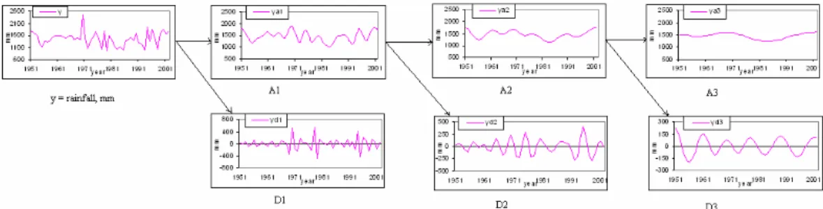
An efficient way to implement DWT is to use a filter process. Normally, the low-frequency content of the signal (approximations, A) is the most important part. It demonstrates the signal identity. The high-frequency component (detail, D) is nuance. The original signal, S, passes through two complementary filters and emerges as two

(6)

HESSD

Full Screen / Esc

EGU

signals of A and D. Figure 2 shows the rainfall series with a 1–3 layer filter where A and D are separated. By applying the historical rainfall sequences with this filter, both the A and D series was analyzed separately with AR for the step of annual rainfall prediction. The autoregressive (AR) model has been extensively applied to hydrology and water resources analysis. The AR is intuitive time dependent model, where the value of a

5

variable at the present time depends on the values at the previous time. AR models may have constant parameters, parameters varying with time or a combination of both. For AR with constant parameters, a stationary time series yt normally distributed with mean µ and variance σ2, the AR of order p, denoted by AR (p), can be represented as: 10 y_t= µ + φ₁(y_t₋₁− µ)+ .... + φp(yt−p− µ)+ εt (5) y_t= µ + p X j=1 φ_j(y_t_−j− µ)+ εt, (6)

where yt is the time dependent series and ε_t is the time independent series which is uncorrelated with yt. The series of yt is also normally distributed with the mean zero and variance σ2_ε. The coefficients φ₁,. . . , φ_p are called autoregressive coefficients.

15

Various forms of AR models, which have been used in the field of stochastic hydrology, represent the same autoregressive process. (Fiercing and Jackson, 1971; Yevjevich, 1972; Box and Jenkins, 1972) In order to yield a normal series, it is necessary to trans-form the series before carrying out the analysis. Instead of the conventional transfor-mation of logarithm transform or z transform, the wavelet filter was coupled with the AR

20

model in this study.

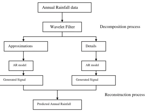
The process for annual rainfall prediction is shown in Fig. 3. The fourth order of AR was used to generate both the A and D series and the predicted annual rainfall obtained from reconstruction from these generated series.

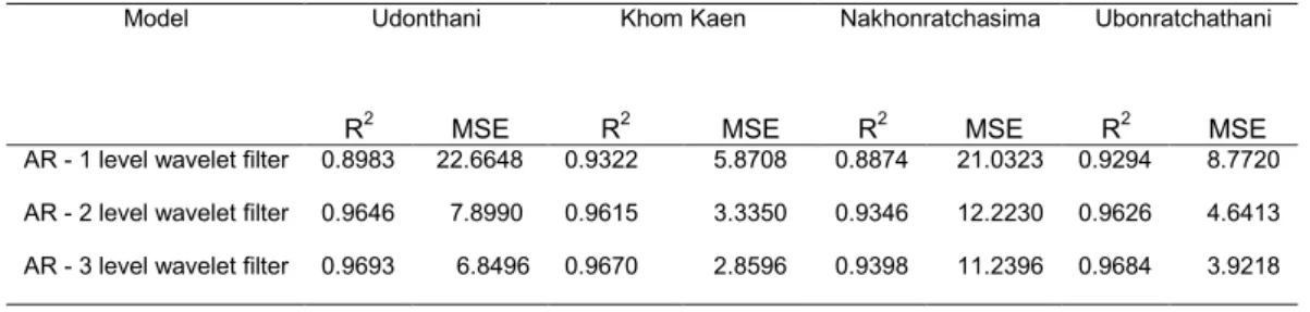
The R-square (R2) and mean square error (MSE) obtained from the simulation of the

25

(7)

HESSD

Full Screen / Esc

EGU

number of rainy days per year and the annual rainfall, respectively.

With the high level of R-square in all levels of wavelet filter used, it can be stated that the process is able to describe the annual series of rainfall characteristics. Therefore, further study was conducted to analyze the pattern of rainfall distribution over a year in order to develop the process of downscaled rainfall prediction.

5

3.2. Unit Disaggregation Curve (UDC)

The basic concept of disaggregation in terms of a linear dependence model (Valencia and Schaake, 1973) can easily be expressed as:

Y = AX + Bε , (7)

where Y is the current observation of the series being generated (subseries or monthly

10

series in this study) and depends on the current values of the X series (key series or annual series); A and B are the parameters; and ε represents the stochastic term. A study was carried out under the concept of the linear relationship between annual and monthly series. The distribution of rainfall over a year was obtained from analyzing the historical monthly rainfall series. As the monthly series of rainfall is also a time

15

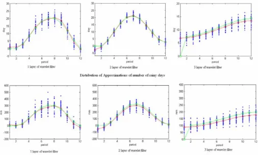
series composed of deterministic and stochastic components, the series was applied freshly through a wavelet filter in order to separate the Approximation (A) and Details (D). Then, both A and D were analyzed using the AR model. A demonstrates the signal characteristic, whereas D is the nuance of the signal. Therefore, the pattern of monthly rainfall distribution is obtained from A. Figure 4 shows the distribution of A for number

20

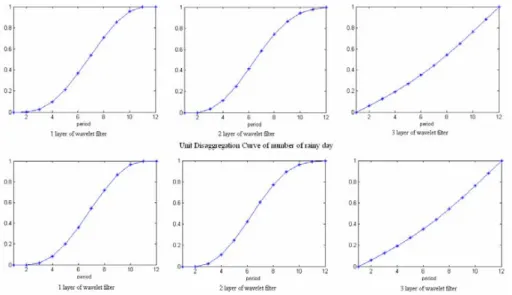
of rainy days and rainfall within a year obtained from 52 year records of rainfall. The figure illustrates that the signal identity disappeared when passing through a 3 layer wavelet filter. With the polynomial fitting and mean value curve, the distribution curve of Approximations was obtained.

The unit disaggregation curve is constructed from the cumulative value of the

distri-25

bution curve of Approximations and alters to a unit curve. Figure 5 shows the UDC for the number of rainy days and the rainfall of the Ubon Ratchathani station. The obtained

(8)

HESSD

Full Screen / Esc

EGU

UDC was applied directly to the predicted annual rainfall to generate monthly rainfall. The process of monthly rainfall prediction is shown in Fig. 6. The process is similar to the annual rainfall prediction when A and D are generated separately. For the monthly rainfall prediction, D of the annual series is considered in detail. The reconstruction process of the monthly signal is done by merging the generated A with generated D;

5

therefore, the D or nuance already existed in the generated series. That is why the D of the annual rainfall has to be eliminated before conducting the downscaled process to predict the monthly rainfall.

4. Result and discussion

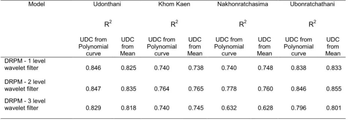
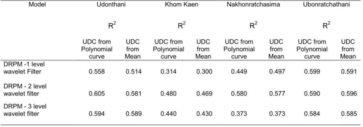
The simulation was undertaken using the 52 year historical data of the number of rainy

10

days and rainfall. Tables 4 and 5 show the obtained R-square of the 30 year (1973– 2002) generated series compared with the historical data of number of rainy days and monthly rainfall, respectively. Figures 7 and 8 demonstrate the example graphs of the 1997–2002 generated series from the DRPM of a 1–3 level filter for the number of rainy days and monthly rainfall, respectively. With high R-square values of 0.760–

15

0.855, the DRPM with a 2 level wavelet filter and UDC from both a polynomial curve and a mean value curve are appropriate to describe the characteristics of number of rainy day series. In case of the rainfall series simulation, the DRPM with a 2 level wavelet filter and UDC from both polynomials and mean values provide the R-square values of 0.469–0.605 which can be used to describe the pattern of rainfall series, as

20

well.

Further study was carried out to utilize DRPM as the rainfall prediction for the year 2002 compared with the records. Tables 6 and 7 show the obtained R-square for predicted rainfall and historical data. Figures 9 and 10 illustrate the distribution pattern for predicted values compared with the records in year 2002. It can be seen that

25

the DRPM with a 2 level wavelet filter is the most appropriate process for the rainfall prediction model.

(9)

HESSD

Full Screen / Esc

EGU

5. Conclusions

DRPM is a multi-step prediction model, developed from coupling the AR model with a wavelet filter. The construction of UDC is to study the pattern of rainfall distribution within a year to apply for downscaling rainfall from the large time scale to a finer scale. Although, the DRPM can be applied for both the number of rainy days per month and

5

monthly rainfall, the DRPM provides a better result when applied to the number of rainy days. However, the DRPM can be utilized for predicting annual and monthly rainfall reasonably well to serve the purpose of water resources planning.

References

Box, G. E. P. and Jenkins, G.: Time series analysis, forecasting and control, Holden-Day Inc., 10

San Francisco, 1970.

Burrus, C. S., Gopinath, R. A., and Guo, H.: Introduction to wavelets and wavelet transforms, Prentice-Hall International Inc., Texas, 1998.

Carlson, R. F., MacCormick, A. J. A., and Watts, D. G.: Application of linear model to four annual stream flow series, J. Water Resour. Res., 6, 4, 1070–1078, 1970.

15

Feircing, M. B. and Jackson, B. B.: Synthetic hydrology monograph no. 1., American geophys-icaal Union, Washington D.C., 1971.

Hoshi, K. and Burges, S. J.: Disaggregation of streamflow volumes, J. of Hydrology, Div., ASCE, 105, 27–41, 1979.

Huang, M.-C.: Wave parameters and functions in wavelet analysis, Ocean Engineering, 31, 1, 20

111–125, 2004.

Jury, M. R. and Melice J.-L.: Analysis of Durban rainfall and Nile river flow 1871–1999, Theor. Appl. Climatol., 67, 161–169, 2000.

Koutsoyiannis, D., A stochastic disaggregation method for design strom and flood synthesis, J. of Hydrology, 156, 193–225, 1994.

25

Koutsoyiannis, D.: Coupling stochastic models of different time scales, J. Water Resour. Res., 37, 2, 379–391, 2001.

(10)

HESSD

Full Screen / Esc

EGU

Lau, K. M. and Weng, H. Y.: Climate signal detection using wavelet transform: how to make a time series sing, Bull. Amer. Meteor Soc., 76, 2391–2402, 1995.

Mallat, S.: A wavelet tour of signal processing, San Diego, CA: Academic Press, 1998.

Matalas, N. C. and Willis, J. R.: Statistical properties of multivariate fractional noise processes, J. Water Resour. Res., 7, 6, 1460–1468, 1971.

5

Massel, S. R.: Wavelet analysis for processing of ocean surface wave records, Ocean Engi-neering, 28, 957–987, 2001.

Mejia, J. M. and Rousselle, J.: Disaggregation models in hydrology revisited, J. Water Resour. Res., 12, 2, 185–186, 1976.

Salas, J. D. Delleur, J. W., Yevjevich, V., and Lane, W. L.: Applied modeling of hydrological time 10

series, Book Crafters, Inc. Michigan, 1985.

Stedinger, J. R. and Vogel R. M.: Disaggregation procedures for generating serially corrected flow vector, J. Water Resour. Res., 20, 1, 47–56, 1984.

Teisseire, L. M., Delafoy, M. G., Jordan, D. A., Miksad, R. W., and Weggel, D. C.: Measurement of the instantaneous characteristics of natural response modes of a spar platform subjected 15

to irregular wave loading, International Journal of offshore and polar Enigineering, 12, 1, 16–24, 2002.

Thomas, H. A. and Fiering, M. B.: Mathematic synthesis of streamflow sequences for analysis of river basins by simulation. In Design of water resources systems, Mass, A. et al., 459–493, Harvard University press, Massachusetts, 1962.

20

Torrence, C. and Compo, G. P.: A practical guide to wavelet analysis, Bull. Amer. Meteor. Soc., 79, 1, 61–78, 1997.

Tsui, F.-C., Li, C. C., Sun, M. et al.,: A comparative study of two biorthogonal wavelet transforms in time series prediction, IEEE, 1997.

Valencia, D. R., and Schaake, J. C. Jr.: Disaggregation processes in stochastic hydrology, J. 25

Water Resour. Res., 9, 3, 580–585, 1973.

Yevjevich, V.: Fluctuation of wet and dry years, Part 1 Hydrology paper 1, Colorado State University, Fort Collins, Colorado, 1963.

Yevjevich, V.: Stochastic processes in hydrology, Water Resources publication, Fort Collins, Colorado, 1972a.

30

Yevjevich, V.: Structural Analysis of hydrological time series, Hydrology paper, 56, Colorado State University, Fort Collins, Colorado, 1972b.

(11)

HESSD

Full Screen / Esc

EGU

Table 1. Details of 4 selected rainfall stations._{Table 1 Details of 4 selected rainfall stations}

Table 2 The simulation results of the number of rainy day per year

Table 3 The simulation result of the annual rainfall

Station Period of record Latitude – longitude No. Year of record Climatic mean (mm) Mean number of wet days 381201 Khon Kaen 1951—2002 16.26N 102.50E 52 1212.5 87.21 431201 Nakhon Ratchasima 1951—2002 14.58N 102.05E 52 1092.6 86.73 407501 Ubon Ratchathani 1951—2002 15.15N 104.52E 52 1580.8 100.88 354201 Udon Thani 1951—2002 17.23N 102.48E 52 1460.3 101.42

Udonthani Khom Kaen Nakhonratchasima Ubonratchathani Model

R2 MSE R2 MSE R2 MSE R2 MSE

AR - 1 level wavelet filter 0.8983 22.6648 0.9322 5.8708 0.8874 21.0323 0.9294 8.7720 AR - 2 level wavelet filter 0.9646 7.8990 0.9615 3.3350 0.9346 12.2230 0.9626 4.6413 AR - 3 level wavelet filter 0.9693 6.8496 0.9670 2.8596 0.9398 11.2396 0.9684 3.9218

R2 _MSE _R2 _MSE _R2 _MSE _R2 _MSE

AR - 1 level wavelet filter 0.8907 8538.1754 0.9228

5327.7085 0.8954 4554.9483 0.9210 5317.6073 AR - 2 level wavelet filter 0.9346 5110.6815 0.9568

2741.2951 0.9404 2595.1318 0.9684 2126.6607

(12)

HESSD

Full Screen / Esc

EGU

Table 2. The simulation results of the number of rainy day per year.

Table 1 Details of 4 selected rainfall stations

Table 2 The simulation results of the number of rainy day per year

Table 3 The simulation result of the annual rainfall

Station Period of record Latitude – longitude No. Year of record Climatic mean (mm) Mean number of wet days 381201 Khon Kaen 1951—2002 16.26N 102.50E 52 1212.5 87.21 431201 Nakhon Ratchasima 1951—2002 14.58N 102.05E 52 1092.6 86.73 407501 Ubon Ratchathani 1951—2002 15.15N 104.52E 52 1580.8 100.88 354201 Udon Thani 1951—2002 17.23N 102.48E 52 1460.3 101.42

AR - 1 level wavelet filter 0.8983 22.6648 0.9322 5.8708 0.8874 21.0323 0.9294 8.7720 AR - 2 level wavelet filter 0.9646 7.8990 0.9615 3.3350 0.9346 12.2230 0.9626 4.6413 AR - 3 level wavelet filter 0.9693 6.8496 0.9670 2.8596 0.9398 11.2396 0.9684 3.9218

R2 _MSE _R2 _MSE _R2 _MSE _R2 _MSE

AR - 1 level wavelet filter 0.8907 8538.1754 0.9228 5327.7085

0.8954 4554.9483

0.9210 5317.6073 AR - 2 level wavelet filter 0.9346 5110.6815 0.9568

2741.2951

0.9404 2595.1318

0.9684 2126.6607

(13)

HESSD

Full Screen / Esc

EGU

Table 3. The simulation result of the annual rainfall.

Udonthani Khom Kaen Nakhonratchasima Ubonratchathani

Model

R2_{MSE R}2_{MSE R}2_{MSE R}2_MSE

AR -1 level wavelet Filter 0.8907 8538.1754 0.9228 5327.7085 0.8954 554.9483 0.9210 5317.6073 AR - 2 level wavelet filter 0.9346 5110.6815 0.9568 2981.6889 0.9346 849.9213 0.9633 2466.7780 AR - 3 level wavelet filter 0.9425 4496.4688 0.9603 2741.2951 0.9404 595.1318 0.9684 2126.6607

(14)

HESSD

Full Screen / Esc

EGU

Table 4. Obtained R-square of 30 year generated series of number of rainy days.

Table 4 Obtained R-square of 30 year generated series of Number of rainy days

Table 5 Obtained R-square of 30 year generated series of monthly rainfall

Table 6 Obtained R-square of 2002 predicted Number of rainy days

Table 7 Obtained R-square of 2002 predicted monthly rainfall

R2 R2 R2 R2 Model UDC from Polynomial curve UDC from Mean UDC from Polynomial curve UDC from Mean UDC from Polynomial curve UDC from Mean UDC from Polynomial curve UDC from Mean DRPM - 1 level wavelet filter 0.846 0.825 0.740 0.738 0.740 0.748 0.838 0.833 DRPM - 2 level wavelet filter 0.847 0.835 0.764 0.765 0.778 0.760 0.846 0.855 DRPM - 3 level wavelet filter 0.829 0.818 0.740 0.745 0.632 0.628 0.796 0.801

R2 _R2 _R2 _R2 Model UDC from Polynomial curve UDC from Mean UDC from Polynomial curve UDC from Mean UDC from Polynomial curve UDC from Mean UDC from Polynomial curve UDC from Mean DRPM -1 level wavelet Filter 0.558 0.514 0.314 0.300 0.449 0.497 0.599 0.591 DRPM - 2 level wavelet filter 0.605 0.581 0.480 0.469 0.580 0.577 0.590 0.596 DRPM - 3 level wavelet filter 0.594 0.589 0.440 0.430 0.373 0.373 0.584 0.585

R2 _R2 _R2 _R2 Model UDC from Polynomial curve UDC from Mean UDC from Polynomial curve UDC from Mean UDC from Polynomial curve UDC from Mean UDC from Polynomial curve UDC from Mean DRPM -1 level wavelet Filter 0.840 0.851 0.657 0.762 0.589 0.666 0.840 0.851 DRPM - 2 level wavelet filter 0.901 0.913 0.674 0.709 0.715 0.727 0.901 0.913 DRPM - 3 level wavelet filter 0.884 0.888 0.327 0.376 0.640 0.649 0.884 0.888 555

(15)

HESSD

Full Screen / Esc

EGU

Table 5. Obtained R-square of 30 year generated series of monthly rainfall.

R2 _R2 _R2 _R2 Model UDC from Polynomial curve UDC from Mean UDC from Polynomial curve UDC from Mean UDC from Polynomial curve UDC from Mean UDC from Polynomial curve UDC from Mean DRPM - 1 level wavelet filter 0.846 0.825 0.740 0.738 0.740 0.748 0.838 0.833 DRPM - 2 level wavelet filter 0.847 0.835 0.764 0.765 0.778 0.760 0.846 0.855 DRPM - 3 level wavelet filter 0.829 0.818 0.740 0.745 0.632 0.628 0.796 0.801

(16)

HESSD

Full Screen / Esc

EGU

Table 6. Obtained R-square of 2002 predicted Number of rainy days.

R2 _R2 _R2 _R2 Model UDC from Polynomial curve UDC from Mean UDC from Polynomial curve UDC from Mean UDC from Polynomial curve UDC from Mean UDC from Polynomial curve UDC from Mean DRPM - 1 level wavelet filter 0.846 0.825 0.740 0.738 0.740 0.748 0.838 0.833 DRPM - 2 level wavelet filter 0.847 0.835 0.764 0.765 0.778 0.760 0.846 0.855 DRPM - 3 level wavelet filter 0.829 0.818 0.740 0.745 0.632 0.628 0.796 0.801

R2 R2 R2 R2 Model UDC from Polynomial curve UDC from Mean UDC from Polynomial curve UDC from Mean UDC from Polynomial curve UDC from Mean UDC from Polynomial curve UDC from Mean DRPM -1 level wavelet Filter 0.558 0.514 0.314 0.300 0.449 0.497 0.599 0.591 DRPM - 2 level wavelet filter 0.605 0.581 0.480 0.469 0.580 0.577 0.590 0.596 DRPM - 3 level wavelet filter 0.594 0.589 0.440 0.430 0.373 0.373 0.584 0.585

R2 R2 R2 R2 Model UDC from Polynomial curve UDC from Mean UDC from Polynomial curve UDC from Mean UDC from Polynomial curve UDC from Mean UDC from Polynomial curve UDC from Mean DRPM -1 level wavelet Filter 0.840 0.851 0.657 0.762 0.589 0.666 0.840 0.851 DRPM - 2 level wavelet filter 0.901 0.913 0.674 0.709 0.715 0.727 0.901 0.913 DRPM - 3 level wavelet filter 0.884 0.888 0.327 0.376 0.640 0.649 0.884 0.888

(17)

HESSD

Full Screen / Esc

EGU

Table 7. Obtained R-square of 2002 predicted monthly rainfall.

Figure 1 Location of the 4 selected rainfall stations

Figure 2 Rainfall series pass through 1-3 layer of wavelet filter (Udon Thani station) Figure 3 The process of coupling AR with wavelet filter for annual rainfall prediction Figure 4 Approximations distribution within a year of Ubon Ratchathani station ( : mean value, : value from polynomial fitting curve)

Figure 5 Obtained Unit Distribution Curve from polynomial fitting curve of the number of rainy days and rainfall (Ubon Ratchathani station)

Figure 6 DRPM model structure

Figure 7 The generated series of number of rainy days (1997-2002) by DRPM of 1-3 level of filter UDCMx : process of x level of wavelet filter and UDC from mean values curve

UDCPx : process of x level of wavelet filter and UDC from Polynomials fitting curve Real : historical records

Figure 8 The generated series of rainfall (1997-2002) by DRPM of 1-3 level of filter UDCMx : process of x level of wavelet filter and UDC from mean values curve UDCPx : process of x level of wavelet filter and UDC from Polynomials fitting curve Real : historical records

(18)

HESSD

Full Screen / Esc

EGU Figure 1 Location of the 4 selected rainfall stations

Table 1 Details of 4 selected rainfall stations

3. Applied theory and model structure

The basic process of the model developed is the coupling of a wavelet filter with the AR model. The process is divided into 2 steps: the annual prediction step and the downscaling step. In the downscaling step, a unit disaggregation curve (UDC) was constructed to demonstrate the pattern of rainfall distribution. This unit curve can be applied to annual data to generate the monthly data.

3.1 Coupling of the autoregressive model with a wavelet filter

Generally, a signal or function f(t) can be expressed in linear decomposition (Burrus C.S. et.al.,1998) by

∑

= l l l ) ( ) (t a t f ψ (1)

where l is an integer index for the finite sum (_{l = 1,2,.. l ) or infinite sum( l = 1,2,..} ∞ ). a are the real valued expansion _l

coefficients, and ψ_l(t)are the set of real valued functions of t called the expansion

Station Period of record Latitude – longitude No. Year of record Climatic mean (mm) Mean number of wet days 381201 Khon Kaen 1951-2002 16.26N 102.50E 52 1212.5 87.21 431201 Nakhon Ratchasima 1951-2002 14.58N 102.05E 52 1092.6 86.73 407501 Ubon Ratchathani 1951-2002 15.15N 104.52E 52 1580.8 100.88 354201 Udon Thani 1951-2002 17.23N 102.48E 52 1460.3 101.42 Fig. 1. Location of the 4 selected rainfall stations.

(19)

HESSD

Full Screen / Esc

EGU

system is constructed and the equation (1)

becomes

) ( ) (t a , , t f j k k j k j

ψ

∑∑

=

(2)

where j and k are integer indices and the

)

(

,k

t

j

ψ

are the basis expansion functions

of the mother wave

ψ

(t).

The set of

expansion coefficients

a

_j_,_k

is called a

discrete wavelet transform (DWT) of f(t)

and equation (2) is the inverse transform.

A wavelet system is a two-dimensional

expansion set (basis) for some class of

one-dimensional signal. The wavelet

expansion provides a time-frequency

localization of the signal. First-generation

wavelet systems are generated from a

single scaling function (wavelet) by simple

scaling and translation. The two

dimensional parameterization is achieved

from the function (mother wave)

ψ

(t)

by

)

2 (

2 )

(

/2 ,

t

k

j j k j

=

ψ

−

ψ

(3)

where the factor 2

j/2

maintains a constant

norm independence of scale j. This

parameterization of the time or space

location by k and the frequency or the

logarithm of scale by j turns out to be

effective.

In order to generate a set of

expansion functions, the signal can be

represented by the series

∑

−

=

k j j j k j

t

k

a

t

f

, 2 / ,

2 (

2 )

)

(

ψ

(4)

An efficient way to implement

DWT is to use a filter process. Normally,

the low-frequency content of the signal

(approximations, A) is the most important

part. It demonstrates the signal identity.

The high-frequency component (detail, D)

is nuance. The original signal, S, passes

through two complementary filters and

emerges as two signals of A and D. Figure

2 shows the rainfall series with a 1-3 layer

filter where A and D are separated. By

applying the historical rainfall sequences

with this filter, both the A and D series

was analyzed separately with AR for the

step of annual rainfall prediction.

Figure

2 Rainfall series pass through 1-3 layer of wavelet filter (Udon Thani station)

The autoregressive (AR) model has

been extensively applied to hydrology and

water resources analysis. The AR is

intuitive time dependent model, where the

value of a variable at the present time

depends on the values at the previous time.

AR models may have constant parameters,

parameters varying with time or a

combination of both. For AR with constant

parameters, a stationary time series y

t

normally distributed with mean

µ

and

variance

σ

2

, the AR of order p, denoted by

AR (p), can be represented as:

t p t p t t y y y =µ+φ₁( ₋₁−µ)+....+φ ( ₋ −µ)+ε

(5)

t j t p j j t

y

=

µ

+

φ

₋

−

µ

+

ε

=

∑

(

)

1

(6)

where y

t

is the time dependent series and

ε

_t

is the time independent series which is

uncorrelated with y

t

. The series of y

t

is also

normally distributed with the mean zero

and variance

σ

ε2

. The coefficients

φ

1

,…,

φ

p

Fig. 2. Rainfall series pass through 1–3 layer of wavelet filter (Udon Thani station).

(20)

HESSD

Full Screen / Esc

EGU

are called autoregressive coefficients.

Various forms of AR models, which have

been used in the field of stochastic

hydrology, represent the same

autoregressive process. (Fiercing and

Jackson, 1971; Yevjevich, 1972; and Box

and Jenkins, 1972) In order to yield a

normal series, it is necessary to transform

the series before carrying out the analysis.

Instead of the conventional transformation

of logarithm transform or z transform, the

wavelet filter was coupled with the AR

model in this study.

The process for annual rainfall

prediction is shown in Figure 3. The fourth

order of AR was used to generate both the

A and D series and the predicted annual

rainfall obtained from reconstruction from

these generated series.

Figure 3 The process of coupling AR with wavelet filter for annual rainfall prediction

The R-square (R

2

) and mean square

error (MSE) obtained from the simulation

of the annual rainfall series using AR with

a 1-3 layer filter is shown in tables 2 and 3

for the number of rainy days per year and

the annual rainfall, respectively.

Table 2 The simulation results of the number of rainy day per year

Model

AR -1 level wavelet Filter 0.8983 22.6648 0.9322 5.8708 0.8874 21.0323 0.9294 8.7720 AR - 2 level wavelet filter 0.9646 7.8990 0.9615 3.3350 0.9346 12.2230 0.9626 4.6413 AR - 3 level wavelet filter 0.9693 6.8496 0.9670 2.8596 0.9398 11.2396 0.9684 3.9218

Annual Rainfall data

Wavelet Filter

Approximations Details

AR model AR model

Generated Signal Generated Signal

Predicted Annual Rainfall

Decomposition process

Reconstruction process

Fig. 3. The process of coupling AR with wavelet filter for annual rainfall prediction.

(21)

HESSD

Full Screen / Esc

EGU

Figure 4 Approximations distribution within a year of Ubon Ratchathani station ( : mean value, : value from polynomial fitting curve)

Figure 5 Obtained Unit Distribution Curve from polynomial fitting curve of the number of rainy days and rainfall (Ubon Ratchathani station)

Fig. 4. Approximations distribution within a year of Ubon Ratchathani station (red line: mean value, green line: value from polynomial fitting curve).

(22)

HESSD

Full Screen / Esc

EGU

Figure 4 Approximations distribution within a year of Ubon Ratchathani station ( : mean value, : value from polynomial fitting curve)

Figure 5 Obtained Unit Distribution Curve from polynomial fitting curve of the number of rainy days and rainfall (Ubon Ratchathani station)

Fig. 5. Obtained Unit Distribution Curve from polynomial fitting curve of the number of rainy days and rainfall (Ubon Ratchathani station).

(23)

HESSD

Full Screen / Esc

EGU

4. Result and discussion

The simulation was undertaken using the 52 year historical data of the number of rainy days and rainfall. Tables 4 and 5 show the obtained R-square of the 30 year (1973-2002) generated series compared with the historical data of number of rainy days and monthly rainfall, respectively. Figures 7 and 8 demonstrate the example graphs of the 1997-2002 generated series from the DRPM of a 1-3 level filter for the number of rainy days and monthly rainfall, respectively. With high R-square values of 0.760-0.855, the DRPM with a 2 level wavelet filter and UDC from both a polynomial curve and a mean value curve are appropriate to describe the characteristics of number of rainy day series. In case of the rainfall

series simulation, the DRPM with a 2 level wavelet filter and UDC from both polynomials and mean values provide the R-square values of 0.469-0.605 which can be used to describe the pattern of rainfall series, as well.

Further study was carried out to utilize DRPM as the rainfall prediction for the year 2002 compared with the records. Tables 6 and 7 show the obtained R-square for predicted rainfall and historical data. Figures 9 and 10 illustrate the distribution pattern for predicted values compared with the records in year 2002. It can be seen that the DRPM with a 2 level wavelet filter is the most appropriate process for the rainfall prediction model.

Sub period Rainfall records

Wavelet Filter

Details

AR model

Generated Series

Annual Rainfall data

Wavelet Filter

Approximations Details

AR model

Generated Signal Approximatio

Polynomial Fitting/ Mean value

Distribution Curve with Disaggregation Eqn

Aggregate Curve (Cumulative Curve)

Unit Disaggregation Curve (UDC) _{Predicted Annual Rainfall}

Aggregation Curve for Predicted Annual Rainfall

Predicted Sub period Rainfall

Eliminate

Fig. 6. DRPM model structure.

(24)

HESSD

Full Screen / Esc

EGU Table 4 Obtained R-square of 30 year generated series of Number of rainy days

Figure 7 The generated series of number of rainy days (1998-2002) by DRPM of 1-3 level of filter UDCMx : process of x level of wavelet filter and UDC from mean values

UDCPx : process of x level of wavelet filter and UDC from Polynomials fitting curve Real : historical records

Fig. 7. The generated series of number of rainy days (1997–2002) by DRPM of 1–3 level of filter. UDCMx: process of x level of wavelet filter and UDC from mean values curve. UDCPx: process of x level of wavelet filter and UDC from Polynomials fitting curve. Real: historical records.

(25)

HESSD

Full Screen / Esc

EGU

Figure 8 The generated series of rainfall (1998-2002) by DRPM of 1-3 level of filter UDCMx : process of x level of wavelet filter and UDC from mean values

UDCPx : process of x level of wavelet filter and UDC from Polynomials fitting curve Real : historical records

R2 _R2 _R2 _R2 Model UDC from Polynomial curve UDC from Mean UDC from Polynomial curve UDC from Mean UDC from Polynomial curve UDC from Mean UDC from Polynomial curve UDC from Mean DRPM -1 level wavelet Filter 0.288 0.284 0.377 0.569 0.522 0.591 0.704 0.705 DRPM - 2 level wavelet filter 0.668 0.631 0.690 0.697 0.500 0.506 0.788 0.790 DRPM - 3 level wavelet filter 0.418 0.355 0.192 0.202 0.396 0.396 0.688 0.677 Fig. 8. The generated series of rainfall (1997–2002) by DRPM of 1–3 level of filter. UDCMx: process of x level of wavelet filter and UDC from mean values curve. UDCPx: process of x level of wavelet filter and UDC from Polynomials. fitting curve. Real: historical records.

(26)

HESSD

Full Screen / Esc

EGU

Figure 9 The predicted number of rainy days in year 2002 by DRPM of 1-3 level of filter

UDCMx : process of x level of wavelet filter and UDC from mean values

UDCPx : process of x level of wavelet filter and UDC from Polynomials fitting curve Real : historical records

Figure 10 The predicted number of rainfall in year 2002 by DRPM of 1-3 level of filter

UDCPx : process of x level of wavelet filter and UDC from Polynomials fitting curve

Real : historical records

Fig. 9. The predicted number of rainy days in the year 2002 by DRPM of 1–3 level of filter. UDCMx : process of x level of wavelet filter and UDC from mean values curve. UDCPx: process of x level of wavelet filter and UDC from Polynomials fitting curve. Real: historical records.

(27)

HESSD

Full Screen / Esc

EGU

Figure 9 The predicted number of rainy days in year 2002 by DRPM of 1-3 level of filter

UDCPx : process of x level of wavelet filter and UDC from Polynomials fitting curve Real : historical records

Figure 10 The predicted number of rainfall in year 2002 by DRPM of 1-3 level of filter

UDCPx : process of x level of wavelet filter and UDC from Polynomials fitting curve

Real : historical records

Fig. 10. TThe predicted number of rainfall in the year 2002 by DRPM of 1–3 level of filter. UDCMx: process of x level of wavelet filter and UDC from mean values curve. UDCPx: process of x level of wavelet filter and UDC from Polynomials fitting curve. Real: historical records.