HAL Id: hal-00295362
https://hal.archives-ouvertes.fr/hal-00295362
Submitted on 21 Nov 2003
HAL is a multi-disciplinary open access
archive for the deposit and dissemination of
sci-entific research documents, whether they are
pub-lished or not. The documents may come from
teaching and research institutions in France or
abroad, or from public or private research centers.
L’archive ouverte pluridisciplinaire HAL, est
destinée au dépôt et à la diffusion de documents
scientifiques de niveau recherche, publiés ou non,
émanant des établissements d’enseignement et de
recherche français ou étrangers, des laboratoires
publics ou privés.
Climatological aspects of aerosol optical properties in
Northern Greece
E. Gerasopoulos, M. O. Andreae, C. S. Zerefos, T. W. Andreae, D. Balis, P.
Formenti, P. Merlet, V. Amiridis, C. Papastefanou
To cite this version:
E. Gerasopoulos, M. O. Andreae, C. S. Zerefos, T. W. Andreae, D. Balis, et al.. Climatological aspects
of aerosol optical properties in Northern Greece. Atmospheric Chemistry and Physics, European
Geosciences Union, 2003, 3 (6), pp.2025-2041. �hal-00295362�
Atmos. Chem. Phys., 3, 2025–2041, 2003
www.atmos-chem-phys.org/acp/3/2025/
Atmospheric
Chemistry
and Physics
Climatological aspects of aerosol optical properties in Northern
Greece
E. Gerasopoulos1, 2, M. O. Andreae2, C. S. Zerefos1, T. W. Andreae2, D. Balis1, P. Formenti3, P. Merlet2, V. Amiridis1, and C. Papastefanou4
1Laboratory of Atmospheric Physics, Physics Department, Aristotle University of Thessaloniki, P.O. Box 149, GR-54124
Thessaloniki, Greece
2Max Planck Institute for Chemistry, Biogeochemistry Department, P.O. Box 3060, D-55020 Mainz, Germany 3Centre of Geophysics of ´Evora, Universidade de ´Evora, Rua R. Ramalho, 59, P-7000-532 Evora, Portugal 4Nuclear Physics Department, Aristotle University of Thessaloniki, GR-54124 Thessaloniki, Greece
Received: 27 November 2002 – Published in Atmos. Chem. Phys. Discuss.: 15 April 2003 Revised: 6 November 2003 – Accepted: 7 November 2003 – Published: 21 November 2003
Abstract. Measurements of aerosol optical proper-ties (aerosol optical depth, scattering and backscatter-ing coefficients) have been conducted at two ground-based sites in Northern Greece, Ouranoupolis (40◦230N, 23◦570E, 170 m a.s.l.) and Thessaloniki (40◦380N, 22◦570E, 80 m a.s.l.), between 1999 and 2002. The frequency distri-butions of the observed parameters have revealed the pres-ence of individual modes of high and low values, indicating the influence from different sources. At both sites, the mean aerosol optical depth at 500 nm was 0.23. Values increase considerably during summer when they remain persistently between 0.3 and 0.5, going up to 0.7–0.8 during specific cases. The mean value of 65±40 Mm−1of the particle
scat-tering coefficient at 550 nm reflects the impact of continen-tal pollution in the regional boundary layer. Trajectory anal-ysis has shown that higher values of aerosol optical depth and the scattering coefficient are found in the east sector (former Soviet Union countries, eastern Balkan countries), whereas cleaner conditions are found for the NW direction. The influence of Sahara dust events is clearly reflected in the
˚
Angstr¨om exponents. About 45–60% of the observed diur-nal variation of the optical properties was attributed to the growth of aerosols with humidity, while the rest of the vari-ability is in phase with the evolution of the sea-breeze cell. The contribution of local pollution is estimated to contribute 35±10% to the average aerosol optical depth at the Thessa-loniki site during summer. Finally, the aerosol scale height (aerosol optical depth divided by scattering coefficient) was found to be related to the height of the boundary layer with values between 0.5–1 km during winter and up to 2.5–3 km during summer.
Correspondence to: E. Gerasopoulos
1 Introduction
The role of aerosols in a changing climate has been under scrutiny during the past decades (e.g. Coakley et al., 1983; Andreae, 1995; Penner et al., 2001; Haywood and Boucher, 2000). Depending on their intrinsic properties, especially the single scattering albedo, aerosols can cause either cool-ing or warmcool-ing of the atmosphere, in contrast to the green-house gases which only cause warming. Nevertheless, the “level of scientific understanding” concerning the various cli-matic effects of atmospheric aerosols is still very inadequate (Houghton et al., 2001; Shine and Forster, 1999).
In the last decade, a substantial number of experimental studies on aerosols have focused on the eastern Mediter-ranean area (Luria et al., 1996; Pinker et al., 1997; Mi-halopoulos et al., 1997; Paronis et al., 1998; Papayiannis et al., 1998; Ichoku et al., 1999; Andreae et al., 2002; Formenti et al., 2001a, b, 2002a, b; Lelieveld et al., 2002; Kouvarakis et al., 2002). This is because of the maximum in the net di-rect radiative forcing by sulfate aerosols predicted to occur in this region by various models (Charlson et al., 1991; Kiehl and Rodhe, 1995; Boucher and Anderson, 1995). Accu-mulation of aerosols and enhanced backscattering is favored by the meteorological conditions prevailing over the eastern Mediterranean, namely sparse cloudiness and prolonged ex-posure to solar radiation. Concentrations of important trace gases and aerosols are typically factors of 2 to 10 higher over the Mediterranean than over the North Pacific Ocean, expected to be the least polluted environment at low northern latitudes (Lelieveld et al., 2002). Within the eastern Mediter-ranean, the Aegean sea and the coastal part of continental Greece are in a “key” geographical position where aerosols from different sources converge, namely maritime aerosols
2026 E. Gerasopoulos et al.: Aerosol optical properties in Northern Greece from sea spray; mineral dust from North Africa; and
anthro-pogenic aerosols from the highly populated urban centers and industrial areas, as well as seasonal biomass burning (For-menti et al., 2002a; 2002b). In the lower troposphere over the Mediterranean, European pollution is mainly responsi-ble for the reduction of air quality, particularly during sum-mer, whereas in the free troposphere pollution is largely de-termined by transboundary and even intercontinental trans-port (Lelieveld et al., 2002; Balis et al., 2003; Eisinger and Burrows, 1998; Zerefos et al., 2000).
Furthermore, the impact of aerosols on the photochemical activity and thus on the air quality of the region is very impor-tant and has been studied extensively during the Photochem-ical Activity and Ultraviolet Radiation (PAUR) campaigns (Zerefos et al., 2002) that took place in the Northern Aegean (1996) and on Crete (1999). These studies showed that var-ious (in type and quantity) aerosols can modulate the solar UV radiation reaching the Earth’s surface in such a way that it can mask changes induced from total ozone itself (Kylling et al., 1997). Moreover, in the presence of high tropospheric ozone (Kourtidis et al., 2002) and high absorbing aerosols from the Sahara desert, reduction in the UV and in associ-ated photolysis rates have been measured even if total ozone decreases (Balis et al., 2002).
In this paper, we present the results of an extended time series (1999–2002) of measurements of the optical char-acteristics of aerosols (optical depth, scattering and back-scattering coefficient, ˚Angstr¨om exponent, backscatter ra-tio), and thereby establish a climatology of aerosols in the region. Following the description of the instrumentation and data analysis methodology (Sect. 2), the basic statistical properties of the measured and calculated quantities are pre-sented together with their frequency distributions (Sect. 3.1). In Sect. 3.2, the source distribution of aerosols with differ-ent properties is investigated via air mass trajectory anal-ysis. The temporal variation of aerosol optical properties for two time-scales, seasonal and diurnal, is then described (Sects. 3.3, 3.4, respectively), and finally an estimation of the contribution of local pollution sources (Sect. 4.1) and of the aerosol scale height (Sect. 4.2) is attempted. The follow-ing notation for the optical properties of aerosols will be used in the text:
AOD=aerosol optical depth,
˚aτ= ˚Angstr¨om exponent calculated from aerosol optical
depths at different wavelengths, ˚aτ= −ln[τ (λ1)/τ (λ2)]/ln(λ1/λ2)
(e.g. Weller et al., 1998), σsp= scattering coefficient,
σbsp= back-scattering coefficient,
˚aσ= ˚Angstr¨om exponent calculated from scattering
coeffi-cients at different wavelengths, β=backscatter ratio (σbsp/σsp).
2 Instrumentation and methodology
2.1 Site description
Measurements of aerosol optical properties have been con-ducted at two ground-based sites in Northern Greece between 1999 and 2002. The first station is situated in the region of Ouranoupolis (Mount Athos Observatory, MAO, 40◦230N, 23◦570E, 170 m a.s.l.), a rural area in the Chalkidiki penin-sula, 100 km east of Thessaloniki, the closest major city with a population of approximately 1 million. The second sta-tion is located in an urban setting at the Laboratory of At-mospheric Physics in Thessaloniki (LAP, 40◦380N, 22◦570E, 80 m a.s.l.). Both sites face the Aegean Sea to the south and are situated along the expected pathway through which pollu-tion from central and eastern Europe influences aerosol load-ing over the Eastern Mediterranean.
2.2 Instrumentation
At MAO, a multi-filter rotating shadowband radiometer (MFR-7 Yankee Env. System Inc., Turner Falls, MA) has been providing 1-min average aerosol optical depths (AOD) at five wavelengths (415, 501, 615, 675 and 867 nm) since June 1999, with a gap from September 2000 until June 2001 due to instrument malfunctioning. A three wavelength (450, 550 and 700 nm) integrating nephelometer (TSI 3563, TSI Inc., St Paul, MN) has been also providing continuous mea-surements (2-min resolution) of the particle light scattering coefficients for both total scattering (σsp) and back-scattering
(σbsp) for the same period, with minor gaps from
Septem-ber to middle NovemSeptem-ber 1999 and from April to July 2001. A second multi-filter rotating shadowband radiometer of the same type has been operating at LAP since February 2001. Valid measurements from the MFR were obtainable during day-time under clear sky conditions only. Gaps in the time series are associated with either total cloudiness, enhanced during the fall-winter period, or with power failures at Oura-noupolis after severe weather phenomena (thundershowers, snowfall etc.). Regular calibration checks and instrument maintenance have been performed during the period of op-eration.
2.3 Methods
A detailed description of the operation principles of the MFR can be found in Harrison et al. (1994a), and a consider-able number of publications have suggested various algo-rithms for the retrieval of aerosol optical depths from mea-surements of the direct solar irradiance (e.g. Bruegge at al., 1992; Michalsky et al., 2001; Alexandrov et al., 2002a). The procedure followed in the present study is described below:
At first, the Langley linear regression technique (Harrison et al., 1994b) was applied to morning and afternoon data with airmass, m, between 2 and 6. This provided us with the so-lar constant Ioestimated from the intercept of the regression
E. Gerasopoulos et al.: Aerosol optical properties in Northern Greece 2027
Table 1. Basic statistical quantities from daily values for: a) aerosol optical depth (AOD) calculated at MAO (June 1999–August 2000
and July 2001–Mar 2002) and LAP (February 2001–March 2002), b) scattering (σsp) and backscattering (σbsp) coefficients at MAO (June
1999–March 2002), c) ˚Angstr¨om exponents from optical depths ( ˚aτ) and scattering coefficients ( ˚aσ), and backscatter ratio (β). Averages are
accompanied by their standard deviation. Note that no direct comparison between the stations is feasible from this table since the values do not correspond to a common period (see Sect. 4.1 for a comparison).
a) AOD MAO 414 nm 500 nm 614 nm 671 nm 867 nm Average 0.30±0.16 0.23±0.13 0.17±0.10 0.15±0.08 0.11±0.06 Maximum 0.92 0.69 0.53 0.48 0.47 Minimum 0.042 0.028 0.025 0.025 0.020 LAP Average 0.32±0.20 0.23±0.15 0.14±0.10 0.11±0.09 0.10±0.07 Maximum 1.02 0.77 0.58 0.54 0.54 Minimum 0.073 0.050 0.012 0.010 0.026 b) σsp(Mm−1) σbsp(Mm−1) MAO 450 nm 550 nm 700 nm 450 nm 550 nm 700 nm Average 91±54 65±40 44±27 7.7±4.6 6.4±3.5 5.3±2.8 Maximum 337 246 161 26.0 21.1 17.4 Minimum 9.9 8.3 5.6 0.1 0.8 0.9 c) ˚aτ ˚aσ β (867 nm/414 nm) (700 nm/450 nm) 550 nm
MAO LAP MAO MAO
Average 1.4±0.4 1.6±0.3 1.7±0.4 0.1±0.02
Maximum 2.25 2.21 2.33 0.16
Minimum 0.18 0.4 −0.10 0.05
line. This procedure was applied to each clear-sky day that showed a log-linear relationship between irradiance and air-mass, regardless of the optical depth obtained from the slope of the regression line. The solar constants were then cor-rected for the Sun-Earth distance (Iqbal, 1983). The inclu-sion of periods with high amounts of aerosols over the sta-tion produced a bias in the estimates of Iothat showed up as
a positive correlation between optical depth (slope) and so-lar constant (intercept). To eliminate these biased values, a threshold value of optical depth was chosen for each wave-length, below which Io’s dependence on optical depth was
statistically non-significant. The remaining cases were fil-tered to eliminate days with significant variability of optical depth within the day, and the same days were used for all wavelengths. Finally, trend analysis on Iowas used to
deter-mine a possible physical deterioration of the filters or pho-todiode detectors, and a linear regression provided the final Io values to be used for each wavelength along the whole
period.
The Beer-Lambert-Bouguer law (I = I0·e−τ ·m) was next
applied to derive instantaneous measurements of the total tical depth (one-minute time resolution). Finally, aerosol op-tical depths (AODs) for the five wavelengths were obtained by subtracting the contribution of Rayleigh scattering and
ozone absorption from the total optical depth. The wave-length dependent optical depth of Rayleigh scattering was calculated from the formula of Hansen and Travis (1974) us-ing a time series of pressure available for Thessaloniki. The ozone optical depth was extracted using the ozone absorp-tion coefficients for each wavelength and the total column of ozone available from the operation of a double monochroma-tor Brewer ozone spectrophotometer at Thessaloniki (Bais et al., 1996), as well as from Earth-Probe Total Ozone Mapping Spectrometer (TOMS) data (http://toms.gsfc.nasa.gov). For the calculation of the airmass, m, we used the formula sug-gested by Hansen and Travis (1974). Results from different formulas (Young, 1994; Kasten and Young, 1989; Rosen-berg, 1966), also taking into account atmospheric refraction and the effects of a spherical Earth on the atmospheric path of radiance, were compared. The average percentage differ-ence of each airmass value calculated by the different for-mulae from their mean increased from 0.2% to 1.7% for the airmass range of 2–6 that we used.
From the 1-min resolution measurements those parts af-fected by cloudiness were easily identified and removed, al-though the presence of thin cirrus clouds inducing slight increase in optical depth was difficult to distinguish from changes in the atmospheric conditions due to aerosol loading.
2028 E. Gerasopoulos et al.: Aerosol optical properties in Northern Greece
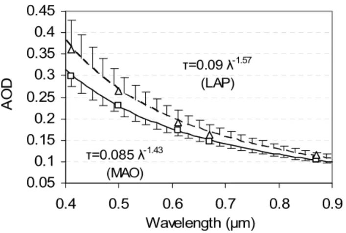
Figure 1. Wavelength dependence of aerosol optical depth, AOD. Error bars correspond to the
standard deviation of the applied power law (least squares fitting). Triangles and squares are
averages of AOD at LAP and MAO, respectively, during the period that measurements are
simultaneously available at both sites.
0.05 0.1 0.15 0.2 0.25 0.3 0.35 0.4 0.45 0.4 0.5 0.6 0.7 0.8 0.9 Wavelength (µm) AO D τ=0.09 λ-1.57 (LAP) τ=0.085 λ-1.43 (MAO)
Fig. 1. Wavelength dependence of aerosol optical depth, AOD.
Er-ror bars correspond to the standard deviation of the applied power law (least squares fitting). Triangles and squares are averages of AOD at LAP and MAO, respectively, during the period that mea-surements are simultaneously available at both sites.
For this reason, the description of cloudiness available from the Hellenic Meteorological Service at Thessaloniki helped to clarify the origins of certain diurnal disturbances. Such disturbances do not produce large changes to daily averages, but they are useful for certain case studies.
The operating principles of the TSI nephelometer as well as the methodology used to extract σsp and σbsp are
exten-sively described by Andreae et al. (2002). Corrections for the angular truncation and the nonlambertian errors were per-formed using the correction equations proposed by Ander-son and Ogren (1998). For σsp, correction was based on the
˚
Angstr¨om exponents, ˚aσ, whereas constant correction factors
were used for σbsp. To provide comparability with literature
values, we provide the resulting percentage change for our data set: For ˚aσ>1.5 the increase of σspat 550 nm stays well
within 10% and only for ˚aσ<0.5 it exceeds 20% (up to 27%)
– an average increase of 9%. The pattern is the same for the other two wavelengths, only with much higher dispersion of the values. On the other hand, σbsp are reduced by 1.8%.
The change in the recalculated value of ˚aσ(either increase or
decrease) does not exceed 10% for almost the whole range of particle size, and only for ˚aσ<0.2 an increase up to 30%
is found for a limited number of cases. Finally, backscat-ter ratios (β) decrease by 13% on average, with the decrease reaching 30–40% for ˚aσ<0.5.
3 Climatological investigation of aerosol optical proper-ties
3.1 Descriptive statistics
Before proceeding to the main analysis, we present some ba-sic statistics in order to summarize the optical properties of aerosols in our study region in the Eastern Mediterranean,
and to facilitate comparison with literature values (Table 1). A collection of literature values from previous studies is available in Formenti et al. (2001b).
The wavelength dependence of optical depth at MAO and LAP is investigated for the common period (July 2001– March 2002) using the ˚Angstr¨om’s power law approxima-tion, τ (λ)=βλ−˚a ( ˚Angstr¨om, 1929). Values of ˚a around 1.3 are representative of continental aerosols, whereas for larger aerosols (dust, seasalt) the exponents tend to zero (Michal-sky et al., 2001). As shown in Fig. 1, average ˚aτ values
for both stations, calculated from the average AOD at each wavelength ( ˚aτ=−ln[τ (λ1)/τ (λ2)]/ln(λ1/λ2), λ1=867 nm,
λ2=414 nm), are close to continental levels with values
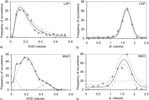
1.43±0.03 and 1.57±0.05 for MAO and LAP, respectively. The frequency distribution of all aerosol optical properties was calculated next. The resulting histograms for AOD as well as for ˚aτ are presented in Fig. 2. A rather smooth
be-havior was found for the LAP data, which allowed the fitting of a lognormal distribution for AOD and a normal distribu-tion for ˚aτ. For MAO the frequency distributions proved to
be more complicated and the estimation of statistical param-eters was subject to higher uncertainty. The choice of the distributions to be fitted was based on the fact that AOD has the natural cut-off value of zero, resulting in positive skew-ness, whereas for ˚aτ no such physical threshold exists near
the high frequency classes, and thus a normal distribution could be applied. More specifically, for LAP the lognor-mal fitting resulted into a mean AOD value of 0.126±0.006 (values after ± represent the standard error of the parame-ter estimation) and a standard deviation of 0.63±0.06. The Gaussian fitting for ˚aτ gave a mean value of 1.67±0.01 and
a standard deviation of 0.19±0.01. The distribution of ˚aτ
at MAO is flatter (low kurtosis) and a slight shift to lower values appears, with a mean of 1.57±0.05 and a standard de-viation of 0.28±0.06. Finally, a more complex distribution is found for optical depths at MAO, although once more a lognormal distribution could be fitted, leading however to enhanced uncertainty to the estimation of the parameters. Instead, three distributions were fitted in order to represent three frequency modes that seem to be consistently present. A dominant normal distribution with a mean of 0.2 (stan-dard deviation, std=0.11) explains the majority of the ob-served values, whereas for lower values a lognormal distri-bution at 0.066 (std=0.34) reflects the fact that the site is ac-tually situated at a rural area and thus this mode corresponds to background conditions. Finally, a second normal distribu-tion (mean=0.47, std=0.07) represents the higher values that possibly reflect either the fact that pollution events are more easily distinguished at this site or that data coverage is more complete during the warm season, with some gaps during the winter-spring months.
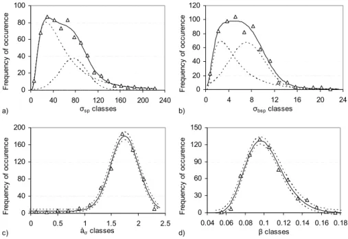
Corresponding frequency distributions were calculated for σsp, σbsp, ˚aσ and β and are presented in Fig. 3. For
both σsp and σbsp a lognormal (background conditions)
E. Gerasopoulos et al.: Aerosol optical properties in Northern Greece 2029 Figure 2. Frequency distribution of aerosol optical depth, AOD, (500 nm) and Angström
ex-ponent, åτ, (867/414 nm) at LAP (a, b) and MAO (c, d). The solid lines represent the result of
the fitting procedure on raw frequencies and the dashed lines show the standard error of each estimation. When the frequency distribution is multi-modal (c), the dashed lines represent the individual modes and the solid line the composite distribution.
0 10 20 30 40 0 0.2 0.4 0.6 0.8 AOD classes F req ue nc y o f oc cu rr en ce LAP a) 0 20 40 60 80 0 0.5 1 1.5 2 2.5 åτ classes F req ue nc y o f oc cu rr en ce LAP b) 0 10 20 30 40 50 0 0.2 0.4 0.6 0.8 AOD classes F requ en cy of o cc ur re nc e MAO c) 0 20 40 60 80 0 0.5 1 1.5 2 2.5 åτ classes F req ue nc y of oc cu rr enc e MAO d)
Fig. 2. Frequency distribution of aerosol optical depth, AOD, (500 nm) and ˚Angstr¨om exponent, ˚aτ, (867/414 nm) at LAP (a), (b) and MAO
(c), (d). The solid lines represent the result of the fitting procedure on raw frequencies and the dashed lines show the standard error of
each estimation. When the frequency distribution is multi-modal (c), the dashed lines represent the individual modes and the solid line the composite distribution.
of 28 Mm−1 (std=0.8), 76 Mm−1 (std=25) and 2.6 Mm−1 (std=0.7), 7.2 Mm−1 (std=3), respectively. Values of ˚aσ
were fitted by a normal distribution, giving a mean of 1.74±0.01 and a standard deviation of 0.26±0.02 and β ra-tios were best fitted by a lognormal distribution with a mean of 0.0961±0.0007 and a standard deviation of 0.2±0.01. 3.2 Origins of air masses arriving at the stations
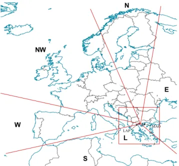
In order to investigate the source regions of particles lead-ing to elevated AOD over Northern Greece, back-trajectories (96 h) were calculated at three heights using HYSPLIT (Hybrid Single-Particle Lagrangian Integrated Trajectory Model). The heights chosen were: 1) at surface level (80 m above ground) to give representative origins of air masses for the in-situ nephelometer measurements. 2) at 1 km, which can serve as a representative height for the boundary layer in which the majority of aerosol particles is present, thus providing a good estimation of the air mass origins for the column integrated MFR measurements. 3) at 3 km for the presence of Sahara dust layers to be captured, if needed dur-ing specific case studies. We then selected sectors around the prevailing transport directions, to be used for the classifica-tion of the air mass origins.
As seen in Fig. 4, five main sectors were used: (S) southern sector, to represent the influence from the African continent, with most trajectories coming from the southwest; (W) west-ern sector, for air masses coming from either south-westwest-ern European countries or north-western African countries
hav-ing spent considerable time over the western Mediterranean or representing longer range transport from the Atlantic; (NW) northwestern sector, including the main part of central Europe; (N) Northern sector, used mainly to capture the tran-sition between the Northwestern and Eastern sectors; and (E) eastern sector, to cover air-masses originating mainly from the most eastern-northeastern part of Europe, since trajecto-ries coming from southeastern directions were quite rare. An additional sector (L) was also applied to represent those stag-nant cases when trajectories showed air masses staying for an extended period over the neighboring areas without a prevail-ing direction. When trajectories were passprevail-ing over different sectors the main sector chosen was the one over which air-masses spent most of their time, giving also additional weight to the fact that as one follows trajectories backwards there is a significant increase to their uncertainty.
Before proceeding to the more detailed investigation of the source regions, we give a brief description of the frequency and seasonality of the prevailing direction for air masses ar-riving at MAO, at both the surface and the 1 km height levels. For the days with available measurements, 40% of the trajec-tories originated from the E sector, whereas the other sectors were almost uniformly distributed with a small excess of the NW and N ones. During all seasons except winter, the E sector prevailed, and especially during summer its frequency reached 50%, while during winter the NW and N sectors re-tained each a frequency of 25–30%.
The main results of categorizing the aerosol optical prop-erties according to the origins of the air masses arriving at
2030 E. Gerasopoulos et al.: Aerosol optical properties in Northern Greece Figure 3. Frequency distribution of scattering, σsp (Mm-1), and backscattering coefficients, σbsp
(Mm-1) at 550 nm, Angström exponent, å
σ, (700/450 nm) and backscatter ratio, β, at MAO.
The solid lines represent the result of the fitting procedure on raw frequencies and the dashed lines show the standard error of each estimation. When the frequency distribution is multi-modal (a, b), the dashed lines represent the individual modes and the solid line the composite distribution. 0 40 80 120 160 200 0 0.5 1 1.5 2 2.5 åσ classes F req ue nc y of oc cu ren ce c) 0 30 60 90 120 150 0.04 0.06 0.08 0.1 0.12 0.14 0.16 0.18 β classes F req ue nc y of oc cu ren ce d) 0 20 40 60 80 100 0 40 80 120 160 200 240 σsp classes F req uen cy o f o cc urenc e a) 0 20 40 60 80 100 120 0 4 8 12 16 20 24 σbsp classes F req ue nc y of oc cu ren ce b)
Fig. 3. Frequency distribution of scattering, σsp (Mm−1), and backscattering coefficients, σbsp (Mm−1) at 550 nm, ˚Angstr¨om exponent,
˚aσ, (700/450 nm) and backscatter ratio, β, at MAO. The solid lines represent the result of the fitting procedure on raw frequencies and the
dashed lines show the standard error of each estimation. When the frequency distribution is multi-modal (a), (b), the dashed lines represent the individual modes and the solid line the composite distribution.
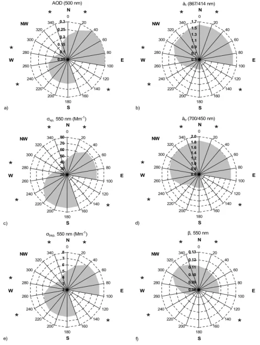
MAO station are presented in Table 2. Significant differ-ences, in most cases characteristic of the sources present in the various sectors, are found (Fig. 5). Values were not as-signed for the eastern-southeastern sector, since there were no trajectories originating from there, as already mentioned. At the borders of the sectors average values between adjacent sectors are used. A consistent distribution pattern is evident for all three extensive quantities. The minimum values of AOD, σsp and σbsp are in the NW sector, and then values
increase moving clockwise, reaching a maximum in the E sector, and then decrease again for air masses from the S and the W sectors. In contrast, minimum values of ˚aτ and ˚aσ are
found for the S sector and maxima for the N and E sectors ( ˚aσ shows only minor variability and only for the S sector
are values significantly different). Finally, β ratios have their minimum values in the S sector and maximum values in the NW sector.
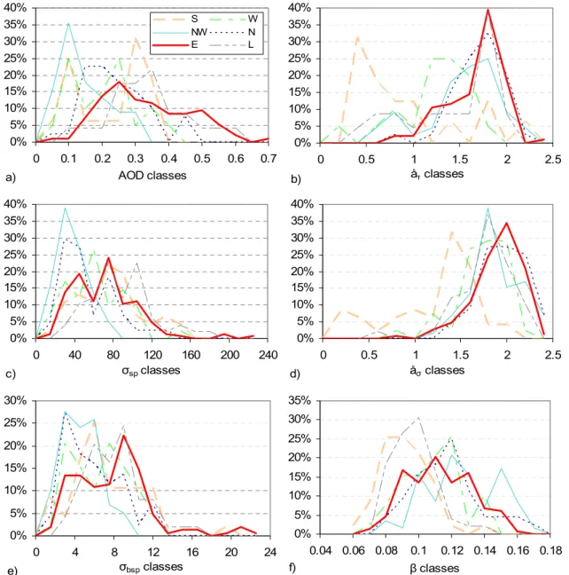
More detailed information on these spatial patterns is re-vealed by calculating the frequency distribution of aerosol optical properties for each different sector (Fig. 6). As shown in Fig. 6a, AOD values higher than 0.45 are found to origi-nate only from the E and L sector, which both have a rela-tively flat distribution, whereas a rather narrow distribution is revealed for the NW sector with a pronounced frequency peak at the 0.1–0.15 class. The distribution in the N sector represents a transition between the two most different sectors (E and NW). Finally, both the S and the W distributions ap-pear to be bi-modal, with one mode describing the lower val-ues and the other being partly shifted as one moves from the
E sector maximum to the NW minimum. From the distribu-tions in Fig. 6b one can clearly see the influence of the Sahara dust events on the size of aerosols, as revealed by the distinct peak around 0.4–0.6 found for the S sector. This maximum is less well defined for ˚aσ, probably because most of the dust
transport occurs at higher altitudes and does not influence surface aerosol properties as much as the column-integrated values (Formenti et al., 2001b; Andreae et al., 2002). The frequency distribution for ˚aτ in the W sector is shifted to
higher values serving again as a transition to the NW and N sectors, for which nearly identical and relatively broad dis-tributions with maxima near 1.7 are found. Finally, a peak at the same position is present for the E and L sectors. The nar-rower frequency peak in these sectors suggests a more con-stant particle size distribution in the air masses arriving from these sectors. The similarity between the distributions in the E and L sectors is probably due to the fact that most of the L (local) trajectories actually arrive from easterly directions and that the two sectors include common pollution sources from eastern Balkan countries (L) and former Soviet Union countries (E). The same general pattern is evident for σspand
σbsp(Figs. 6c, 6e) with minimum values originating from the
N and NW sectors, while the distributions of the rest of the sectors are not separable.
3.3 Seasonality of aerosol optical properties
The seasonal variability of aerosol optical properties is mainly related to the seasonal characteristics of the
E. Gerasopoulos et al.: Aerosol optical properties in Northern Greece 2031
Table 2. Basic statistical quantities of aerosol optical properties at MAO (daily values) sorted by the air mass sector origins. Averages are
accompanied by their standard deviation.
AOD S W NW N E L Average 0.21±0.11 0.18±0.10 0.12±0.07 0.21±0.09 0.30±0.13 0.31±0.12 Maximum 0.33 0.39 0.28 0.41 0.69 0.58 Minimum 0.05 0.05 0.03 0.05 0.05 0.08 N obs. 16 20 45 40 95 23 ˚aτ S W NW N E L Average 0.82±0.58 1.14±0.39 1.44±0.41 1.61±0.27 1.57±0.31 1.34±0.48 Maximum 2.08 1.78 2.01 2.03 2.25 1.93 Minimum 0.3 0.18 0.53 0.62 0.61 0.39 N obs. 16 20 44 40 96 23 σsp(Mm−1) S W NW N E L Average 73±40 54±29 32±16 46±26 68±42 79±32 Maximum 235 145 73 122 246 166 Minimum 10 8 8 12 15 18 N obs. 47 41 59 44 148 49 σbsp(Mm−1) S W NW N E L Average 6.3±3.3 5.8±2.9 3.9±1.9 5.1±2.8 7.1±4.0 7.3±3.0 Maximum 18.3 12 8.3 11.5 21.1 16.2 Minimum 0.8 1.1 1.1 1.3 1.1 1.8 N obs. 47 39 58 44 148 49 ˚aσ S W NW N E L Average 1.1±0.5 1.6±0.3 1.8±0.3 1.9±0.2 1.8±0.3 1.7±0.3 Maximum 1.85 2.1 2.3 2.3 2.3 2.2 Minimum 0.04 0.7 1.2 1.3 0.7 0.6 N obs. 47 41 59 44 148 49 β S W NW N E L Average 0.086±0.01 0.103±0.02 0.121±0.02 0.111±0.02 0.107±0.02 0.093±0.01 Maximum 0.14 0.13 0.16 0.16 0.16 0.14 Minimum 0.05 0.06 0.07 0.07 0.06 0.07 N obs. 47 39 58 44 148 49
production, transport and removal processes of aerosols over a specific region. In many studies (e.g. Michalsky et al., 2001; Holben et al., 2001; Alexandrov et al., 2002b) a sum-mer peak has been found for AOD, while larger aerosols dominate during winter.
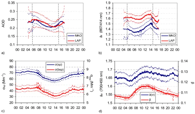
Monthly means of aerosol optical properties at MAO and LAP are presented in Fig. 7. At MAO (Fig. 7a) a distinct annual cycle is seen with clear summer maximum (August) and winter minimum (December) for AOD, ˚aτ and ˚aσ. The
second peak in October for ˚aτ can be attributed to particular
days in October 1999 and 2001 with higher values for the ˚
Angstr¨om exponents and slightly higher ones for AOD. The data show that, on a climatological basis, near background
conditions are encountered at MAO only during November and December, with AOD down to 0.1 and ˚a below 1.2 indi-cating the possible influence from sea-spray aerosols. Dur-ing summer, enhanced turbidity, the absence of wet removal processes, as well as the prevailing east sector under more stagnant meteorological conditions, result in the build-up of aerosols. The same conditions are also favorable to enhanced pollution near urban areas.
In contrast, no clear annual cycle is revealed at LAP (Fig. 7b). This can be attributed to the fact that sources of pollution with different seasonal characteristics (central heating, transportation, industrial activities etc.) are su-perimposed on the seasonality related to the change of
2032 E. Gerasopoulos et al.: Aerosol optical properties in Northern Greece
Figure 4. Sectors used for the classification of the back trajectories ending at MAO.
NW W S N E L LAP MAO
Fig. 4. Sectors used for the classification of the back trajectories
ending at MAO.
meteorological patterns. An extreme peak in August at LAP reconfirms that part of the seasonality at MAO is due to enhanced pollution, but one has still to bear in mind that the periods of measurements at the two sites are not the same (MAO: June 1999–Augugst 2000 and July 2001– March 2002, LAP: February 2001–March 2002) and August 2001 has been an exceptional month, influenced by biomass burning from areas at the northern coast of the Black Sea (Salisbury et al., 2003; Balis et al., 2003b).
The seasonal variability of σspand σbsp (Fig. 7c) is quite
different. Following a maximum in August, there is an even larger one in the fall (November), whereas a minimum is seen during spring. However, it should be mentioned that values for April, May and June are mainly from 2000 and that dur-ing this period the lowest values of the whole data set are found. The seasonal cycle of the planetary boundary layer (PBL) thickness (Balis et al., 2003a) could be responsible for the fall and winter maximum in σsp. The PBL is shallower
in fall and winter and thus aerosols are confined to a thinner layer. In contrast, ˚aσ is consistent with the seasonality in ˚aτ
since both show the same summer maximum, with the spe-cific annual cycle being much more distinct for ˚aσ. The same
pattern is also followed by β (Fig. 7d).
3.4 Diurnal variability of aerosol optical properties To investigate the diurnal variability of the aerosol optical properties, we used higher resolution data (1-min and 2-min averages of the quantities measured directly and indirectly by the two instruments). A distinct diurnal cycle is observed for all quantities, as seen in Fig. 8. AOD values decrease at both sites (Fig. 8a) around 06:00–08:00 UTC, reach a minimum at
about 12:00–14:00 UTC and then start increasing again dur-ing afternoon (12:00 UTC corresponds to 10:28 solar time at MAO). The column ˚Angstr¨om exponents, ˚aτ, (Fig. 8b) also
show a decrease in the morning, more intense at MAO than at LAP, and then they increase until 14:00 UTC, when they are subject to an abrupt decrease. Observing AOD for indi-vidual days, it is seen that there are no abrupt changes within the day and specific patterns are found. The most common patterns are those of AOD decreasing during the day and ei-ther reaching a plateau during afternoon or increasing again, but not reaching the same values as in the early morning.
The diurnal variation from the nephelometer data covers the full 24-h period, but the results indicate more or less the same behavior. Both σspand σbsp(Fig. 8c) decrease around
08:00 UTC, reach a minimum value at about 14:00 UTC and then increase until 20:00–22:00 UTC, after which they re-main on a plateau during the whole night. The pattern for ˚aσ
is similar (Fig. 8d), but shows a phase shift of about 2–3 h, with maxima and minima occurring earlier than for the other parameters. The minimum occurs at 06:00 UTC, then values rise until 12:00 UTC and then a decrease is observed during afternoon. A similar pattern is found for β with minimum and maximum preceding those of ˚aσ.
Gebhart et al. (2001) refer to five different diurnal patterns for optical properties of aerosols at various stations in the US, mainly related to the relationship between RH and scat-tering. Many of the patterns were linked to local sources or local meteorology whereas factors causing diurnal variability in particle concentration or composition are also important. At MAO and LAP, the diurnal variability of the optical prop-erties of aerosols (Fig. 8) follows the heating of the surface by the sun, suggesting that this pattern is mainly driven by the effect of relative humidity (RH) on the size and the composi-tion of aerosols. Numerous studies (H¨anel, 1976; Fitzgerald et al., 1982; Charlson et al., 1984; Horvath, 1996) have fo-cused on the change of particle size with RH for different types of atmospheric aerosols.
In order to explore the role of RH, its diurnal variabil-ity was derived using the internal RH measurements of the nephelometer. The instrument was located in a small room directly under the roof of the building, which generally was a few degrees warmer than the ambient temperature, so that internal RH was somewhat lower than that of the ambient air. As seen in Fig. 9, RH has a distinct diurnal cycle in general agreement with those of the aerosol optical properties. More specifically, regression analysis shows a strong correlation between RH with σsp and σbsp (r2=0.98 and 0.92,
respec-tively) with a time delay of 1–1.5 h and a strong anticorrela-tion with β (r2= −0.96) at zero lag. The anticorrelation with ˚aσ is weaker (r2= −0.74) possibly due to the fact that ˚aσ is
influenced by the instrumental noise on the scattering coef-ficients. The additional time delay of ˚aτ in comparison with
˚aσ can be attributed to the fact that since the heating of the
atmosphere is taking place from the surface and upwards, it takes some time to affect the relative humidity of the column
E. Gerasopoulos et al.: Aerosol optical properties in Northern Greece 2033 Figure 5. Rose diagrams of the source contribution to aerosol optical properties using air mass
trajectory analysis. Stars mark the boundaries of the defined sectors.
AOD (500 nm) 0.05 0.1 0.15 0.2 0.25 0.3 0 20 40 60 80 100 120 140 160 180 200 220 240 260 280 300 320 340 E N NW W S
*
*
*
*
*
a) åτ (867/414 nm) 0.5 0.7 0.9 1.1 1.3 1.5 1.7 0 20 40 60 80 100 120 140 160 180 200 220 240 260 280 300 320 340 E N NW W S*
*
*
*
*
b) σsp, 550 nm (Mm-1) 20 30 40 50 60 70 80 0 20 40 60 80 100 120 140 160 180 200 220 240 260 280 300 320 340 E N NW W S*
*
*
*
*
c) σbsp, 550 nm (Mm-1) 2 3 4 5 6 7 8 0 20 40 60 80 100 120 140 160 180 200 220 240 260 280 300 320 340 E N NW W S*
*
*
*
*
e) β, 550 nm 0.08 0.09 0.10 0.11 0.12 0.13 0 20 40 60 80 100 120 140 160 180 200 220 240 260 280 300 320 340 E N NW W S*
*
*
*
*
f) åσ (700/450 nm) 0.6 0.8 1.0 1.2 1.4 1.6 1.8 2.0 0 20 40 60 80 100 120 140 160 180 200 220 240 260 280 300 320 340 E N NW W S*
*
*
*
*
d)Fig. 5. Rose diagrams of the source contribution to aerosol optical properties using air mass trajectory analysis. Stars mark the boundaries
of the defined sectors.
that the MFR sees. Moreover, it should be pointed out that it is difficult to predict humidity effects in the column based on surface measurements of humidity.
But can the RH variability explain the whole of the di-urnal cycle of the optical properties? To answer this ques-tion, a correction factor f(RH) describing the hygroscopic growth of the aerosol particles with increasing RH is cal-culated, according to the equation f (RH)=a·(1−RH/100)b (Kasten, 1969; H¨anel, 1976). The choice of the constants a and b vary for different chemical composition of the aerosols (Day and Malm, 2001). Since no representative values are known for MAO, different constants (Day and Malm, 2001;
Clarke et al., 2002) were applied and σsp was corrected
ac-cording to the f (RH) (Fig. 9). Depending on the choice of the constants 45–60% of the diurnal cycle is explained by RH, but a considerable part still remains unexplained.
This part could be attributed to the contribution of local circulation systems persistent under certain meteorological conditions. Since both measuring sites (LAP and MAO) are very close to the sea, under weakening of the synoptic winds local circulation systems develop, which often lead to a sea-breeze circulation cell. This circulation pattern is stronger and appears more often during the warm period. Its presence results in a shallower PBL (e.g. Melas et al., 1998) and in
2034 E. Gerasopoulos et al.: Aerosol optical properties in Northern Greece
Figure 6. Frequency distribution of each optical property sorted by the air mass origins. Class
percentage occurrence is referred to the specific sector.
0% 5% 10% 15% 20% 25% 30% 35% 40% 0 0.1 0.2 0.3 0.4 0.5 0.6 0.7 AOD classes S W NW N E L a) 0% 5% 10% 15% 20% 25% 30% 35% 40% 0 0.5 1 1.5 2 2.5 åτ classes b) 0% 5% 10% 15% 20% 25% 30% 35% 40% 0 40 80 120 160 200 240 σsp classes c) 0% 5% 10% 15% 20% 25% 30% 0 4 8 12 16 20 24 σbsp classes e) 0% 5% 10% 15% 20% 25% 30% 35% 0.04 0.06 0.08 0.1 0.12 0.14 0.16 0.18 β classes f) 0% 5% 10% 15% 20% 25% 30% 35% 40% 0 0.5 1 1.5 2 2.5 åσ classes d)
Fig. 6. Frequency distribution of each optical property sorted by the air mass origins. Class percentage occurrence is referred to the specific
sector.
a diurnal variation of both wind speed and wind direction. In a typical sea breeze pattern it is expected that the wind speed reaches maximum values around 08:00–09:00 UTC and remain constant until the afternoon (16:00–17:00 UTC) for places that are a few kilometers inland. When the sea-breeze flow pattern is established both at the surface and up to the mixing height, the boundary-layer air originates from the sea. This pattern can introduce different aerosol sources during most of the day compared to the sources that are as-sociated with the synoptic flow over the area. The diurnal variability of the ˚Angstr¨om exponent shown in Fig. 8 indi-cates changes in the aerosol type and is in phase with the evolution of the sea-breeze cell.
Additional results are derived by sorting the diurnal vari-ability by seasons and trajectory origins. Thus, extract-ing the diurnal cycles for pairs of months (not shown here) one can see that during winter-spring (November–December, January–February and less during March–April), when the maximum diurnal range of RH is observed, the amplitude of the diurnal cycle of both σsp and σbsptakes its maximum
value as well. When sorting the diurnal variability by the tra-jectory origins it is shown that when air masses come from the S–SW sectors then the diurnal cycle of σsp and σbspis
more intense. In combination with the fact that the decrease of the values is prolonged during the afternoon, this possibly reflects the local sea breeze system.
E. Gerasopoulos et al.: Aerosol optical properties in Northern Greece 2035
Figure 7. Seasonal variation of aerosol optical properties at both stations. Error bars
corre-spond to the 95% confidence level. In Fig. 7a, empty points were calculated using the
correla-tion of optical depth and the Angström exponent between LAP and MAO because of the lack
of an adequate number of measurements at the latter site for the specific months.
0 0.1 0.2 0.3 0.4 0.5 0.6 Ja n Fe b Ma r Ap r Ma y Ju n Ju l Au g Se p Oc t No v De c AO D 0.0 0.2 0.4 0.6 0.8 1.0 1.2 1.4 1.6 1.8 2.0 å τ (8 67 /4 14 nm ) AOD å(τ) b) LAP 0 0.1 0.2 0.3 0.4 0.5 0.6 Ja n Fe b Ma r Ap r Ma y Ju n Ju l Au g Se p Oc t No v De c AO D 0.0 0.2 0.4 0.6 0.8 1.0 1.2 1.4 1.6 1.8 2.0 å τ (8 67 /4 14 nm ) AOD å(τ) a) MAO 0 10 20 30 40 50 60 70 80 90 100 Ja n Fe b Ma r Ap r May Ju n Ju l Au g Se p Oc t No v De c σ sp ( Mm -1) 2 4 6 8 10 12 14 σ bs p ( Mm -1 ) σ(sp) σ(bsp) c) MAO 1.1 1.2 1.3 1.4 1.5 1.6 1.7 1.8 1.9 2 2.1 Ja n Fe b Ma r Ap r May Ju n Ju l Au g Se p Oc t No v De c åσ (7 00/ 45 0 n m ) 0.08 0.09 0.10 0.11 0.12 0.13 0.14 0.15 β å(σ) β d) MAO
Fig. 7. Seasonal variation of aerosol optical properties at both stations. Error bars correspond to the 95% confidence level. In (a), empty
points were calculated using the correlation of optical depth and the ˚Angstr¨om exponent between LAP and MAO because of the lack of an
adequate number of measurements at the latter site for the specific months.
4 Further analysis
4.1 Comparison between rural and urban measurements – estimation of contributions from local pollution As already mentioned, the key difference between the two sites is the fact that Thessaloniki (LAP) is the main urban center of the region, and is therefore impacted by local pol-lution sources, while MAO is remote enough to be consid-ered as a rural site. On the other hand, the sites are close enough to each other so that they are influenced simultane-ously from medium- and long-range transport. This allows us to estimate the contribution of local pollution to the aerosol radiative effects at LAP, without of course disregarding the potential influence of pollution from the Thessaloniki urban region on MAO.
For the period when both sites were operating simultane-ously, AOD values at the two sites show significant covari-ance (r2=0.76 at 500 nm and 0.69 for ˚aτ), partly bearing out
the assertion above (Fig. 10). Even though not evident in Table 1 due to the use of the entire periods for both sites in-stead of their common period, AOD values over LAP were on average higher than over MAO, reflecting local pollution in Thessaloniki (values at LAP are generally above the 1:1 line). Assuming a simple additive effect of the urban
pol-lution, the mean of the AOD differences would express the contribution of the pollution, provided that clear days and days with transport from Thessaloniki to MAO are excluded. Also, one has to consider that on a climatological basis the differences in transport from remote sources at the two sites are not significant. In order to investigate the above, the dif-ferences of AOD at MAO and LAP were categorized accord-ing to the direction of the arrivaccord-ing air masses. In general, small differences (many of them not exceeding the uncer-tainty of the measurements) are found for all sectors except the Eastern one. This is a combination of the fact that some sectors (NW-N) were related to the transport of cleaner air masses (Sect. 3.2) and that in the sectors from SW to NW ur-ban pollution at Thessaloniki affects MAO. On the contrary, for air masses from the E sector, the differences become sig-nificant and more consistent. These days are more frequent during summers, when also meteorological conditions favor the trapping of pollution, and during which there is no trans-port of urban pollution to MAO.
Thus, when only the days with air masses from the E sec-tor are considered, a linear regression analysis results in a slope of 0.9±0.14 indicating that there is indeed a constant shift to higher values for LAP that could on average give an estimation of the local pollution sources at Thessaloniki.
2036 E. Gerasopoulos et al.: Aerosol optical properties in Northern Greece
Figure 8. Diurnal variability of aerosol optical properties at both stations. Averages (thick
lines) are calculated by the one-minute and two-minute time resolution of the MFR and the
nephelometer measurements, respectively. Dashed lines represent the 95% confidence level.
The vertical dashed lines in Fig. a) and b) correspond to the time before and after which the
change in the length of day with the season may have posed an effect on the pattern of the
di-urnal cycle. Time is in UTC.
0.1 0.15 0.2 0.25 0.3 0.35 00 02 04 06 08 10 12 14 16 18 20 22 00 AO D MAO LAP a) 20 30 40 50 60 70 80 90 00 02 04 06 08 10 12 14 16 18 20 22 00 σ sp (M m -1 ) 5 6 7 8 9 10 σ bs p (M m -1 ) σ(sp) σ(bsp) c) 1.5 1.55 1.6 1.65 1.7 1.75 00 02 04 06 08 10 12 14 16 18 20 22 00 å σ ( 700 /450 nm ) 0.1 0.11 0.12 0.13 0.14 β å(σ) β d) 1.1 1.2 1.3 1.4 1.5 1.6 1.7 1.8 1.9 00 02 04 06 08 10 12 14 16 18 20 22 00 å τ (867/ 414 nm ) MAO LAP b)
Fig. 8. Diurnal variability of aerosol optical properties at both stations. Averages (thick lines) are calculated by the one-minute and
two-minute time resolution of the MFR and the nephelometer measurements, respectively. Dashed lines represent the 95% confidence level. The vertical dashed lines in (a) and (b) correspond to the time before and after which the change in the length of day with the season may have posed an effect on the pattern of the diurnal cycle. Time is in UTC.
Figure 9. Diurnal variability of the internal relative humidity of the nephelometer and the scattering coefficient, σsp. Corrected σsp values according to f(RH) for four different choices
of a and b. As seen from the top: a) a=0.841, b=0.368, b) a=0.831, b=0.481, c) a=0.805, b=0.545, d) a=0.950, b=0.447. Constants for case a) were taken from Clarke et al. (2002) and for the rest of the cases they were extrapolated from data given in Day and Malm (2001).
30 35 40 45 50 55 60 65 70 00 02 04 06 08 10 12 14 16 18 20 22 00 σ sp (Mm -1 ) 35 40 45 50 55 RH σ(sp) corrected σ(sp) RH
Fig. 9. Diurnal variability of the internal relative humidity of the
nephelometer and the scattering coefficient, σsp. Corrected σsp
val-ues according to f (RH) for four different choices of a and b. As seen from the top: a) a=0.841, b=0.368, b) a=0.831, b=0.481, c) a=0.805, b=0.545, d) a=0.950, b=0.447. Constants for case a) were taken from Clarke et al. (2002) and for the rest of the cases they were extrapolated from data given in Day and Malm (2001).
This contribution is acquired from the intercept, 0.19±0.05 at 500 nm, leading to a contribution of 35±10% for the aver-age AOD over LAP. For the rest of the cases the contribution, calculated from the mean of the AOD differences at the two sites, varies between 3–10%.
4.2 Estimation of aerosol scale height
The aerosol scale height, which is commonly used as the equivalent depth of the optically active aerosol layer of the atmosphere at an assumed constant pressure equal to the sur-face pressure, can be estimated by combining the extinction coefficient, σep, and the AOD at MAO (e.g. Formenti et al.,
2001b). In general, if a linear relationship between the two parameters exists (AOD=H∗σep+b), then the slope of the
regression line gives the aerosol scale height, under the as-sumption that aerosol concentration is constant with height within the lower part of the atmosphere, near the ground and up to the height, H . The variance explained by the regres-sion gives an indication of how well the column extinction is represented by a measurement at the bottom of the boundary layer. The intercept, on the other hand, represents more or less constant contributions to extinction by free tropospheric and stratospheric background aerosols.
However, for the calculation of σep apart from σsp the
aerosol absorption coefficient, σabs, is also needed. Shettle
and Fenn (1979) provide the single scattering albedo, ω, for various types of aerosols, ranging from 0.7 (urban) to 0.98 (maritime) with ω equal to 0.94 and 0.96 for rural and tropo-spheric background, respectively. Moreover, estimations of ωover the Eastern Mediterranean show mean values within the range of 0.85–0.90 (Kouvarakis et al., 2002; Lelieveld et
E. Gerasopoulos et al.: Aerosol optical properties in Northern Greece 2037 Figure 10. Scatter plot of aerosol optical depth over LAP versus MAO for the investigation of
local pollution contribution. The dashed line represents the 1:1line. Points denoted by dia-monds express days with enhanced contribution of local pollution. The solid line indicates the average excess of optical depth measured over the urban station (LAP) and dotted lines corre-spond to the standard error of the estimation.
0 0.1 0.2 0.3 0.4 0.5 0.6 0.7 0.8 0 0.1 0.2 0.3 0.4 0.5 0.6 0.7 0.8 Rural AOD (ΜΑΟ) U rba n A O D ( LA P ) y = 0.91x + 0.19
Fig. 10. Scatter plot of aerosol optical depth over LAP versus MAO
for the investigation of local pollution contribution. The dashed line represents the 1:1line. Points denoted by diamonds express days with enhanced contribution of local pollution. The solid line indi-cates the average excess of optical depth measured over the urban station (LAP) and dotted lines correspond to the standard error of the estimation.
al., 2002; Formenti et al., 2002a, 2002b). Thus, assuming the general case of moderately absorbing aerosols (ω=0.9), σep would be 10% higher than σsp, which leads to a
cor-responding 10% reduction to the calculated aerosol scale height. Nevertheless, for the regressions below, σsp will be
used instead of σep since an exact value for ω is not
avail-able, and it must be kept in mind that the corrected value for H is H /(2−ω). Application of the correction for (ω=0.9) will also be provided.
Apart from this correction, humidity effects on neph-elometer observations should be considered. In particular, particles are drier in the nephelometer than outside and they are also drier at the surface than at higher levels in the mixed layer. This may cause a decrease in the scattering coefficients which is difficult to quantify with the available data. Thus, the estimated value for H should be considered as the upper limit of aerosol scale height.
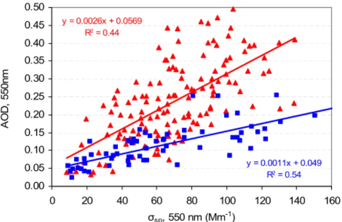
In the scatter plot between σsp and AOD at 550 nm for
the whole period (Fig. 11) a great dispersion of values can be seen, thus not fully satisfying the assumption of linear-ity for the determination of H (AOD at 550 was derived by ˚Angstr¨om’s power law approximation, τ (λ)=βλ−˚a, after constants α, β, were calculated). Nonetheless, the regression for the whole of the available data yielded a mean aerosol scale height of 2.1±0.2 km (1.9±0.18 km, for ω=0.9). When we stratified the data seasonally, the aerosol scale height was found to be 1.1±0.13 km (0.96±0.11 km, for ω=0.9) during the colder period (October–March) with 54% of AOD vari-ance explained by the variability of the near-surface aerosols, whereas, during the warmer months, (April–September) H went up to 2.6±0.25 km (2.3±0.22 km, for ω=0.9). The greater scatter of the values during the warm season reflects
Figure 11. Scatter plot of aerosol optical depth, AOD, (550 nm) versus scattering coefficient,
σsp, (550 nm) for the estimation of aerosol scale height. Red triangles and blue squares denote
summer and winter data, respectively, whereas the solid lines correspond to the regression line of each group.
y = 0.0026x + 0.0569 R2 = 0.44 y = 0.0011x + 0.049 R2 = 0.54 0.00 0.05 0.10 0.15 0.20 0.25 0.30 0.35 0.40 0.45 0.50 0 20 40 60 80 100 120 140 160 σsp, 550 nm (Mm-1) A O D , 55 0n m
Fig. 11. Scatter plot of aerosol optical depth, AOD, (550 nm)
ver-sus scattering coefficient, σ|chemsp, (550 nm) for the estimation of
aerosol scale height. Red triangles and blue squares denote summer and winter data, respectively, whereas the solid lines correspond to the regression line of each group.
the more variable aerosol loading and the greater fluctuation of the boundary layer thickness.
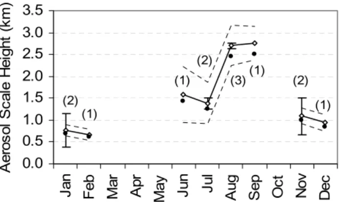
We also calculated the aerosol scale height for those in-dividual months when data coverage was sufficient for both AOD and σsp. As seen in Fig. 12, a distinct seasonality with
a peak of 2.7 km (2.5 km, for ω=0.9) in August–September (coinciding with the peak in AOD seasonal cycle) is seen, whereas during the cold months (November–February) H is between 0.5–1 km. The corrected heights remain well within the standard error of the estimations. The seasonal cycle of the aerosol scale height relates to the seasonal change in the boundary layer thickness as shown by individual estimations of the PBL by LIDAR and radiosondes at Thessaloniki. More specifically, the PBL during 2001 varied between 0.3–0.5 km during winter, whereas for summer it had values about 1.5– 1.7 km, exceeding 2 km under certain circumstances (Balis et al., 2003a). This result is consistent with the assump-tion that most of the aerosols are present within the boundary layer, and that there is a lesser contribution to scattering from free tropospheric aerosols. This is additionally supported by the relatively small value of the regression intercept (0.0490– 0.057 for optical depth at 550 nm), indicating an average con-tribution of 24–28% of the total AOD from aerosols outside of the boundary layer, part of which can be attributed to the transport of dust from the Sahara desert.
5 Conclusions
Aerosol optical properties from two sites in Northern Greece, the first at Thessaloniki (LAP), the main city of the region, and the second at Ouranoupolis (MAO), 100 km to the east, have been analyzed in order to provide information about the climatological characteristics of aerosol optical proper-ties. The data cover a time span of 3 years.
2038 E. Gerasopoulos et al.: Aerosol optical properties in Northern Greece
Figure 12. Seasonal variation of the estimated aerosol scale height. Dashed lines represent the
standard error of the height estimation. Numbers in brackets express the number of years from
which monthly estimates of H were derived. Error bars correspond to the standard deviation
when months from different years are available. Black dots represent the reduction to the
scale height when absorption is taken under consideration for single scattering albedo of 0.9.
0.0 0.5 1.0 1.5 2.0 2.5 3.0 3.5 Ja n Fe b Ma r Ap r Ma y Ju n Ju l Au g Se p Oc t No v De c A er os ol S cal e H ei gh t ( km ) (1) (1) (1) (1) (2) (2) (2) (3)
Fig. 12. Seasonal variation of the estimated aerosol scale height.
Dashed lines represent the standard error of the height estima-tion. Numbers in brackets express the number of years from which monthly estimates of H were derived. Error bars correspond to the standard deviation when months from different years are available. Black dots represent the reduction to the scale height when absorp-tion is taken under consideraabsorp-tion for single scattering albedo of 0.9.
The mean value of 0.23 for AOD at 500 nm at both sites is well within the range of values observed previously in the area (Formenti et al., 2001a; 2001b). Pinker et al. (1997) has given a range of 0.135–0.334 for monthly means of the AOD at the Negev desert (Israel) over a seven year period (1985–1992), whereas long term observations of AOD at var-ious areas in the US can be found in Michalsky et al. (2001) and Alexandrov et al. (2002b). During summer, AOD val-ues increase considerably, remaining persistently between 0.3 and 0.5, while during specific cases they go up to 0.7– 0.8. A value of 0.26 for AOD from satellite retrieval for the eastern Mediterranean during summer is given by Husar et al. (1997). The higher values of AOD are mainly associated with fine aerosols as indicated by the ˚aτexponents. At MAO,
a mean value of 65±40 Mm−1 for σsp at 550 nm reflects
the impact of continental pollution on the region. During the colder months values are usually well above 100 Mm−1, reaching even 250 Mm−1under certain circumstances. The level of σspis well above the limits of 10–30 Mm−1reported
for unpolluted marine air (Formenti et al., 2001 and refer-ences therein). This limit is exceeded during 80% of the days for which measurements were available, and for 50% of the days values are above the mean value of 57 Mm−1
given by Seinfeld and Pandis (1998) for the average conti-nental background. The frequency distributions of AOD, σsp
and σbsp have revealed the existence of different modes of
aerosol loading associated with background conditions, av-erage continental aerosol concentrations, and highly polluted air masses from either local and regional sources or from longer range transport.
The investigation of source regions via air mass trajec-tory analysis has shown that enhanced AOD, σsp and σbsp
are found for the E sector. Observations of enhanced SO2
over Southeastern Europe by GOME (Eisinger and Burrows,
1998) as well as the fact that during NE directions about 70% of the SO2column can be attributed to lignite combustion in
power plants in Bulgaria and Romania (Zerefos et al., 2000), can help to explain the maxima in aerosol loadings from the easterly sector. Biomass burning from areas at the northern coast of the Black Sea (Salisbury et al., 2003; Balis et al., 2003b) may also contribute episodically. Cleaner conditions, associated with fine aerosol particles, are found for the NW direction, in spite of the presence of the most industrialized countries of Central Europe being in this sector. The reason for this could be the meteorological conditions during which NW air mass trajectories reach Northern Greece, namely in-creased wind speed and atmospheric washout, and the fact that this path is often associated with subsidence from the upper troposphere (Gerasopoulos et al., 2001). The influence of Sahara dust events is clearly shown by both ˚a exponents and backscatter ratio β. The values of ˚aτ for the S sector
(Fig. 6b) are distributed around 0.4, which is typical of min-eral dust (Kaufman, 1993), while the corresponding ˚aσ
expo-nents from scattering are shifted to higher values, since dust layers are present mainly at elevated altitudes. The coarse dust particles are also responsible for the enhanced scatter-ing for the S sector.
The temporal variability of aerosol optical properties at two time scales was also investigated. A distinct summer maximum was revealed for AOD and ˚aτ at MAO, but the
seasonality at LAP was masked by the seasonal variability of local pollution sources. Only during November and Decem-ber can near background conditions be observed at MAO, with AOD down to 0.1 and ˚a exponents below 1.2 indicating the possible influence from sea-spray aerosols. The season-ality is mainly driven by the fact that during summer 50% of the trajectories (for the days that measurements were avail-able) came from the E sector. This fact, in combination with enhanced turbidity, the absence of wet removal processes and conditions favorable to enhanced pollution, leads to the build-up of aerosols during summer. A diurnal cycle of all properties was evident. In the morning, AOD, σspand σbsp
decrease simultaneously with humidity and reach a minimum at mid-day. About 45–60% of the diurnal cycle amplitude was explained by the effect of humidity on the size of hygro-scopic aerosols. The rest of the variability was attributed to the local sea breeze system that results in a shallower PBL and in a diurnal variation of both wind speed and wind di-rection, thus introducing different aerosol sources than those resulting from the synoptic flow over the area.
From the days with higher values at LAP than at MAO an estimation of the contribution of the local pollution sources to Thessaloniki’s AOD was attempted. During summer, when the effect of urban pollution is favored by meteoro-logical conditions, a constant shift by 0.19±0.05 at 500 nm was found, leading to a contribution of 35±10% for the av-erage AOD over LAP, while in general it ranges between 3– 10%. Finally, the equivalent thickness of the optically active aerosol layer (aerosol scale height) was found to be related
E. Gerasopoulos et al.: Aerosol optical properties in Northern Greece 2039 to the height of the boundary layer, with values between 0.5–
1 km during winter and up to 2.5–3 km during summer.
Acknowledgements. This research was financially supported by the Max Planck Society, Germany.
References
Alexandrov, M. D., Lacis, A. A., Carlson, B. E., and Cairns, B.: Re-mote sensing of atmospheric aerosols and trace gases by means of Multifilter Rotating Shadowband Radiometer, Part I: Retrieval algorithm, J. Atmos. Sci., 59, 524–543, 2002a.
Alexandrov, M. D., Lacis, A. A., Carlson, B. E., and Cairns, B.: Re-mote sensing of atmospheric aerosols and trace gases by means of Multifilter Rotating Shadowband Radiometer, Part II: Clima-tological Applications, J. Atmos. Sci., 59, 544–566, 2002b. Anderson, T. L. and Ogren, J. A.: Determining aerosol radiative
properties using the TSI 3563 integrating nephelometer, Aerosol Sci. Tech., 29, 57–69, 1998.
Andreae, M. O.: Climatic effects of changing atmospheric aerosol levels, in World Survey Climatology, Future Climates of the world, edited by Henderson-Sellers, A., 16, 341–392, Elsevier, Amsterdam, 1995.
Andreae, T. W., Andreae, M. O., Ichoku, C., Maenhaut, W.,
Cafmeyer, J., Karnieli, A., and Orlovsky, L.: Light
scat-tering by dust and anthropogenic aerosol at a remote site in the Negev desert, Israel, J. Geophys. Res., 107, 4008, doi:10.1029/2001JD900252, 2002.
˚
Angstr¨om, A.: On the transmission of sun radiation and on dust in the air, Geogr. Ann., 2, 156–166, 1929.
Bais, A., Zerefos, C. S., and McElroy, C. T.: Solar UV-B measure-ments with the double-and-single monochromator Brewer ozone spectrophotometers, Geophys. Res. Let., 23, 8, 833–836, 1996. Balis, D. S., Zerefos, C. S., Kourtidis, K., Bais, A. F., Hofzumahaus,
A., Kraus, A., Schmitt, R., Blumthaler, M., and Gobbi, G. P.: Measurements and modeling of photolysis rates during the PAUR II campaign, J. Geophys. Res., 10.1029/2000JD000136, 2002. Balis, D.S, Amiridis, V., Zerefos, C., and Melas, D.: Seasonal
vari-ability of the mixed layer height using radiosonde and lidar mea-surements, in preparation, 2003a.
Balis D.S, Amiridis, V., Zerefos, C., Gerasopoulos, E., Andreae, M.O., Zanis, P., Kazantzidis, A., Kazantzis, S., and Papayannis, A.: Raman lidar and sunphotometric measurements of aerosol optical properties over Thessaloniki, Greece during a biomass burning episode, Atmos. Environ., 37, 32, 4529–4538, 2003b. Balis D., Amiridis V., Zerefos C., Gerasopoulos E., and Andreae
M.: Regional and long-range transported aerosols detected with a Raman lidar and filter radiometer measurements, ICAG confer-ence, EARLINET symposium, Hamburg, 11–12 February 2003. Boucher, O. and Anderson, T. L.: GCM assessment of the sensitiv-ity of direct climate forcing by anthropogenic sulphate aerosols to aerosol size and chemistry, J. Geophys. Res., 100, 26 117– 26 134, 1995.
Bruegge, C. J., Halthore, R. N., Markham, B., Spanner, M., and Wrigley, R.: Aerosol optical depth retrievals over the Konza Prairie, J. Geophys. Res., 97, 18 743–18 758, 1992.
Coakley, J. A., Cess, Jr. R. D., and Yurevich, J. B.: The effect of tropospheric aerosols on the earth’s radiation budget: A
param-eterization of for climate models, J. Atmos. Sci., 40, 116–138, 1983.
Charlson, R. J., Covert, D. S., and Larson, T. V.: Observation of the effect of humidity on light scattering by aerosols, in Hygroscopic Aerosols, edited by Rukube, T. H. and Deepak, A., 35–44, A. Deepak, Hampton, Va., 1984.
Charlson, R. J., Langner, J., Rodhe, H., Leovy, C. B., and Warren, S. G.: Perturbation of the northern hemisphere radiative balance by scattering from anthropogenic sulphate aerosols, Tellus A, 43, 152–163, 1991.
Clarke, A. D., Howell, S., Quinn, P. K., Bates, T. S., Ogren, J. A., Andrews, E., Jefferson, A., Massling, A., Mayol-Bracero, O., Maring, H., Savoie, D., and Cass, G.: INDOEX aerosol: A comparison and summary of chemical, microphysical, and opti-cal properties observed from land, ship, and aircraft, J. Geophys. Res., 107, 8033, doi:10.1029/2001JD000572., 2002.
Day, D. E. and Malm, W. C.: Aerosol light scattering measure-ments as a function of relative humidity: a comparison between measurements made at three different sites, Atmos. Environ., 35, 5169–5176, 2001.
Eisinger, M. and Burrows, J. P.: Tropospheric Sulfur Dioxide ob-served by the ERS-2 GOME Instrument, Geophys. Res. Let., 25, 4177–4180, 1998.
Fitzgerald, J. W., Hoppel, W. A., and Vietti, M. A.: The size and scattering coefficient of urban aerosol particles at Washington D.C. as a function of relative humidity, J. Atmos. Sci., 39, 1838– 1852, 1982.
Formenti, P., Andreae, M. O., Andreae, T. W., Ichoku, C., Schebeske, G., Kettle, J., Maenhaut, W., Cafmeyer, J., Ptasin-sky, J., Karnieli, A., and Lelieveld, J.: Physical and chemical characteristics of aerosols over the Negev Desert (Israel) during summer 1996, J. Geophys. Res., 106, 4871–4890, 2001a Formenti, P., Andreae, M. O., Andreae, T. W., Galani, E., Vasaras,
A., Zerefos, C., Amiridis, V., Orlovsky, L., Karnieli, A., Wendisch, M., Wex, H., Holben, B. N., Maenhaut, W., and Lelieveld, J.: Aerosol optical properties and large scale trans-port of air masses: Observations at a coastal and a semiarid site in the eastern Mediterranean during summer 1998, J. Geophys. Res., 106, 9807–9826, 2001b.
Formenti, P., Reiner, O., Sprung, D., Andreae, M. O., Wendisch, M., Wex, H., Kindred, D., Dewey, K., Kent, J., Tzortziou,
M., Vasaras, A., and Zerefos, C.: The STAAARTE-MED
1998 summer airborne measurements over the Aegean Sea: 1. Aerosol particles and trace gases, J. Geophys. Res., 107, 4450, doi:10.1029/2001JD001337, 2002a.
Formenti, P., Boucher, O., Reiner, T., Sprung, D., Andreae, M. O., Wendisch, M., Wex, H., Kindred, D., Tzortziou, M., Vasaras, A., and Zerefos, C.: The STAAARTE-MED 1998 summer air-borne measurements over the Aegean Sea: 2. Aerosol scattering and absorption, and radiative calculations, J. Geophys. Res., 107, 4451, doi:10.1029/2001JD001536, 2002b.
Gebhart, K. A., Copeland, S., and Malm, W. C.: Diurnal and sea-sonal patterns in light scattering, extinction and relative humidity, Atmos. Environ., 35, 5177–5191, 2001.
Gerasopoulos E., Zanis, P., Stohl, A., Zerefos, C. S., Papastefanou, C., Ringer, W., Tobler, L., Huebener, S., Kanter, H. J., Tositti, L.,
and Sandrini, S.: A climatology of7Be at four high-altitude
sta-tions at the Alps and the Northern Apennines, Atmos. Environ., 35, 6347–6360, 2001.