HAL Id: hal-03162012
https://hal.archives-ouvertes.fr/hal-03162012
Submitted on 8 Mar 2021
HAL is a multi-disciplinary open access
archive for the deposit and dissemination of
sci-entific research documents, whether they are
pub-lished or not. The documents may come from
teaching and research institutions in France or
L’archive ouverte pluridisciplinaire HAL, est
destinée au dépôt et à la diffusion de documents
scientifiques de niveau recherche, publiés ou non,
émanant des établissements d’enseignement et de
recherche français ou étrangers, des laboratoires
2D Wasserstein Loss for Robust Facial Landmark
Detection
Yongzhe Yan, Stefan Duffner, Priyanka Phutane, Anthony Berthelier,
Christophe Blanc, Christophe Garcia, Thierry Chateau
To cite this version:
Yongzhe Yan, Stefan Duffner, Priyanka Phutane, Anthony Berthelier, Christophe Blanc, et al.. 2D
Wasserstein Loss for Robust Facial Landmark Detection. Pattern Recognition, Elsevier, In press.
�hal-03162012�
2D Wasserstein Loss for Robust Facial Landmark
Detection
Yongzhe YANa,∗, Stefan DUFFNERb, Priyanka PHUTANEa, Anthony BERTHELIERa, Christophe BLANCa, Christophe GARCIAb, Thierry
CHATEAUa
aUniversit´e Clermont Auvergne, CNRS, SIGMA, Institut Pascal, Clermont-Ferrand, France bUniversit´e de Lyon, CNRS, INSA-Lyon, LIRIS, UMR5205, France
Abstract
The recent performance of facial landmark detection has been significantly im-proved by using deep Convolutional Neural Networks (CNNs), especially the Heatmap Regression Models (HRMs). Although their performance on common benchmark datasets has reached a high level, the robustness of these models still remains a challenging problem in the practical use under noisy conditions of realistic environments. Contrary to most existing work focusing on the de-sign of new models, we argue that improving the robustness requires rethinking many other aspects, including the use of datasets, the format of landmark an-notation, the evaluation metric as well as the training and detection algorithm itself. In this paper, we propose a novel method for robust facial landmark detection, using a loss function based on the 2D Wasserstein distance combined with a new landmark coordinate sampling relying on the barycenter of the indi-vidual probability distributions. Our method can be plugged-and-play on most state-of-the-art HRMs with neither additional complexity nor structural modi-fications of the models. Further, with the large performance increase, we found that current evaluation metrics can no longer fully reflect the robustness of these
∗Corresponding author
Email addresses: [email protected] (Yongzhe YAN),
[email protected] (Stefan DUFFNER), [email protected] (Priyanka PHUTANE), [email protected] (Anthony BERTHELIER),
[email protected] (Christophe BLANC), [email protected] (Christophe GARCIA), [email protected] (Thierry CHATEAU)
models. Therefore, we propose several improvements to the standard evalua-tion protocol. Extensive experimental results on both tradievalua-tional evaluaevalua-tion metrics and our evaluation metrics demonstrate that our approach significantly improves the robustness of state-of-the-art facial landmark detection models. Keywords: Facial Landmark Detection, Face Alignment, Heatmap Regression, Wasserstein Distance
1. Introduction
Facial landmark detection has been a highly active research topic in the last decade and plays an important role in most face image analysis applications e.g. face recognition, face editing and face 3D reconstructions, etc.. Recently, neural network-based Heatmap Regression Models (HRMs) outperform other methods
5
due to their strong capability of handling large pose variations. Unlike Coordi-nate Regression CNNs which directly estimate the numerical coordiCoordi-nates using fully-connected layers at the output, HRMs usually adopt a fully-convolutional CNN structure. The training targets of HRMs are heatmaps composed of Gaus-sian distributions centered at the ground truth position of each landmark [1].
10
Recently, HRMs have brought the performance on current benchmarks to a very high level. However, maintaining robustness is still challenging in the practi-cal use, especially with video streams that involve motion blur, self-occlusions, changing lighting conditions, etc.
We think that the use of geometric information is the key to further improve
15
the robustness. As faces are 3D objects bound to some physical constraints, there exists a natural correlation between landmark positions in the 2D images. This correlation contains important but implicit geometric information. How-ever, the L2 loss that is comonly used to train state-of-the-art HRMs is not able to exploit this geometric information. Hence, we propose a new loss function
20
based on the 2D Wasserstein distance (loss).
The Wasserstein distance, a.k.a. Earth Mover’s Distance, is a widely used metric in Optimal Transport Theory [2]. It measures the distance between two
Activation Difference
Geometry Difference
Ground truth Distribution
Predicted Distribution
Figure 1: An illustration of the Wasserstein loss between two 1D distributions. Standard L2 loss only considers the “activation” difference (point-wise value difference, vertical gray arrows), whereas the Wasserstein loss takes into account both the activation and the geometry differences (distance between points, horizontal blue arrow).
probability distributions and has an intuitive interpretation. If we consider each probability distribution as a pile of earth, this distance represents the minimum
25
effort to move the earth from one pile to the other. Unlike other measurements such as L2, Kullback-Leibler divergence and Jensen-Shannon divergence, the most appealing property of the Wasserstein distance is its sensitivity to the geometry (see Fig. 1).
The contribution of this article is two-fold:
30
• We propose a novel method based on the Wasserstein loss to significantly improve the robustness of facial landmark detection.
• We propose several modifications to the current evaluation metrics to re-flect the robustness of the state-of-the-art methods more effectively.
2. Related work
35
2.1. Heatmap Regresion Models (HRMs)
Recently, HRMs have superseded other facial landmark detection methods with the advent of very powerful deep neural network models. Bulat et al. [3, 4] proposed to use the stacked Hourglass Model [5] for facial landmark detection. Their method is now widely used in lots of face related applications.
To improve the accuracy, Wu et al. [6] proposed to predict the boundary of the face and facial components on the heatmap rather than a Gaussian distribu-tion of a landmark, which increases the model sensitivity to the boundary. Liu et al. [7] also proposed a method to improve accuracy of the detection by search-ing the real ground truth position along the boundary. Compared to learnsearch-ing
45
the boundary explicitly, Dapogny et al. [8] proposed to integrate landmark-wise attention maps with a cascaded heatmap regression model. The attention map resembles the boundary map. Their method is able to learn the boundary in an end-to-end manner without explicitly training the boundary as a target. Re-cently, HRNet [9] superseded most of the state-of-the-art methods by addressing
50
the importance of the high-resolution heatmap for accuracy.
Deng et al. [10] proposed a joint multi-view HRM to estimate both semi-frontal and profile facial landmarks. Tang et al. [11] proposed quantized densely-connected U-Nets to significantly accelerate the inference of the heatmap regres-sion models. In their network, not only the parameters but also the gradients
55
are quantized.
2.2. Robust facial landmark detection
Robust facial landmark detection in images is a long-standing research topic. Numerous works [12, 13, 14, 15, 16, 17, 17, 18, 19, 20, 21, 22] propose methods to improve the overall detection robustness on Active Appearance Models [23],
60
Constrained Local Models (CLM) [24], Exemplars-based Models [25] and Cas-caded Regression Models [26]. For Coordinate Regression CNNs, Lee et al. [27] improved the robustness by using a geometric prior-generative adversarial net-work, which estimates a segmentation-like geometric map.
Specifically, the heatmap used in HRMs is conceptually connected to the
65
response map used in CLMs in terms of local activation. Both RLMS [28] and DRMF [13] made effort to alleviate the robustness problem in CLM models.
To ensure the robustness of HRMs, many researchers focus on the represen-tation of the heatmaps. Merget et al. [29] proposed a fully-convolutional local-global context network, which introduces a more local-global context in the heatmap
regression model. One advantage of this method is that this method does not re-quire face detection as a pre-precessing step. Two approaches [30, 31] concerned the uncertainty on the Gaussian distribution of each landmark. Wang et al. [31] proposed a novel Weighted Loss Map, which assigns high attentions on the pixels around the center of the Gaussian distribution. It helps the training process to
75
be more focused on the pixels that are crucial to landmark localization. Chen et al. [30] introduced the Kernel Density Deep Neural Network that produces tar-get probability map, without assuming a specific parametric distribution such as Gaussian distribution. Zou et al. [32] concerned the structural information in the heatmap regression models. To obtain robust landmark prediction, they
80
proposed to add a structural constraint based on Hierarchical Structured Land-mark Ensemble. Recently, in order to ensure the robustness for downstream tasks, Kumar et al. [33] proposed to estimate the uncertainty and the visibility of the landmarks given by the HRMs. Wan et al. [34, 35] integrated multi-order cross information into the HRM to model facial geometric constraints. Park
85
et al. [36] used spatial attention mechanism to reject impeditive local features caused by the occlusion.
Several works have been proposed for robust facial landmark detection [37, 38, 39, 40, 31] by carefully designing CNN models, by balancing the data distribution and other specific techniques. Dong et al. [41] proposed a
style-90
aggregated face generation module coupled with a heatmap regression model to predict robust results on large variance of image styles. The key idea is to develop an unsupervised data augmentation methods, which is able to apply distinct style (including gray scale/color, light/dark, intense/dull etc.) change on the training images. Zhang et al. [42] proposed a global constraint network
95
for refining the detection based on offset estimation. Chen et al. [43] combined Conditional Random Field with the CNNs to produce structured probabilistic prediction. Zou et al. [44] concerned the robustness problem with diverse crop-ping manners (related to face detection). They proposed an approach to handle the out-of-bounds landmarks and achieve transformation-invariant detection.
100
(a) Good Detection(b) Pose+Occlusion (c) Occlusion (d) Pose+Light (e) Blur (f) Blur
Figure 2: Examples of HRNet detection on 300VW-S3.
each landmark is reliable.
For video sequence, FAB [46] introduced Structure-aware Deblurring to en-hance the robustness against motion blurs. Zhu et al. [47] proposed a spatial-temporal deformable network to achieve shape-informative and robust feature
105
representation.
3. Motivation
3.1. Robustness problem of HRMs
Figure 2 shows some example results of the state-of-the-art method HR-Net [9]. HRHR-Net can handle most of the challenging situations (e.g. Fig. 2 (a)).
110
However, we observed that a well-trained HRNet still has difficulties in the prac-tical use when facing extreme poses (Fig. 2 (b)(d)), heavy occlusions (Fig. 2 (b)(c)) and motion blur (Fig. 2 (e)(f)).
These observed robustness issues are rather specific to HRMs. When us-ing Cascaded Regression Models or Coordinate Regression CNNs, even if the
115
prediction is poor, the output still forms a plausible shape. On the contrary, with HRMs, there may be only one or several landmarks that are not robustly detected whereas the others are. In addition, they may be located at completely unreasonable positions according to the general morphology of the face.
This is a well-known problem. Tai et al. [48] proposed to improve the
robust-120
ness by enforcing some temporal consistency. And the approach of Liu et al. [7] tries to correct the outliers by integrating a Coordinate Regression CNN at the end. Recently, Zou et al. [32] introduced Hierarchical Structured Landmark
En-semble to impose additional structural constraints on HRMs. In these methods, the constraints are imposed in a post-processing step, which is not integrated
125
into the HRM itself. Therefore, all these methods either add complexity to the models or require learning on a video stream.
We propose to use Waserstein loss to regularize the output of HRMs. Com-pared to aforementioned methods, our approach is more general by imposing additional geometric and global contextual constraints into the loss function.
130
This adds no complexity during inference and can be trained on both image and video datasets. With exactly the same model structure, our models can effortlessly substitute the existing ones. Besides that, we found that smoother heatmap and proper landmark sampling method also help to improve the model robustness.
135
3.2. Problem of current evaluation metrics for robustness
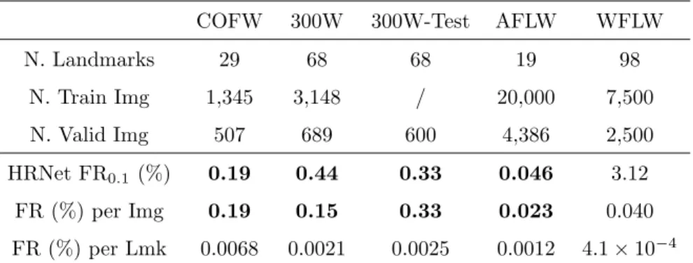
The most common metric for robustness is Failure Rate (FR). It measures the proportion of images in a (validation) set whose error is greater than a threshold. Table 1 shows the FR with an error threshold of 0.1 (FR0.1) of
HRNet. We find that this widely used FR0.1 measure is almost “saturated” on
140
several benchmarks such as COFW [12], 300W [49], 300W-Test and AFLW [50]. That is, there are only 1 , 3 , 1 and 2 failure images respectively (bold numbers in Tab. 1). This means that there are only very few challenging images for the state-of-the-art model HRNet in these datasets. At this level, this indicator is saturated and becomes difficult to interpret when comparing the robustness of
145
different methods as it is sensitive to random statistical variations. Therefore, it becomes necessary to modifiy the current evaluation metrics on these datasets and to find more challenging evaluation protocols to further decrease the gap with real-world application settings.
COFW 300W 300W-Test AFLW WFLW N. Landmarks 29 68 68 19 98 N. Train Img 1,345 3,148 / 20,000 7,500 N. Valid Img 507 689 600 4,386 2,500 HRNet FR0.1 (%) 0.19 0.44 0.33 0.046 3.12 FR (%) per Img 0.19 0.15 0.33 0.023 0.040 FR (%) per Lmk 0.0068 0.0021 0.0025 0.0012 4.1 × 10⁻⁴
Table 1: Numerical details of the facial landmark datasets and the Failure Rate (FR) of HRNet on each dataset.
4. Proposed evaluation metrics
150
4.1. Dataset
The dataset is crucial to evaluate the robustness of the model. The most common robustness issues treated in the literature concern partial occlusions and large pose variations. COFW [12] is one of the first datasets that aims at benchmarking the performance of facial landmark detection under partial
oc-155
clusion. 300W [49] comprises a challenging validation subset with face images with large head pose variations, heavy occlusion, low resolution and complex lighting conditions. AFLW [50] is a large-scale dataset including face images in extreme poses. WFLW [6] is a recently released dataset with even more chal-lenging images. All the images are annotated in a dense format (98 points). The
160
validation set of WFLW is further divided into 6 subsets based on the different difficulties such as occlusion, large pose or extreme expressions. 300VW [51] is a video dataset annotated in the same format as 300W. The validation dataset is split into three scenarios, where the third one (300VW-S3) contains the videos in highly challenging conditions.
165
4.2. Current evaluation metrics
The main performance indicator for facial landmark detection is the Nor-malised Mean Error: NME = 1
N
P
validation set, where for one image i the error is averaged over all M landmarks: NMEi= 1 M X j NMEi,j, (1)
and for each landmark j:
NMEi,j = Si,j− S ∗ i,j 2 di , (2)
where Si,j, S∗i,j∈ R
2 denote the j-th predicted and the ground truth landmarks
respectively. For each image, we consider the inter-occular distance as normal-isation distance di for 300W, 300VW, COFW, WFLW and the face bounding
box width for AFLW.
170
As mentioned before, Failure Rate FRθ measures the proportion of the
im-ages in the validation set whose NMEi is greater than a threshold θ. We will
denote this classical failure rate: FRI in the following. In the literature, FRI0.1
and FRI0.08 are the principle metrics to measure the prediction robustness as
they focus on rather large errors (i.e. 8%/10% of the normalisation distance).
175
It is also very common to compute the FRI
θ over the entire range of θ,
called the Cumulative Error Distribution (CED), which gives an overall idea on the distribution of errors over a given dataset. Finally, for easier quantitative comparison of the performance of different models, the total area under the CED distribution can be computed, which is usually denoted as the Area Under Curve
180
(AUC).
4.3. Proposed modifications to the current evaluation metric We propose three modifications to these measures:
Landmark-wise FR: Instead of computing the average failure rate per im-age: FRI, we propose to compute this measure per landmark. That is, for each
185
landmark j, the proportion of NMEi,j larger than a threshold is determined.
Finally, an average over all landmarks is computed, called FRL in the follow-ing. There are two advantages of computing the failure rate in this way: (1) With HRMs, it happens that only one or few landmarks are not well detected
(outliers). However, the FRI (per image) may still be small because the rest
190
of the landmarks are predicted with high precision and an average is computed per image. Thus, possible robustness problems of some individual landmarks are not revealed by the FRI measure. (2) FRL can provide a finer
granular-ity for model comparison, which is notably beneficial when the state-of-the-art methods have an FRI that is very close and almost zero on several benchmark
195
datasets (see FR (%) per Image/Landmark in Tab. 1).
Cross-dataset validation: Leveraging several datasets simultaneously is not new and has already been adopted by some previous works [52, 53, 54, 55, 6, 56]. Most of them focus on unifying the different semantic meanings among different annotation formats. In [37], the authors validated the robustness of
200
their model by training on 300W and validating on the COFW dataset. We assume the reason why the performance of HRNet has “saturated” on several datasets is that the data distributions in the training and validation subsets are very close. Therefore, to effectively validate the robustness of a model, we propose to train it on a small dataset and test on a different dataset
205
with more images to avoid any over-fitting to a specific dataset distribution. Thus, two important aspects of robustness are better evaluated in this way: firstly, the number of possible test cases, which reduces the possibility to “miss out” more rare real-world situations. And secondly, the generalisation capacity to different data distributions, for example corresponding to varying application
210
scenarios, acquisition settings etc.
We propose four cross-dataset validation protocols: COFW→AFLW (trained on COFW training set, validated on AFLW validation set with 19 landmarks), 300W→300VW, 300W→WFLW, and WFLW→300VW. The annotation of 300W and 300VW has identical semantic meaning. On the other three protocols, we
215
only measure the errors on the common landmarks between two formats. There are indeed slight semantic differences on certain landmarks. However, in our comparing study this effect is negligible because: (1) We mainly focus on the large errors when validating the robustness. That is, these differences are too small to influence the used indicators such as FRL0.1. (2) When applying the
Large
Medium
Synthetic Occlusion
Medium
Large
Synthetic Motion Blur
(a) Synthetic Occlusion
Large
Medium
Synthetic Occlusion
Medium
Large
Synthetic Motion Blur
(b) Synthetic Motion BlurFigure 3: An illustration of synthetic occlusion and motion blur protocol.
same protocol for each compared model, this systematic error is roughly the same for all models.
Synthetic occlusion and motion blur: Occlusion and motion blur are big challenges for robust facial landmark detection. However, annotating the ground truth landmark positions of occluded/blurred faces is very difficult in
225
practice. To further evaluate the robustness of the model against these noises, we thus propose to apply synthetic occlusions and motion blur on the validation images. For occlusion, a black ellipse of random size is superposed on each image at random positions. For motion blur, inspired by [46], we artificially blur the 300VW dataset. For each frame at time t, the blurring direction is based on
230
the movement of the nose tip (the 34th landmark) between the frame t − 1 and t + 1. We adopt two protocols for both perturbations: large and medium, illustrated in Fig. 3. Obviously, the landmark detection performance of a model is deteriorated by these noises. But more robust models should be more resilient to these noise.
235
5. Proposed method
We propose to add geometric and global constraints during the training of HRMs. Our method consists of the following three parts:
5.1. 2D wasserstein loss
2D Wasserstein Loss: Sun et al. [57] discussed the use of different loss
240
functions for HRM. The most widely used loss function is heatmap L2 loss. It simply calculates the L2 norm of the pixel-wise value difference between the ground truth heatmap and the predicted heatmap.
We propose to train HRMs using a loss function based on the Wasserstein distance. Given two distributions u and v defined on M , the first Wasserstein distance between u and v is defined as:
l1(u, v) = inf π∈Γ(u,v)
Z
M ×M
|x − y|dπ(x, y), (3)
where Γ(u, v) denotes the set of all joint distributions on M ×M whose marginals are u and v. The set Γ(u, v) is also called the set of all couplings of u and v.
245
Each coupling π(x, y) indicates how much “mass” must be transported from the position x to the position y in order to transform the distributions u into the distribution v.
Intuitively, the Wasserstein distance can be seen as the minimum amount of “work” required to transform u into v, where “work” is measured as the amount
250
of distribution weight that must be moved, multiplied by the distance it has to be moved. This notion of distance provides additional geometric information that cannot be expressed with the point-wise L2 distance (see Fig. 1).
To define our Wasserstein loss function for heatmap regression, we formulate the continuous first Wasserstein metric for two discrete 2D distributions u0, v0 representing a predicted and ground truth heatmap respectively:
LW(u, v) = min π0∈Γ0(u,v)
X
x,y
|x − y|2π0(x, y) (4)
where Γ0(u, v) is the set of all possible 4D distributions whose 2D marginals are our heatmaps u and v, and |·|2is the Euclidean distance. The calculation of the
255
Wasserstein distance is usually solved by linear programming and considered to be time-consuming. Previous work on visual tracking have developed differen-tial Wasserstein Distance [58] and iterative Wasserstein Distance [59] to boost
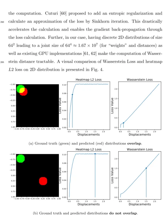
the computation. Cuturi [60] proposed to add an entropic regularization and calculate an approximation of the loss by Sinkhorn iteration. This drastically
260
accelerates the calculation and enables the gradient back-propagation through the loss calculation. Further, in our case, having discrete 2D distributions of size 642 leading to a joint size of 644 ≈ 1.67 × 10⁷ (for “weights” and distances) as
well as existing GPU implementations [61, 62] make the computation of Wasser-stein distance tractable. A visual comparison of WasserWasser-stein Loss and heatmap
265
L2 loss on 2D distribution is presented in Fig. 4.
1.00 0.75 0.50 0.25 0.00 0.25 0.50 0.75 1.00 1.00 0.75 0.50 0.25 0.00 0.25 0.50 0.75 1.00 0.0 0.5 1.0 1.5 2.0
Displacements
0.00 0.02 0.04 0.06 0.08 0.10Loss Value
Heatmap L2 Loss
0.0 0.5 1.0 1.5 2.0Displacements
0.0 0.5 1.0 1.5 2.0Loss Value
Wasserstein Loss
(a) Ground truth (green) and predicted (red) distributions overlap.
1.00 0.75 0.50 0.25 0.00 0.25 0.50 0.75 1.00 1.00 0.75 0.50 0.25 0.00 0.25 0.50 0.75 1.00 0.0 0.5 1.0 1.5 2.0
Displacements
0.00 0.02 0.04 0.06 0.08 0.10Loss Value
Heatmap L2 Loss
0.0 0.5 1.0 1.5 2.0Displacements
0.0 0.5 1.0 1.5 2.0Loss Value
Wasserstein Loss
(b) Ground truth and predicted distributions do not overlap.
Figure 4: Comparison of heatmap L2 loss and Wasserstein loss on 2D distributions. We observe that the value of L2 loss saturates when the two distributions do not overlap. However, the value of Wasserstein Loss continues to increase. The Wasserstein loss is able to better integrate the global geometry on the overall heatmap. (Figure taken from [63] with slight modifications.)
(a) σ = 1. (b) σ = 1.5. (c) σ = 3.
Figure 5: Illustration of ground truth target heatmaps defined by Gaussian functions with different σ.
Using Wasserstein loss for HRM has two advantages: (1) It makes the regres-sion sensitive to the global geometry, thus effectively penalizing predicted acti-vations that appear far away from the ground truth position. (2) When training with the L2 loss, the heatmap is not strictly considered as a distribution as no
270
normalisation applied over the map. When training with the Wasserstein loss, the heatmaps are first passed through a softmax function. That means the sum of all pixel values of an output heatmap is normalised to 1, which is statistically more meaningful as each normalised value represents the probability of a land-mark being at the given position. Moreover, when passed through a softmax
275
function, the pixel values on a heatmap are projected to the e-polynomial space. This highlights the largest pixel value and suppresses other pixels whose values are inferior.
5.2. Smoother target heatmaps
Smoother target heatmaps: To improve convergence and robustness, the
280
values of the ground truth heatmaps of HRMs for facial landmark detection are generally defined by 2D Gaussian functions, where the parameter σ is commonly set to 1 or 1.5 (see Fig. 5).
Intuitively, enlarging σ will implicitly force the HRM to consider a larger local neighborhood in the visual support throughout the different CNN layers.
Therefore, when confronting partial interferences (e.g. occlusion, bad lighting conditions), the model should consider a larger context and thus be more robust to these types of noise. Nonetheless, the Gaussian distribution should not be too spread out to ensure some precision and to avoid touching the map boundaries. We empirically found that σ = 3 is an appropriate setting for facial landmark
290
detection. In our experiments, we systematically demonstrate the effectiveness of using σ = 3 compared to σ = 1 or σ = 1.5 for robust landmark detection under challenging conditions.
5.3. Landmark sampling
Landmark sampling: In the early work of HRM [5, 3], the position of a predicted landmark p is sampled directly at the position of the maximum value of the given heatmap H:
(px, py) = arg max p
(H). (5)
However, this inevitably leads to considerable quantization error because the
295
size of the heatmap is generally smaller than the original image (usually around 4 times). An improvement is to use interpolation and resample the numerical coordinates using 4 neighbouring pixel (bilinear interpolation). We denote this method as “GET MAX”.
Liu et al. discussed in [7] that using a target Gaussian distribution with
300
bigger σ decreases the overall NME. Indeed, using bigger σ flattens the output distribution and therefore obfuscates the position of the peak value. As a result, the predictions are locally less precise.
To compensate this local imprecision when using bigger σ, we propose an-other approach to sample numerical coordinates from the heatmap. Inspired by [57], we propose to use the spatial barycenter of the heatmap:
(px, py) =
Z
q∈Ω
q · H(q) , (6)
where Ω denotes the set of pixel positions on the heatmap. We denote this method as “GET BC” (BaryCenter).
GET BC enables sub-pixel prediction, which effectively improves the local precision of the model trained with Wasserstein loss and big σ. On the other hand, GET BC considers the entire heatmap and thus involves a global context for a more robust final detection.
6. Experiments
310
In this section, we compare our method with other state-of-the-art meth-ods and realize ablation studies using both traditional and proposed evaluation metrics. We also apply our method on various HRMs to demonstrate that our method can be directly used for any structures without further adjustments.
To provide a general idea on the NME and the threshold of FR in this section,
315
we demonstrate the error normalised by inter-ocluar distance at different scales in Fig. 7. The ground truth position is the inner corner of the right eye. The errors within 5% are relatively small ones. From 10%, the errors might be larger than the distance between adjacent landmarks. The errors larger than 20% completely violate the reasonable face shape and needs to be avoided in
320
most applications.
6.1. Effectiveness of barycenter sampling
Effectiveness of barycenter sampling: The GET BC method for esti-mating the predicted landmark coordinates is able to significantly improve the precision of the model trained with Wasserstein loss and larger σ (see Tab. 2,
325
NME is improved from 4.00% to 3.46%).
In contrast, GET BC is not compatible with the output trained with heatmap L2 loss (FRL
0.2is largely increased from 0.58% to 16.83% using GET BC). Please
note that, in Tab. 2, we only compare the sampling methods. Comparision of using different σ and loss functions will be done later in this paper.
330
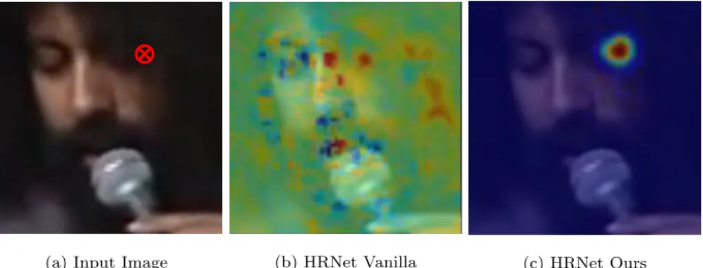
Training with L2 is less robust and generally leads to spurious activations far away from the ground truth position, which prevents GET BC from estimating good positions. Figure 6 shows an example comparing the output heatmaps
σ Loss Method NME(%) FRL 0.05(%)
1 Heatmap L2 GET MAX 3.34 18.33 GET BC 20.15 93.70 3 Wasserstein GET MAX 4.00 24.69
GET BC 3.46 19.42
Table 2: Performance of HRNet on the 300W validation set when using different coordinate sampling methods. GET BC improves the local precision (see FRL
0.05) of the model trained
with Wasserstein loss (W Loss) and large σ. However, it harms the performance of the model trained with Heatmap L2 loss (HM L2).
(a) Input Image (b) HRNet Vanilla (c) HRNet Ours
(a) Input Image (b) HRNet Vanilla (c) HRNet Ours
(a) Input Image (b) HRNet Vanilla (c) HRNet Ours
(a) Input Image (b) HRNet Vanilla (c) HRNet OursFigure 6: Output heatmap comparisons under occlusion. We show the heatmaps of the landmark marked in red.
from a vanilla HRNet (trained with L2 loss, σ = 1) and our HRNet (trained with Wasserstein loss, σ = 3) on a occluded landmark (outer right eye-corner).
335
We observe that our strategy effectively removes the spurious activation on the unrelated regions, so that the prediction will be more robust and GET BC can be effective. Consider that GET BC significantly improves the precision of the landmarks prediction, especially when using large σ is used. Therefore, in the following experiments, we will by default use GET MAX for models trained
340
Red: 5%
Orange: 8%
Green: 10%
Purple: 20%
Figure 7: Demonstration of the nor-malised error from 5% to 20%.
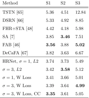
Method S1 S2 S3 TSTN [65] 5.36 4.51 12.84 DSRN [66] 5.33 4.92 8.85 FHR+STA [48] 4.42 4.18 5.98 SA [7] 3.85 3.46 7.51 FAB [46] 3.56 3.88 5.02 DeCaFA [67] 3.82 3.63 6.67 HRNet, σ = 1, L2 3.74 3.73 5.49 σ = 3, L2 3.42 3.58 5.12 σ = 1, W Loss 3.41 3.66 5.01 σ = 3, W Loss 3.39 3.64 4.99 σ = 3, W Loss, CC 3.35 3.61 5.05
Table 3: NME (%) on 300VW. W Loss - Wasser-stein Loss. CC - CoordConv.
6.2. Comparison with the state-of-the-art
Comparison with the state-of-the-art: We performed an ablation study using a “vanilla” HRNet (trained with heatmap L2 loss and σ = 1) as our base-line. We also tested a recent method called CoordConv (CC) [64] to integrate
345
geometric information to the CNN. To this end, we replaced all the convolu-tional layers by CoordConv layers. We benchmark our method with standard evaluation metrics NME on 300VW in Tab. 3, WFLW in Tab. 4, AFLW in Tab. 5 and 300W in Tab. 6 .
On 300VW (Tab. 3), our method shows promising performance, especially
350
under challenging conditions on Scenario 3. On S3, by using Wasserstein loss, the NME drops by 0.48 point. By using a bigger σ, the NME drops by 0.37 point. By using both, the NME can be further improved for a small margin. Using the Wasserstein loss combined with a larger σ, our method outperforms the vanilla HRNet by a significant margin of 0.39%, 0.15% and 0.5% points on
355
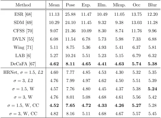
Method Mean Pose Exp. Illm. Mkup. Occ Blur ESR [68] 11.13 25.88 11.47 10.49 11.05 13.75 12.20 SDM [69] 10.29 24.10 11.45 9.32 9.38 13.03 11.28 CFSS [70] 9.07 21.36 10.09 8.30 8.74 11.76 9.96 DVLN [55] 6.08 11.54 6.78 5.73 5.98 7.33 6.88 Wing [71] 5.11 8.75 5.36 4.93 5.41 6.37 5.81 LAB [6] 5.27 10.24 5.51 5.23 5.15 6.79 6.32 DeCaFA [67] 4.62 8.11 4.65 4.41 4.63 5.74 5.38 HRNet, σ = 1.5, L2 4.60 7.77 4.85 4.53 4.30 5.32 5.35 σ = 3, L2 4.76 7.99 4.97 4.62 4.50 5.51 5.39 σ = 1.5, W 4.57 7.76 4.80 4.45 4.37 5.38 5.24 σ = 3, W 4.76 8.01 5.08 4.68 4.61 5.56 5.42 σ = 1.5, W, CC 4.52 7.65 4.72 4.33 4.26 5.27 5.28 σ = 3, W, CC 4.82 8.16 5.11 4.68 4.67 5.57 5.45
Table 4: NME (%) on WFLW. W - Wasserstein Loss. CC - CoordConv.
On WFLW (Tab. 4), our method achieves good performances by using a strong baseline. Nonetheless, using Wasserstein loss (4.57%) only achieves marginal improvement compared to using L2 loss (4.60%). We think that it is because the predictions are already “regularized” by the dense annotation of
360
WFLW. We will analyze this issue in detail in Sect. 7.
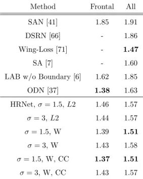
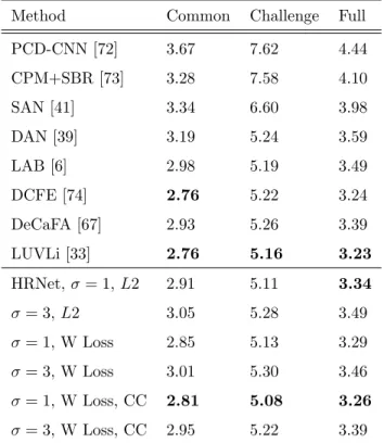
On AFLW (Tab. 5) and 300W (Tab. 6) datasets, our model shows compa-rable performance to the state-of-the-art methods using traditional evaluation metrics. Here, using the Wasserstein loss only achieves a marginal improve-ment. And using a larger σ even slightly decreases the NME performance. As
365
discussed in Sect. 2, the performance of vanilla HRNet has already reached a high level on these datasets. Thus, there are only very few challenging valida-tion images for HRNet. The NME is dominated by a large amount of small errors, which is the disadvantage of using a larger σ, and it can thus no longer reflect the robustness of the models. In the following parts, the robustness of
Method Frontal All SAN [41] 1.85 1.91 DSRN [66] - 1.86 Wing-Loss [71] - 1.47
SA [7] - 1.60
LAB w/o Boundary [6] 1.62 1.85 ODN [37] 1.38 1.63 HRNet, σ = 1.5, L2 1.46 1.57 σ = 3, L2 1.44 1.57 σ = 1.5, W 1.39 1.51 σ = 3, W 1.43 1.58 σ = 1.5, W, CC 1.37 1.51 σ = 3, W, CC 1.43 1.57
Table 5: NME(%) performance comparision on AFLW. W - Wasserstein Loss. CC - Coord-Conv.
these models were validated by using cross-dataset validation.
6.3. Cross-dataset validation
Cross-dataset validation: We use cross-dataset validation to measure the robustness of our HRNet trained on 300W. We present the landmark-wise CEDs of protocol 300W→WFLW (Fig. 8), protocol 300W→300VW (Tab. 7), protocol
375
COFW→AFLW (Fig. 9) and protocol WFLW→300VW (Fig. 10).
From protocol 300W→WFLW (Fig. 8), we find that using larger σ (L2 Loss, σ = 3) and Wasserstein loss (W Loss, σ = 1) can respectively improve the NME by 0.5 point. Using both (W Loss, σ = 3) further improves the NME to be 1 point inferior than the vanilla HRNet. Notably, the improvement on larger errors
380
(error >= 20%) is more significant the the errors < 20%, which demonstrates the superior robustness against large errors of our HRNet compared to vanilla HRNet. From protocol 300W→300VW (Tab. 7), we obtain similar conclusions. Both bigger σ and Wasserstein Loss improve the robustness. The contribution
Method Common Challenge Full PCD-CNN [72] 3.67 7.62 4.44 CPM+SBR [73] 3.28 7.58 4.10 SAN [41] 3.34 6.60 3.98 DAN [39] 3.19 5.24 3.59 LAB [6] 2.98 5.19 3.49 DCFE [74] 2.76 5.22 3.24 DeCaFA [67] 2.93 5.26 3.39 LUVLi [33] 2.76 5.16 3.23 HRNet, σ = 1, L2 2.91 5.11 3.34 σ = 3, L2 3.05 5.28 3.49 σ = 1, W Loss 2.85 5.13 3.29 σ = 3, W Loss 3.01 5.30 3.46 σ = 1, W Loss, CC 2.81 5.08 3.26 σ = 3, W Loss, CC 2.95 5.22 3.39
Table 6: NME (%) comparison on 300W. W Loss - Wasserstein Loss. CC - CoordConv.
of Wasserstein Loss is more important than the larger σ (see FRL0.1). However,
385
even GET BC is used, a larger σ still slightly decreases the local precision. As a result, on the less challenging datasets such as 300VW-S1 and 300VW-S2, we found that the best performance can be obtained by using a combination of small σ, Wasserstein loss and CoordConv. On more challenging datasets such as WFLW and 300VW-S3, the best performance is obtained by using a
390
combination of the Wasserstein loss and a larger σ.
The landmark-wise CED of the protocol COFW→AFLW is presented in Fig. 9. Our method achieves a bigger improvement on COFW→AFLW-All compared to COFW→AFLW-Frontal. This is because AFLW-All contains non-frontal images, which is more challenging than AFLW-Frontal.
395
On COFW→AFLW-All (Fig. 9 (a)), by using Wasserstein loss, the NME performance can be improved by 0.13% from 3.54% to 3.41%. Using CordConv
0.100 0.125 0.150 0.175 0.200 0.225 0.250 0.275 0.300
NME
75
80
85
90
95
Landmark Proportion (%)
Landmark-wise CED on WFLW Valid
L2 Loss, =1,
NME = 9.84
L2 Loss, =3, NME=9.33
W Loss, =1, NME=9.34
W Loss, =3,
NME = 8.84
W Loss, =1, CordConv, NME=9.01
W Loss, =3, CordConv, NME=8.93
Figure 8: Landmark-wise CED of 300W→WFLW validation.
can further improve the performance by 0.08% to 3.33%. Specifically, the im-provement is significant at the NME from 6% to 25%. However, using big σ will still decrease the local precision. We notice that the models using big σ perform
400
worse than the models using small σ at NME=5%.
The landmark-wise CED of the protocol WFLW→300VW is shown in Fig. 10. We observe that by using Wasserstein Loss and CordConv, the HRNet trained on WFLW can be better generalized on the 300VW dataset. However, the im-provement is less significant compared to the protocol 300W→300VW. We will
405
discuss later on in Sect. 7 that, the model trained on WFLW (with the dense an-notation of 98 landmarks) has been already regularized by the strong landmark correlation among adjacent landmarks.
Method Scenario 1 Scenario 2 Scenario 3 NME FRL 0.1 NME FRL0.1 NME FRL0.1 σ = 1, L2 4.44 5.02 4.37 4.86 6.67 11.65 σ = 3, L2 4.36 4.89 4.38 4.83 6.35 10.97 σ = 1, W 4.16 4.68 4.21 4.67 6.31 10.08 σ = 3, W 4.17 4.84 4.16 4.47 6.01 9.91 σ = 1, W, CC 4.05 4.22 4.11 4.26 6.32 10.61 σ = 3, W, CC 4.21 4.78 4.24 4.61 6.02 9.58
Table 7: NME (%) and FRL
0.1 (%) comparision of 300W→300VW cross-dataset validation
using HRNet. W - Wasserstein Loss. CC - CoordConv.
0.05 0.10 0.15 0.20 0.25 0.30 NME 82.5 85.0 87.5 90.0 92.5 95.0 97.5 100.0 Landmark Proportion (%)
Landmark-wise CED on AFLW-All
L2 Loss, =1.5, NME = 3.54
L2 Loss, =3, NME=3.66 W Loss, =1.5, NME=3.41 W Loss, =3, NME=3.55 W Loss, =1.5, CordConv, NME = 3.33
W Loss, =3, CordConv, NME=3.62
(a) COFW→AFLW-All 0.05 0.10 0.15 0.20 0.25 0.30
NME
96.0 96.5 97.0 97.5 98.0 98.5 99.0 99.5Landmark Proportion (%)
Landmark-wise CED on AFLW-Frontal
L2 Loss, =1.5, NME = 2.12 L2 Loss, =3, NME=2.18 W Loss, =1.5, NME = 2.10 W Loss, =3, NME=2.22 W Loss, =1.5, CordConv, NME=2.14 W Loss, =3, CordConv, NME=2.17
(b) COFW→AFLW-Frontal
Figure 9: Landmark-wise CED of COFW→AFLW cross-validation with HRNet.
6.4. Synthetic occlusions and motion blur
Synthetic occlusions and motion blur: We further evaluated the
robust-410
ness against synthetic perturbations that we described in Sect. 4 (see Tab. 8 and Tab. 9). We find that the model is more robust to occlusion and motion blur by using a larger σ and Wasserstein loss. For example, the FRL
0.2is improved from
2.66% to 1.72% under large occlusions. Under large motion blur perturbations, the FRL0.2 is improved from 36.63% to 31.32%.
0.100 0.125 0.150 0.175 0.200 0.225 0.250 0.275 0.300
NME
90 92 94 96 98 100Landmark Proportion (%)
Landmark-wise CED on 300VW-S3
L2 Loss, =1.5, NME = 6.14 L2 Loss, =3, NME=6.14 W Loss, =1.5, NME=6.07 W Loss, =3, NME=6.05W Loss, =1.5, CordConv, NME = 6.01 W Loss, =3, CordConv, NME=6.05
(a) WFLW→300VW-S3 0.100 0.125 0.150 0.175 0.200 0.225 0.250 0.275 0.300
NME
95 96 97 98 99 100Landmark Proportion (%)
Landmark-wise CED on 300VW-S2
L2 Loss, =1.5, NME = 4.25 L2 Loss, =3, NME=4.32 W Loss, =1.5, NME=4.28 W Loss, =3, NME=4.25W Loss, =1.5, CordConv, NME = 4.10 W Loss, =3, CordConv, NME=4.24
(b) WFLW→300VW-S2 0.100 0.125 0.150 0.175 0.200 0.225 0.250 0.275 0.300
NME
94 95 96 97 98 99 100Landmark Proportion (%)
Landmark-wise CED on 300VW-S1
L2 Loss, =1.5, NME = 4.45 L2 Loss, =3, NME=4.47 W Loss, =1.5, NME=4.41 W Loss, =3, NME=4.34W Loss, =1.5, CordConv, NME = 4.26 W Loss, =3, CordConv, NME=4.34
(c) WFLW→300VW-S1
Figure 10: Cross-dataset validation of HRNet trained on WFLW (WFLW→300VW).
6.5. Comparision with other loss functions
Comparision with other loss functions: Besides Heatmap L2, we note that there exists several other loss functions for HRMs. Jensen–Shannon diver-gence (loss) is a common metric for measuring the distance between two proba-bilistic distributions. Soft ArgMax [57] transforms the heatmap regression into
420
a numeric integral regression problem, which we think might be beneficial for model robustness. From Tab. 10, we find that the HRNet trained with Wasser-stein loss delivers more robust predictions compared to the HRNet trained with other loss functions.
Occlusion (300W)
Protocol σ Loss CC NME FRI0.1 FRL0.1 FRL0.15 FRL0.2
Large 1 L2 × 4.63 4.31 10.11 4.83 2.66 3 W × 4.48 2.95 9.62 3.88 1.72 3 W X 4.60 3.79 9.89 4.26 2.03 Medium 1 L2 × 3.57 0.97 5.58 1.94 0.83 3 W × 3.62 0.46 5.46 1.74 0.63 3 W X 3.60 0.58 5.11 1.65 0.61
Table 8: Results of the HRNet with synthetic occlusion (validated on 300W dataset).
Blur (300VW-S3) Protocol σ Loss CC NME FRI
0.1 FRL0.1 FRL0.15 FRL0.2 Large 1 L2 × 27.42 66.3 56.57 44.28 36.63 3 W × 19.15 64.51 54.70 41.03 31.32 3 W X 19.32 63.65 55.71 41.85 31.68 Medium 1 L2 × 11.07 31.67 28.34 15.22 9.32 3 W × 9.5 27.54 27.34 14.35 7.80 3 W X 9.07 25.14 26.37 12.76 6.27
Table 9: Results of the HRNet with synthetic motion blur (validated on 300VW-S3).
6.6. Different models
425
Different models: To demonstrate that our method can be used on a variety of HRMs regardless of the model structure, we test our method on three popular HRMs: HourGlass [5], CPN [75] and SimpleBaselines [76]. In Fig. 11 we can see that all of the three models benefit from our method. This indicates that our approach is quite general and can be applied to most existing HRMs.
430
6.7. Visual comparison
Visual comparison: We visually compare the predictions from vanilla HRNet and our HRNet on a challenging video clip in Fig. 12. Our HRNet gives
Loss Sampling FRI 0.08 FRI0.1 FRL0.08 FRL0.1 FRL0.15 FRL0.2 300W→WFLW JS† GET MAX 40.48 26.24 37.60 26.89 13.72 8.37 JS† GET BC 40.44 26.12 37.49 27.17 14.37 9.04 S. AM† GET BC 42.60 26.40 40.37 29.23 14.86 8.51 W† GET BC 39.24 25.12 37.27 26.61 13.42 8.03 W∗ GET BC 39.96 23.64 37.42 26.39 12.81 7.32 300W→300VW-S3 JS† GET MAX 11.07 5.14 19.27 11.97 4.45 2.06 JS† GET BC 10.87 5.34 18.93 11.92 4.66 2.28 S. AM† GET BC 11.08 5.61 19.00 11.59 4.45 2.09 W† GET BC 9.72 3.73 17.96 11.08 4.15 1.79 W∗ GET BC 7.52 2.96 16.03 9.58 3.39 1.46
Table 10: Cross-dataset validation (300W→WFLW & 300W→300VW) of the HRNet using different loss functions. †: Trained with Gaussian Distribution σ = 1 without CoordConv. ∗: Trained with σ = 3 with CoordConv. JS: Jensen–Shannon divergence (loss). S. AM: Soft ArgMax Loss. W: Wasserstein Loss.
a more robust detection when confronted to extreme poses and motion blur. By using the Wasserstein loss, a larger σ and GET BC, the predicted landmarks
435
are more regularized by the global geometry compared to the prediction from the vanilla HRNet.
7. Discussions
7.1. Dense annotation
Does dense annotation naturally ensure the robustness? We find
440
that our method shows less significant improvement on the model trained on WFLW. Intuitively, we presume that by training with a dense annotation (98 landmarks), the model predictions are somewhat regularized by the correlation between neighbouring landmarks. In Tab. 11, we compare the models trained
0.100 0.125 0.150 0.175 0.200 0.225 0.250 0.275 0.300
NME
70 75 80 85 90 95Landmark Proportion (%)
Landmark-wise CED on WFLW
HG: L2 Loss, =1, NME=9.33 HG: W Loss, =3, NME = 8.56 CPN: L2 Loss, =1, NME=11.30 CPN: W Loss, =3, NME = 10.04 SB: L2 Loss, =1, NME=11.26 SB: W Loss, =3, NME = 9.97 (a) 300W→WFLW 0.100 0.125 0.150 0.175 0.200 0.225 0.250 0.275 0.300NME
88 90 92 94 96 98 100Landmark Proportion (%)
Landmark-wise CED on 300VW-S3
HG: L2 Loss, =1, NME=6.09 HG: W Loss, =3, NME = 5.64 CPN: L2 Loss, =1, NME=7.30 CPN: W Loss, =3, NME = 7.00 SB: L2 Loss, =1, NME=7.27 SB: W Loss, =3, NME = 6.58 (b) 300W→300VW-S3 Figure 11: Cross-dataset validation of HG [5], CPN [75] and SimpleBaselines(SB) [76].HRNet
Vanilla
HRNet
Ours
Figure 12: Visual comparison of vanilla HRNet (L2 Loss and σ = 1) and our HRNet (Wasser-stein loss and σ = 3).
with different number of landmarks. The 68 landmark format is a subset of
445
the original 98 landmark format, which is similar to the 300W annotation. The 17 landmark format is a subset of the 68 landmark format, which is similar to the AFLW annotation (except the eye centers). To ensure the fair comparison, though trained with different number of landmarks, all the models listed are tested on the common 17 landmarks. We found that the prediction is naturally
450
more robust by training with denser annotation formats. Therefore, compared to the model trained with more sparse annotation, our method achieves less important improvement on the model trained with dense annotation.
N. Landmks σ Loss FRL 0.15 FRL0.2 17 1 L2 2.79 1.60 3 W 2.68 1.29 68 1 L2 0.65 0.37 3 W 0.62 0.33 98 1 L2 0.44 0.25 3 W 0.43 0.22
Table 11: Comparison of HRNets trained with different number of landmarks on WFLW. W: Wasserstein Loss.
7.2. Recommended settings
We recommend to use the Wasserstein loss and GET BC to improve the
455
robustness of the model in all cases. Using a larger σ will significantly improve the robustness under challenging conditions. Nonetheless, it deteriorates the local precision at the same time. In fact, the value of σ is a trade-off between robustness and precision. Therefore, we recommend to use a larger σ only when confronting crucial circumstances. When facing less challenging conditions, we
460
recommend to use a combination of Wasserstein loss and small σ. Complement-ing CoordConv with Wasserstein loss and small σ will further improve the NME performance. However, it adds slight computational complexity to the HRMs. Specifically, when using small σ, the models with CoordConv are less robust against large occlusions compared to those without CoordConv.
465
7.3. Strengths and Weaknesses:
Strengths: Our method is simple and efficient. It significantly improves the robustness without introducing any structural modification or complexity during the inference stage.
Weaknesses: During training, the calculation of Wasserstein loss is
rel-470
atively time-consuming, even with GPU. We also tested our method for the task of human pose estimation, we do not observe improvement on the MPII
dataset [77]. It is probably due to the fact that human joints have more artic-ulations and left/right confusions than facial landmarks, thus involving limited geometric information and global context.
475
Future work can be focused on how to generalize this approach on more complicated tasks such as human pose estimation.
8. Conclusions
In this paper, we studied the problem of robust facial landmark detection regarding several aspects such as the use of datasets, evaluation metrics and
480
methodology. Due to the performance saturation, we found that the widely used FR and NME measures can no longer effectively reflect the robustness of a model on several popular benchmarks. Therefore, we proposed several modifications to the current evaluation metrics and a novel method to make HRMs more robust. Our approach is based on the Wasserstein loss and involves training
485
with smoother target heatmaps as well as a more precise coordinate sampling method using the barycenter of the output heatmaps.
Acknowledgement: This research is funded by the Auvergne Regional Council and the European funds of regional development (FEDER). The com-putation resource is supported by M´esocentre Clermont Auvergne. We would
490
like to thank Nvidia for a GPU donation.
References
[1] S. Duffner, C. Garcia, A connexionist approach for robust and precise facial feature detection in complex scenes, in: International Symposium on Image and Signal Processing and Analysis (ISPA), 2005.
495
[2] C. Villani, Optimal transport: old and new, Vol. 338, Springer Science & Business Media, 2008.
[3] A. Bulat, G. Tzimiropoulos, How far are we from solving the 2d & 3d face alignment problem?(and a dataset of 230,000 3d facial landmarks), in: The IEEE International Conference on Computer Vision (ICCV), 2017.
[4] A. Bulat, G. Tzimiropoulos, Binarized convolutional landmark localizers for human pose estimation and face alignment with limited resources, in: The IEEE International Conference on Computer Vision (ICCV), 2017. [5] A. Newell, K. Yang, J. Deng, Stacked hourglass networks for human pose
estimation, in: European Conference on Computer Vision (ECCV), 2016.
505
[6] W. Wu, C. Qian, S. Yang, Q. Wang, Y. Cai, Q. Zhou, Look at boundary: A boundary-aware face alignment algorithm, in: The IEEE Conference on Computer Vision and Pattern Recognition (CVPR), 2018.
[7] Z. Liu, X. Zhu, G. Hu, H. Guo, M. Tang, Z. Lei, N. M. Robertson, J. Wang, Semantic alignment: Finding semantically consistent ground-truth for
fa-510
cial landmark detection, in: The IEEE Conference on Computer Vision and Pattern Recognition (CVPR), 2019.
[8] A. Dapogny, K. Bailly, M. Cord, Decafa: Deep convolutional cascade for face alignment in the wild, in: The IEEE International Conference on Com-puter Vision (ICCV), 2019.
515
[9] K. Sun, Y. Zhao, B. Jiang, T. Cheng, B. Xiao, D. Liu, Y. Mu, X. Wang, W. Liu, J. Wang, High-resolution representations for labeling pixels and regions, arXiv preprint arXiv:1904.04514.
[10] J. Deng, G. Trigeorgis, Y. Zhou, S. Zafeiriou, Joint multi-view face align-ment in the wild, IEEE Transactions on Image Processing 28 (7) (2019)
520
3636–3648.
[11] Z. Tang, X. Peng, S. Geng, L. Wu, S. Zhang, D. Metaxas, Quantized densely connected u-nets for efficient landmark localization, in: European Conference on Computer Vision (ECCV), 2018.
[12] X. P. Burgos-Artizzu, P. Perona, P. Doll´ar, Robust face landmark
estima-525
tion under occlusion, in: The IEEE International Conference on Computer Vision (ICCV), 2013.
[13] A. Asthana, S. Zafeiriou, S. Cheng, M. Pantic, Robust discriminative re-sponse map fitting with constrained local models, in: The IEEE Conference on Computer Vision and Pattern Recognition (CVPR), 2013.
530
[14] B. M. Smith, J. Brandt, Z. Lin, L. Zhang, Nonparametric context mod-eling of local appearance for pose-and expression-robust facial landmark localization, in: The IEEE Conference on Computer Vision and Pattern Recognition (CVPR), 2014.
[15] X. Zhao, S. Shan, X. Chai, X. Chen, Cascaded shape space pruning for
535
robust facial landmark detection, in: The IEEE International Conference on Computer Vision (ICCV), 2013.
[16] X. Yu, Z. Lin, J. Brandt, D. N. Metaxas, Consensus of regression for occlusion-robust facial feature localization, in: European Conference on Computer Vision (ECCV), 2014.
540
[17] Y. Wu, C. Gou, Q. Ji, Simultaneous facial landmark detection, pose and deformation estimation under facial occlusion, in: The IEEE Conference on Computer Vision and Pattern Recognition (CVPR), 2017.
[18] F. Zhou, J. Brandt, Z. Lin, Exemplar-based graph matching for robust facial landmark localization, in: The IEEE Conference on Computer Vision
545
and Pattern Recognition (CVPR), 2013.
[19] Z.-H. Feng, J. Kittler, M. Awais, P. Huber, X.-J. Wu, Face detection, bounding box aggregation and pose estimation for robust facial landmark localisation in the wild, in: The IEEE Conference on Computer Vision and Pattern Recognition Workshop (CVPRW), 2017.
550
[20] H. Yang, X. He, X. Jia, I. Patras, Robust face alignment under occlu-sion via regional predictive power estimation, IEEE Transactions on Image Processing 24 (8) (2015) 2393–2403.
[21] Y. Wu, Q. Ji, Robust facial landmark detection under significant head poses and occlusion, in: The IEEE International Conference on Computer Vision
555
(ICCV), 2015.
[22] T. Baltrusaitis, P. Robinson, L.-P. Morency, Constrained local neural fields for robust facial landmark detection in the wild, in: The IEEE International Conference on Computer Vision Workshop (ICCVW), 2013.
[23] Active appearance models, IEEE Transactions on Pattern Analysis and
560
Machine Intelligence (TPAMI) 23 (6) (2001) 681–685.
[24] D. Cristinacce, T. F. Cootes, Feature detection and tracking with con-strained local models., in: The British Machine Vision Conference (BMVC), 2006.
[25] P. N. Belhumeur, D. W. Jacobs, D. J. Kriegman, N. Kumar, Localizing
565
parts of faces using a consensus of exemplars, IEEE Transactions on Pattern Analysis and Machine Intelligence (TPAMI) 35 (12) (2013) 2930–2940. [26] P. Doll´ar, P. Welinder, P. Perona, Cascaded pose regression, in: The IEEE
Conference on Computer Vision and Pattern Recognition (CVPR), 2010. [27] H. J. Lee, S. T. Kim, H. Lee, Y. M. Ro, Lightweight and effective
fa-570
cial landmark detection using adversarial learning with face geometric map generative network, IEEE Transactions on Circuits and Systems for Video Technology 30 (3) (2019) 771–780.
[28] J. M. Saragih, S. Lucey, J. F. Cohn, Deformable model fitting by regularized landmark mean-shift, International Journal of Computer Vision (IJCV)
575
91 (2) (2011) 200–215.
[29] D. Merget, M. Rock, G. Rigoll, Robust facial landmark detection via a fully-convolutional local-global context network, in: The IEEE Conference on Computer Vision and Pattern Recognition (CVPR), 2018.
[30] L. Chen, H. Su, Q. Ji, Face alignment with kernel density deep neural
net-580
work, in: The IEEE International Conference on Computer Vision (ICCV), 2019.
[31] X. Wang, L. Bo, L. Fuxin, Adaptive wing loss for robust face alignment via heatmap regression, in: The IEEE International Conference on Computer Vision (ICCV), 2019.
585
[32] X. Zou, S. Zhong, L. Yan, X. Zhao, J. Zhou, Y. Wu, Learning robust facial landmark detection via hierarchical structured ensemble, in: The IEEE International Conference on Computer Vision (ICCV), 2019.
[33] A. Kumar, T. K. Marks, W. Mou, Y. Wang, M. Jones, A. Cherian, T. Koike-Akino, X. Liu, C. Feng, Luvli face alignment: Estimating
land-590
marks’ location, uncertainty, and visibility likelihood, in: The IEEE Con-ference on Computer Vision and Pattern Recognition (CVPR), 2020. [34] J. Wan, Z. Lai, J. Liu, J. Zhou, C. Gao, Robust face alignment by
multi-order high-precision hourglass network, IEEE Transactions on Image Pro-cessing 30 (2020) 121–133.
595
[35] J. Wan, Z. Lai, J. Li, J. Zhou, C. Gao, Robust facial landmark detection by multiorder multiconstraint deep networks, IEEE Transactions on Neural Networks and Learning Systems (2021) 1–14.
[36] H. Park, D. Kim, Acn: Occlusion-tolerant face alignment by attentional combination of heterogeneous regression networks, Pattern Recognition
600
(2020) 107761.
[37] M. Zhu, D. Shi, M. Zheng, M. Sadiq, Robust facial landmark detection via occlusion-adaptive deep networks, in: The IEEE Conference on Computer Vision and Pattern Recognition (CVPR), 2019.
[38] S. Xiao, J. Feng, J. Xing, H. Lai, S. Yan, A. Kassim, Robust facial
land-605
mark detection via recurrent attentive-refinement networks, in: European Conference on Computer Vision (ECCV), 2016.
[39] M. Kowalski, J. Naruniec, T. Trzcinski, Deep alignment network: A convo-lutional neural network for robust face alignment, in: The IEEE Conference on Computer Vision and Pattern Recognition Workshop (CVPRW), 2017.
610
[40] J. Yang, Q. Liu, K. Zhang, Stacked hourglass network for robust facial landmark localisation, in: The IEEE Conference on Computer Vision and Pattern Recognition Workshop (CVPRW), 2017.
[41] X. Dong, Y. Yan, W. Ouyang, Y. Yang, Style aggregated network for facial landmark detection, in: The IEEE Conference on Computer Vision and
615
Pattern Recognition (CVPR), 2018.
[42] J. Zhang, H. Hu, S. Feng, Robust facial landmark detection via heatmap-offset regression, IEEE Transactions on Image Processing 29 (2020) 5050– 5064.
[43] L. Chen, H. Su, Q. Ji, Deep structured prediction for facial landmark
detec-620
tion, in: The Conference and Workshop on Neural Information Processing Systems (NeurIPS), 2019.
[44] X. Zou, P. Xiao, J. Wang, L. Yan, S. Zhong, Y. Wu, Towards unconstrained facial landmark detection robust to diverse cropping manners, IEEE Trans-actions on Circuits and Systems for Video Technology (2020) 1–1.
625
[45] Z. Tong, J. Zhou, Face alignment using two-stage cascaded pose regression and mirror error correction, Pattern Recognition (2021) 107866.
[46] K. Sun, W. Wu, T. Liu, S. Yang, Q. Wang, Q. Zhou, Z. Ye, C. Qian, Fab: A robust facial landmark detection framework for motion-blurred videos, in: The IEEE International Conference on Computer Vision (ICCV), 2019.
630
[47] H. Zhu, H. Liu, C. Zhu, Z. Deng, X. Sun, Learning spatial-temporal de-formable networks for unconstrained face alignment and tracking in videos, Pattern Recognition 107 (2020) 107354.
[48] Y. Tai, Y. Liang, X. Liu, L. Duan, J. Li, C. Wang, F. Huang, Y. Chen, To-wards highly accurate and stable face alignment for high-resolution videos,
635
in: AAAI Conference on Artificial Intelligence, 2019.
[49] C. Sagonas, G. Tzimiropoulos, S. Zafeiriou, M. Pantic, 300 faces in-the-wild challenge: The first facial landmark localization challenge, in: The IEEE Conference on Computer Vision and Pattern Recognition Workshop (CVPRW), 2013.
640
[50] P. M. R. Martin Koestinger, Paul Wohlhart, H. Bischof, Annotated Facial Landmarks in the Wild: A Large-scale, Real-world Database for Facial Landmark Localization, in: Proc. First IEEE International Workshop on Benchmarking Facial Image Analysis Technologies, 2011.
[51] J. Shen, S. Zafeiriou, G. G. Chrysos, J. Kossaifi, G. Tzimiropoulos, M.
Pan-645
tic, The first facial landmark tracking in-the-wild challenge: Benchmark and results, in: The IEEE International Conference on Computer Vision Workshop (ICCVW), 2015.
[52] B. M. Smith, L. Zhang, Collaborative facial landmark localization for trans-ferring annotations across datasets, in: European Conference on Computer
650
Vision (ECCV), 2014.
[53] S. Zhu, C. Li, C. C. Loy, X. Tang, Transferring landmark annotations for cross-dataset face alignment, arXiv preprint arXiv:1409.0602.
[54] J. Zhang, M. Kan, S. Shan, X. Chen, Leveraging datasets with varying annotations for face alignment via deep regression network, in: The IEEE
655
International Conference on Computer Vision (ICCV), 2015.
[55] W. Wu, S. Yang, Leveraging intra and inter-dataset variations for robust face alignment, in: The IEEE Conference on Computer Vision and Pattern Recognition Workshop (CVPRW), 2017.
[56] X. Liu, Z. Hu, H. Ling, Y. M. Cheung, Mtfh: A matrix tri-factorization
660
Transac-tions on Pattern Analysis and Machine Intelligence (TPAMI) 43 (3) (2021) 964–981.
[57] X. Sun, B. Xiao, F. Wei, S. Liang, Y. Wei, Integral human pose regression, in: European Conference on Computer Vision (ECCV), 2018.
665
[58] Differential earth mover’s distance with its applications to visual tracking, IEEE Transactions on Pattern Analysis and Machine Intelligence (TPAMI) 32 (2) (2010) 274–287.
[59] G. Yao, A. Dani, Visual tracking using sparse coding and earth mover’s distance, Frontiers in Robotics and AI 5.
670
[60] M. Cuturi, Sinkhorn distances: Lightspeed computation of optimal trans-port, in: The Conference and Workshop on Neural Information Processing Systems (NeurIPS), 2013.
[61] T. Viehmann, Implementation of batched sinkhorn iterations for entropy-regularized wasserstein loss, arXiv preprint arXiv:1907.01729.
675
[62] D. Daza, Approximating wasserstein distances with pytorch, https:// dfdazac.github.io/sinkhorn.html (2019).
[63] C. Tralie, 2d histogram wasserstein distance via pot library, https://gist. github.com/ctralie/66352ae6ab06c009f02c705385a446f3 (2018). [64] R. Liu, J. Lehman, P. Molino, F. P. Such, E. Frank, A. Sergeev, J. Yosinski,
680
An intriguing failing of convolutional neural networks and the coordconv solution, in: The Conference and Workshop on Neural Information Pro-cessing Systems (NeurIPS), 2018.
[65] Two-stream transformer networks for video-based face alignment, IEEE Transactions on Pattern Analysis and Machine Intelligence (TPAMI)
685
[66] X. Miao, X. Zhen, X. Liu, C. Deng, V. Athitsos, H. Huang, Direct shape re-gression networks for end-to-end face alignment, in: The IEEE Conference on Computer Vision and Pattern Recognition (CVPR), 2018.
[67] A. Dapogny, K. Bailly, M. Cord, Decafa: Deep convolutional cascade for
690
face alignment in the wild, in: The IEEE International Conference on Com-puter Vision (ICCV), 2019.
[68] X. Cao, Y. Wei, F. Wen, J. Sun, Face alignment by explicit shape regression, International Journal of Computer Vision (IJCV) 107 (2) (2014) 177–190. [69] X. Xiong, F. De la Torre, Supervised descent method and its applications to
695
face alignment, in: The IEEE Conference on Computer Vision and Pattern Recognition (CVPR), 2013.
[70] S. Zhu, C. Li, C. Change Loy, X. Tang, Face alignment by coarse-to-fine shape searching, in: The IEEE Conference on Computer Vision and Pattern Recognition (CVPR), 2015.
700
[71] Z.-H. Feng, J. Kittler, M. Awais, P. Huber, X.-J. Wu, Wing loss for robust facial landmark localisation with convolutional neural networks, in: The IEEE Conference on Computer Vision and Pattern Recognition (CVPR), 2018.
[72] A. Kumar, R. Chellappa, Disentangling 3d pose in a dendritic cnn for
705
unconstrained 2d face alignment, in: The IEEE Conference on Computer Vision and Pattern Recognition (CVPR), 2018.
[73] X. Dong, S.-I. Yu, X. Weng, S.-E. Wei, Y. Yang, Y. Sheikh, Supervision-by-registration: An unsupervised approach to improve the precision of facial landmark detectors, in: The IEEE Conference on Computer Vision and
710
Pattern Recognition (CVPR), 2018.
[74] R. Valle, J. M. Buenaposada, A. Vald´es, L. Baumela, A deeply-initialized coarse-to-fine ensemble of regression trees for face alignment, in: European Conference on Computer Vision (ECCV), 2018.
[75] Y. Chen, Z. Wang, Y. Peng, Z. Zhang, G. Yu, J. Sun, Cascaded pyramid
715
network for multi-person pose estimation, in: The IEEE Conference on Computer Vision and Pattern Recognition (CVPR), 2018.
[76] B. Xiao, H. Wu, Y. Wei, Simple baselines for human pose estimation and tracking, in: European Conference on Computer Vision (ECCV), 2018. [77] M. Andriluka, L. Pishchulin, P. Gehler, B. Schiele, 2d human pose
es-720
timation: New benchmark and state of the art analysis, in: The IEEE Conference on Computer Vision and Pattern Recognition (CVPR), 2014.