Introduction to the Modern Calculus of Variations pdf - Web Education

(1)

MA4G6 Lecture Notes

Introduction to the

Modern Calculus of Variations

Filip Rindler

(2)

University of Warwick Coventry CV4 7AL United Kingdom

F.Rindler@warwick.ac.uk

http://www.warwick.ac.uk/filiprindler

(3)

Preface

These lecture notes, written for the MA4G6 Calculus of Variations course at the University of Warwick, intend to give a modern introduction to the Calculus of Variations. I have tried to cover different aspects of the field and to explain how they fit into the “big picture”. This is not an encyclopedic work; many important results are omitted and sometimes I only present a special case of a more general theorem. I have, however, tried to strike a balance between a pure introduction and a text that can be used for later revision of forgotten material.

The presentation is based around a few principles:

• The presentation is quite “modern” in that I use several techniques which are perhaps not usually found in an introductory text or that have only recently been developed. • For most results, I try to use “reasonable” assumptions, not necessarily minimal ones. • When presented with a choice of how to prove a result, I have usually preferred the (in my opinion) most conceptually clear approach over more “elementary” ones. For example, I use Young measures in many instances, even though this comes at the expense of a higher initial burden of abstract theory.

• Wherever possible, I first present an abstract result for general functionals defined on Banach spaces to illustrate the general structure of a certain result. Only then do I specialize to the case of integral functionals on Sobolev spaces.

• I do not attempt to trace every result to its original source as many results have evolved over generations of mathematicians. Some pointers to further literature are given in the last section of every chapter.

Most of what I present here is not original, I learned it from my teachers and col-leagues, both through formal lectures and through informal discussions. Published works that influenced this course were the lecture notes on microstructure by S. M¨uller [73], the encyclopedic work on the Calculus of Variations by B. Dacorogna [25], the book on Young measures by P. Pedregal [81], Giusti’s more regularity theory-focused introduction to the Calculus of Variations [44], as well as lecture notes on several related courses by J. Ball, J. Kristensen, A. Mielke. Further texts on the Calculus of Variations are the elementary introductions by B. van Brunt [96] and B. Dacorogna [26], the more classical two-part trea-tise [39, 40] by M. Giaquinta & S. Hildebrandt, as well as the comprehensive treatment of

(4)

the geometric measure theory aspects of the Calculus of Variations by Giaquinta, Modica & Souˇcek [41, 42].

In particular, I would like to thank Alexander Mielke and Jan Kristensen, who are re-sponsible for my choice of research area. Through their generosity and enthusiasm in shar-ing their knowledge they have provided me with the foundation for my study and research. Furthermore, I am grateful to Richard Gratwick and the participants of the MA4G6 course for many helpful comments, corrections, and remarks.

These lecture notes are a living document and I would appreciate comments, corrections and remarks – however small. They can be sent back to me via e-mail at

F.Rindler@warwick.ac.uk or anonymously via

http://tinyurl.com/MA4G6-2015 or by scanning the following QR-Code:

Moreover, every page contains its individual QR-code for immediate feedback. I encourage all readers to make use of them.

F. R. January 2015

(5)

Introduction

Physical modeling is a delicate business – trying to balance the validity of the resulting model, that is, its agreement with nature and its predictive capabilities, with the feasibility of its mathematical treatment is often highly non-straightforward. In this quest to formulate a useful picture of an aspect of the world, it turns out on surprisingly many occasions that the formulation of the model becomes clearer, more compact, or more descriptive, if one introduces some form of a variational principle, that is, if one can define a quantity, such as energy or entropy, which obeys a minimization, maximization or saddle-point law.

How “fundamental” such a scalar quantity is perceived depends on the situation: For example, in classical mechanics, one calls forces conservative if they can be expressed as the derivative of an “energy potential” along a curve. It turns out that many, if not most, forces in physics are conservative, which seems to imply that the concept of energy is fun-damental. Furthermore, Einstein’s famous formula E = mc2 expresses the equivalence of mass and energy, positioning energy as the “most” fundamental quantity, with mass becom-ing “condensed” energy. On the other hand, the other ubiquitous scalar physical quantity, the entropy, has a more “artificial” flavor as a measure of missing information in a model, as is now well understood in Statistical Mechanics, where entropy becomes a derived quan-tity. We leave it to the field of Philosophy of Science to understand the nature of variational concepts. In the words of William Thomson, the Lord Kelvin1:

The fact that mathematics does such a good job of describing the Universe is a mystery that we don’t understand. And a debt that we will probably never be able to repay.

Our approach to variational quantities here is a pragmatic one: We see them as providing structure to a problem and to enable different mathematical, so-called variational, methods. For instance, in elasticity theory it is usually unrealistic that a system will tend to a global minimizer by itself, but this does not mean that – as an approximation – such a principle cannot be useful in practice. On a fundamental level, there probably is no minimization as such in physics, only quantum-mechanical interactions (or whatever lies “below” quantum

(8)

mechanics). However, if we wait long enough, the inherent noise in a realistic system will move our system around and it will settle with a high probability in a low-energy state.

In this course, we will focus solely on minimization problems for integral functionals of the form (Ω ⊂ Rd open and bounded)

∫

Ωf (x, u(x),∇u(x)) dx → min, u :Ω → R

m_,

possibly under conditions on the boundary values of u and further side constraints. These problems form the original core of the Calculus of Variations and are as relevant today as they have always been. The systematic understanding of these integral functionals starts in Euler’s and Bernoulli’s times in the late 1600s and the early 1700s, and their study was boosted into the modern age by Hilbert’s 19th, 20th, 23rd problems, formulated in 1900 [47]. The excitement has never stopped since and new and important discoveries are made every year.

We start this course by looking at a parade of examples, which we treat at varying levels of detail. All these problems will be investigated further along the course once we have developed the necessary mathematical tools.

1.1 The brachistochrone problem

In June 1696 Johann Bernoulli published a problem in the journal Acta Eruditorum, which can be seen as the time of birth of the Calculus of Variations (the name, however, is from Leonhard Euler’s 1766 treatise Elementa calculi variationum). Additionally, Bernoulli sent a letter containing the question to Gottfried Wilhelm Leibniz on 9 June 1696, who returned his solution only a few days later on 16 June, and commented that the problem tempted him “like the apple tempted Eve” because of its beauty. Isaac Newton published a solution (after the problem had reached him) without giving his identity, but Bernoulli identified him “ex ungue leonem” (from Latin, “by the lion’s claw”). The problem was formulated as follows2:

Given two points A and B in a vertical [meaning “not horizontal”] plane, one shall find a curve AMB for a movable point M, on which it travels from A to B in the shortest time, only driven by its own weight.

The resulting curve is called the brachistochrone (from Ancient Greek, “shortest time”) curve.

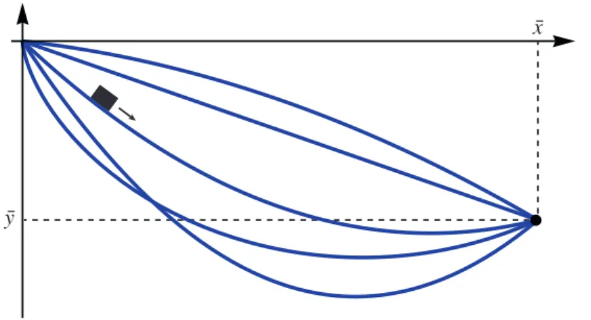
We formulate the problem as follows: We look for the curve y connecting the origin (0, 0) to the point ( ¯x, ¯y), where ¯x > 0, ¯y < 0, such that a point mass m > 0 slides from rest at (0, 0) to ( ¯x, ¯y) quickest among all such curves. See Figure 1.1 for several possible slide paths. We parametrize a point (x, y) on the curve by the time t≥ 0. The point mass has

2_{The German original reads “Wenn in einer verticalen Ebene zwei Punkte A und B gegeben sind, soll}

man dem beweglichen Punkte M eine Bahn AMB anweisen, auf welcher er von A ausgehend verm¨oge seiner eigenen Schwere in k¨urzester Zeit nach B gelangt.”

(9)

1.1. THE BRACHISTOCHRONE PROBLEM 3

Figure 1.1: Several slide curves from the origin to ( ¯x, ¯y).

kinetic and potential energies Ekin= m 2 {( dx dt )2 + ( dy dt )2} =m 2 ( dx dt )2{ 1 + ( dy dx )2} , Epot= mgy,

where g≈ 9.81m/s2is the (constant) gravitational acceleration on Earth. The total energy Ekin+ Epotis zero at the beginning and conserved along the path. Hence, for all y we have

m 2 ( dx dt )2{ 1 + ( dy dx )2} =−mgy.

We can solve this for dt/dx (where t = t(x) is the inverse of the x-parametrization) to get dt dx= √ 1 + (y′)2 −2gy ( dt dx ≥ 0 ) ,

where we wrote y′= dy_dx. Integrating over the whole x-length along the curve from 0 to ¯x, we get for the total time duration T [y] that

T [y] =√1 2g ∫ _x_¯ 0 √ 1 + (y′)2 −y dx.

We may drop the constant in front of the integral, which does not influence the minimization problem, and set ¯x = 1 by reparametrization, to arrive at the problem

     F [y] :=∫ 1 0 √ 1 + (y′)2 −y dx → min, y(0) = 0, y(1) = ¯y < 0.

(10)

Clearly, the integrand is convex in y′, which will be important for the solution theory. We will come back to this problem in Example 2.34.

A related problem concerns Fermat’s Principle expressing that light (in vacuum or in a medium) always takes the fastest path between two points, from which many optical laws, e.g. about reflection and refraction, can be derived.

1.2 Electrostatics

Consider an electric charge densityρ : R3→ R (in units of C/m3) in three-dimensional vacuum. Let E : R3→ R3(in V/m) and B : R3→ R3 (in T = Vs/m2) be the electric and magnetic fields, respectively, which we assume to be constant in time (hence electrostatics). Assuming thatR3 is a linear, homogeneous, isotropic electric material, the Gauss law for electricity reads

∇ · E = divE = ρ ε0 ,

whereε0≈ 8.854 · 10−12C/(Vm). Moreover, we have the Faraday law of induction ∇ × E = curlE =dB

dt = 0.

Thus, since E is curl-free, there exist an electric potentialφ : R3→ R (in V) such that E =−∇φ.

Combining this with the Gauss law, we arrive at the Poisson equation, ∆φ = ∇ · [∇φ] = −_ερ

0

. (1.1)

We can also look at electrostatics in a variational way: We use the norming condition φ(0) = 0. Then, the electric potential energy UE(x; q) of a point charge q > 0 (in C) at point

x∈ R3 in the electric field E is given by the path integral (which does not depend on the path chosen since E is a gradient)

UE(x; q) =− ∫ x 0 qE· ds = − ∫ 1 0 qE(hx) dh = qφ(x).

Thus, the total electric energy of our charge distributionρ is (the factor 1/2 is necessary to count mutual reaction forces correctly)

UE := 1 2 ∫ R3ρφ dx = ε0 2 ∫ R3(∇ · E)φ dx,

which has units of CV = J. Using (∇ · E)φ = ∇ · (Eφ) − E · (∇φ), the divergence theorem, and the natural assumption thatφ vanishes at infinity, we get further

UE =ε0 2 ∫ R3∇ · (Eφ) − E · (∇φ) dx = − ε0 2 ∫ R3E· (∇φ) dx = ε0 2 ∫ R3|∇φ| 2_dx.

(11)

1.3. STATIONARY STATES IN QUANTUM MECHANICS 5

The integral∫_Ω|∇φ|2dx is called Dirichlet integral.

In Example 2.15 we will see that (1.1) is equivalent to the minimization problem UE+ ∫ R3ρφ dx = ∫ R3 ε0 2|∇φ| 2₊_{ρφ dx → min.}

The second term is the energy stored in the electric field caused by its interaction with the charge densityρ.

1.3 Stationary states in quantum mechanics

The non-relativistic evolution of a quantum mechanical system with N degrees of freedom in an electrical field is described completely through its wave function Ψ: RN× R → C that satisfies the Schr¨odinger equation

i¯hd dtΨ(x,t) = [ −¯h 2µ∆ +V(x,t) ] Ψ(x,t), x∈ RN, t∈ R,

where ¯h≈ 1.05 · 10−34Js is the reduced Planck constant, µ > 0 is the reduced mass, and V = V (x,t)∈ R is the potential energy. The (self-adjoint) operator H := −(2µ)−1¯h∆+V is called the Hamiltonian of the system.

The value of the wave function itself at a given point in spacetime has no physical inter-pretation, but according to the Copenhagen Interpretation of quantum mechanics,|Ψ(x)|2 is the probability density of finding a particle at the point x. In order for|Ψ|2to be a proba-bility density, we need to impose the side constraint

∥Ψ∥L2 = 1.

In particular,Ψ(x,t) has to decay as |x| → ∞.

Of particular interest are the so-called stationary states, that is, solutions of the station-ary Schr¨odinger equation

[ −¯h2

2µ ∆ +V(x) ]

Ψ(x) = EΨ(x), x∈ RN,

where E > 0 is an energy level. We then solve this eigenvalue problem (in a weak sense) for Ψ ∈ W1,2_(RN_{;C) with ∥Ψ∥}

L2= 1 (see Appendix A.4 for a collection of facts about Sobolev

spaces like W1,2).

If we are just interested in the lowest-energy state, the so-called ground state, we can find minimizers of the energy functional

E [Ψ] :=∫ RN ¯h2 2µ|∇Ψ(x)| 2₊1 2V (x)|Ψ(x)| 2_dx,

again under the side constraint ∥Ψ∥L2 = 1.

The two parts of the integral above correspond to kinetic and potential energy, respectively. We will continue this investigation in Example 2.39.

(12)

1.4 Hyperelasticity

Elasticity theory is one of the most important theories of continuum mechanics, that is, the study of the mechanics of (idealized) continuous media. We will not go into much detail about elasticity modeling here and refer to the book [20] for a thorough introduction.

Consider a body of mass occupying a domain Ω ⊂ R3, called the reference configu-ration. If we deform the body, any material point x∈ Ω is mapped into a spatial point y(x)∈ R3and we call y(Ω) the deformed configuration. For a suitable continuum mechan-ics theory, we also need to require that y :Ω → y(Ω) is a differentiable bijection and that it is orientation-preserving, i.e. that

det∇y(x) > 0 for all x∈ Ω.

For convenience one also introduces the displacement u(x) := y(x)− x.

One can show (using the implicit function theorem and the mean value theorem) that the orientation-preserving condition and the invertibility are satisfied if

sup

x∈Ω

|∇u(x)| <δ(Ω) (1.2)

for a domain-dependent (small) constantδ(Ω) > 0.

Next, we need a measure of local “stretching”, called a strain tensor, which should serve as the parameter to a local energy density. On physical grounds, rigid body motions, that is, deformations u(x) = Rx + u0with a rotation R∈ R3×3(RT= R−1and det R = 1) and u0∈ R3, should not cause strain. In this sense, strain measures the deviation of the displacement from a rigid body motion. One popular choice is the Green–St. Venant strain tensor3

E :=1 2 (

∇u + ∇uT₊_∇uT_∇u)_. _(1.3)

We first consider fully nonlinear (“finite strain”) elasticity. For our purposes we simply postulate the existence of a stored-energy density W :R3×3→ [0,∞] and an external body force field b : Ω → R3(e.g. gravity) such that

F [y] :=∫

ΩW (∇y) − b · y dx

represents the total elastic energy stored in the system. If the elastic energy can be written in this way as∫_ΩW (∇y(x)) dx, we call the material hyperelastic. In applications, W is often given as depending on the Green–St. Venant strain tensor E instead of∇y, but for our mathematical theory, the above form is more convenient. We require several properties of W for arguments F∈ R3×3:

(13)

1.4. HYPERELASTICITY 7

(i) The undeformed state costs no energy: W (I) = 0.

(ii) Invariance under change of frame4: W (RF) = W (F)for all R∈ SO(3). (iii) Infinite compression costs infinite energy: W (F)→ +∞ as detF ↓ 0.

(iv) Infinite stretching costs infinite energy: W (F)→ +∞ as |F| → ∞.

The main problem of nonlinear hyperelasticity is to minimize F as above over all y :Ω → R3 with given boundary values. Of course, it is not a-priori clear in which space we should look for a solution. Indeed, this depends on the growth properties of W . For example, for the prototypical choice

W (F) := dist(F, SO(3))2,

which however does not satisfy (3) from our list of requirements, we would look for square integrable functions. More realistic in applications are W of the form

W (F) := M

∑

i=1 aitr [ (FTF)γi/2]₊ N

∑

j=1 bjtr cof [ (FTF)δj/2]₊Γ(detF), _F∈ R3×3_,

where ai > 0,γi ≥ 1, bj > 0, δj ≥ 1, and Γ: R → R ∪ {+∞} is a convex function with

Γ(d) → +∞ as d ↓ 0, Γ(d) = +∞ for s ≤ 0. These materials are called Ogden materials and occur in a wide range of applications.

In the setting of linearized elasticity, we make the “small strain” assumption that the quadratic term in (1.3) can be neglected and that (1.2) holds. In this case, we work with the linearized strain tensor

E u :=1 2 (

∇u + ∇uT)_.

In this infinitesimal deformation setting, the displacements that do not create strain are precisely the skew-affine maps5u(x) = Qx + u0with QT =−Q and u0∈ R.

For linearized elasticity we consider an energy of the special “quadratic” form F [u] :=∫

Ω 1

2E u : CE u − b · u dx,

where C(x) = Ci jkl(x) is a symmetric, strictly positive definite (A : C(x)A > c|A|2for some

c > 0) fourth-order tensor, called the elasticity/stiffness tensor, and b : Ω → R3 is our external body force. Thus we will always look for solutions in W1,2(Ω;R3).

For homogeneous, isotropic media, C does not depend on x or the direction of strain, which translates into the additional condition

(AR) : C(x)(AR) = A : C(x)A for all x∈ Ω, A ∈ R3×3and R∈ SO(3).

4_{Rotating or translating the (inertial) frame of reference must give the same result.}

5_{This becomes more meaningful when considering a bit more algebra: The Lie group SO(3) of rotations}

has as its Lie algebra Lie(SO(3)) = so(3) the space of all skew-symmetric matrices, which then can be seen as “infinitesimal rotations”.

(14)

In this case, it can be shown thatF simplifies to F [u] = 1 2 ∫ Ω2µ|E u| 2₊(_{κ −}2 3µ ) |trE u|2_{− b · u dx}

forµ > 0 the shear modulus and κ > 0 the bulk modulus, which are material constants. For example, for cold-rolled steelµ ≈ 75 GPa and κ ≈ 160 GPa.

1.5 Optimal saving and consumption

Consider a capitalist worker earning a (constant) wage w per year, which he can either spend on consumption or save. Denote by S(t) the savings at time t, where t∈ [0,T] is in years, with t = 0 denoting the beginning of his work life and t = T his retirement. Further, let C(t) be the consumption rate (consumption per time) at time t. On the saved capital, the worker earns interest, say with gross-continuous rateρ > 0, meaning that a capital amount m > 0 grows as exp(ρt)m. If we were given an APR ρ1> 0 instead ofρ, we could compute ρ = ln(1 + ρ1). We further assume that salary is paid continuously, not in intervals, for simplicity. So, w is really the rate of pay, given in money per time. Then, the worker’s savings evolve according to the differential equation

˙

S(t) = w +ρS(t) −C(t). (1.4)

Now, assume that our worker is mathematically inclined and wants to optimize the happiness due to consumption in his life by finding the optimal amount of consumption at any given time. Being a pure capitalist, the worker’s happiness only depends on his consumption rate C. So, if we denote by U (C) the utility function, that is, the “happiness” due to the consumption rate C, our worker wants to find C : [0, T ]→ R such that

H [C] :=∫ T 0

U (C(t)) dt

is maximized. The choice of U depends on our worker’s personality, but it is probably real-istic to assume that there is a law of diminishing returns, i.e. for twice as much consumption, our worker is happier, but not twice as happy. So, let us assume U′> 0 and U′(C)→ 0 as C→ ∞. Also, we should have U(0) = −∞ (starvation). Moreover, it is realistic for U to be concave, which implies that there are no local maxima. One function that satisfies all of these requirements is the logarithm, and so we use

U (C) = ln(C), C > 0.

Let us also assume that the worker starts with no savings, S(0) = 0, and at the end of his work life wants to retire with savings S(T ) = ST ≥ 0. Rearranging (1.4) for C(t)

and plugging this into the formula forH , we therefore want to solve the optimal saving problem    F [S] :=∫ T 0 −ln(w +ρS(t) − ˙S(t)) dt → min, S(0) = 0, S(T ) = ST≥ 0.

(15)

1.6. SAILING AGAINST THE WIND 9

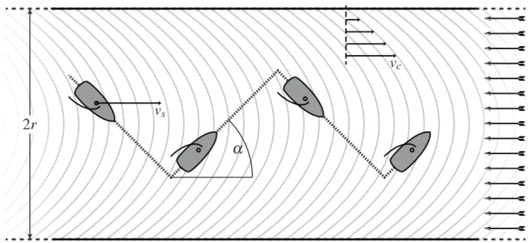
Figure 1.2: Sailing against the wind in a channel.

1.6 Sailing against the wind

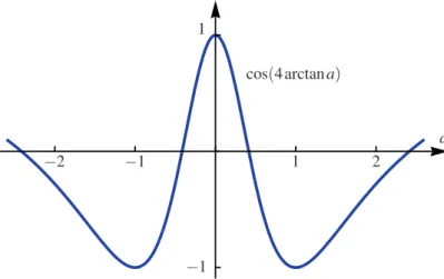
Every sailor knows how to sail against the wind by “beating”: One has to sail at an angle of approximately 45◦to the wind6, then tack (turn the bow through the wind) and finally, after the sail has caught the wind on the other side, continue again at approximately 45◦to the wind. Repeating this procedure makes the boat follow a zig-zag motion, which gives a net movement directly against the wind, see Figure 1.2. A mathematically inclined sailor might ask the question of “how often to tack”. In an idealized model we can assume that tacking costs no time and that the forward sailing speed vsof the boat depends on the angleα to the

wind as follows (at least qualitatively): vs(α) = −cos(4α),

which has maxima atα = ±45◦(in real boats, the maximum might be at a lower angle, i.e. “closer to the wind”). Assume furthermore that our sailor is sailing along a straight river with the current. Now, the current is fastest in the middle of the river and goes down to zero at the banks. In fact, a good approximation would be the formula of Poiseuille (channel) flow, which can be derived from the flow equations of fluids: At distance r from the center of the river the current’s flow speed is approximately

vc(r) := vmax ( 1− r 2 R2 ) ,

where R > 0 is half the width of the river.

(16)

If we denote by r(t) the distance of our boat from the middle of the channel at time t∈ [0,T], then the total speed (called the “velocity made good” in sailing parlance) is

v(t) := vs(arctan r′(t)) + vc(r(t)) =−cos(4arctanr′(t)) + vmax ( 1−r(t) 2 R2 ) .

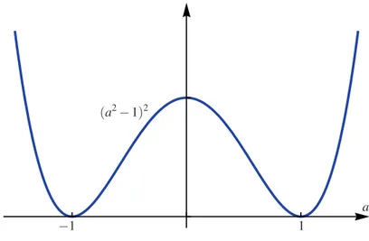
The key to understand this problem is now the fact that a7→ −cos(4arctana) has two max-ima at a =±1. We say that this function is a double-well potential.

The total forward distance traveled over the time interval [0, T ] is

∫ _T 0 v(t) dt = ∫ _T 0 −cos(4arctanr ′_{(t)) + v} max ( 1−r(t) 2 R2 ) dt.

If we also require the initial and terminal conditions r(0) = r(T ) = 0, we arrive at the optimal beating problem:

     F [r] :=∫ T 0

cos(4 arctan r′(t))− vmax ( 1−r(t) 2 R2 ) dt → min, r(0) = r(T ) = 0, |r(t)| ≤ R.

Our intuition tells us that in this idealized model, where tacking costs no time, we should be tacking as “infinitely fast” in order to stay in the middle of the river. Later, once we have advanced tools at our disposal, we will make this idea precise, see Example 5.6.

(17)

Chapter 2

Convexity

In the introduction we got a glimpse of the many applications of minimization problems in physics, technology, and economics. In this chapter we start to develop the abstract theory. Consider a minimization problem of the form

  

F [u] :=∫

Ωf (x, u(x),∇u(x)) dx → min, over all u∈ W1,p(Ω;Rm) with u|_∂_Ω= g.

Here, and throughout the course (if not otherwise stated) we will make the standard assump-tion thatΩ ⊂ Rd is a bounded Lipschitz domain, that is,Ω is open, bounded, and has a Lipschitz boundary. Furthermore, we assume 1 < p <∞, so that the integrand

f : Ω × Rm× Rm×d→ R,

is measurable in the first and continuous in the second and third arguments (hence f is a Carath´eodory integrand). For the prescribed boundary values g we assume

g∈ W1−1/p,p(∂Ω;Rm).

In this context recall that W1−1/p,p(∂Ω;Rm) is the space of all traces of functions u∈ W1,p₍_Ω;Rm_{), see Appendix A.4 for some background on Sobolev spaces. These conditions}

will be assumed from now on unless stated otherwise. Furthermore, to make the above integral finite, we assume the growth bound

| f (x,v,A)| ≤ M(1 + |v|p₊_|A|p₎ _{for some M > 0.}

Below, we will investigate the solvability and regularity properties of this minimization problem; in particular, we will take a close look at the way in which convexity properties of f in its gradient (third) argument determine whetherF is lower semicontinuous, which is the decisive attribute in the fundamental Direct Method of the Calculus of Variations.

We will also consider the partial differential equation associated with the minimization problem, the so-called Euler–Lagrange equation that is a necessary (but not sufficient) con-dition for minimizers. This leads naturally to the question of regularity of solutions. Finally,

(18)

we also treat invariances, leading to the famous Noether theorem before having a glimpse at side constraints.

Most results here are already formulated for vector-valued u, as this has many applica-tions. Some aspects, however, in particular regularity theory, are specific to scalar problems, where u is assumed to be merely real-valued.

2.1 The Direct Method

Fundamental to all of the existence theorems in this text is the conceptionally simple Direct Method1of the Calculus of Variations. Let X be a topological space2(e.g. a Banach space with the strong or weak topology) and letF : X → R ∪ {+∞} be our objective functional satisfying the following two assumptions:

(H1) Coercivity: For allΛ ∈ R, the sublevel set {x ∈ X : F [x] ≤ Λ} is sequentially rel-atively compact, that is, ifF [xj]≤ Λ for a sequence (xj)⊂ X and some Λ ∈ R, then

(xj) has a convergent subsequence.

(H2) Lower semicontinuity: For all sequences (xj)⊂ X with xj→ x it holds that

F [x] ≤ liminf

j→∞ F [xj].

Consider the abstract minimization problem

F [x] → min over all x ∈ X. (2.1)

Then, the Direct Method is the following simple strategy:

Theorem 2.1 (Direct Method). Assume thatF is both coercive and lower semicontinu-ous. Then, the abstract problem (2.1) has at least one solution, that is, there exists x_∗∈ X withF [x_∗] = min{F [x] : x ∈ X }.

Proof. Let us assume that there exists at least one x∈ X such that F [x] < +∞; otherwise, any x∈ X is a “solution” to the (degenerate) minimization problem.

To construct a minimizer we take a minimizing sequence (xj)⊂ X such that

lim

j→∞F [xj]→α := inf

{

F [x] : x ∈ X}< +∞.

Then, since convergent sequences are bounded, there existsΛ ∈ R such that F [xj]≤ Λ for

all j∈ N. Hence, by the coercivity (H1), the sequence (xj) is contained in a compact subset

1_{“Direct” refers to the fact that we construct solutions without employing a differential equation.}

2_{In fact, we only need a space together with a notion of convergence as all our arguments will involve}

sequences as opposed to more general topological tools such as nets. In all of this text we use “topology” and “convergence” interchangeably.

(19)

2.1. THE DIRECT METHOD 13

of X . Now select a subsequence, which here as in the following we do not renumber, such that

xj→ x∗∈ X.

By the lower semicontinuity (H2), we immediately conclude α ≤ F [x∗]≤ liminf

j→∞ F [xj] =α.

Thus,F [x_∗] =α and x_∗is the sought minimizer.

Example 2.2. Using the Direct Method, one can easily see that h(t) :=

{

1−t if t < 0,

t if t≥ 0, t∈ R (= X),

has minimizer t = 0, despite not even being continuous there.

Despite its nearly trivial proof, the Direct Method is very useful and flexible in applica-tions. Of course, neither coercivity nor lower semicontinuity are necessary for the existence of a minimizer. For instance, we really only needed coercivity and lower semicontinuity along a minimizing sequence, but this weaker condition is hard to check in most practical situations; however, such a refined approach can be useful in special cases.

The abstract principle of the Direct Method pushes the difficulty in proving existence of a minimizer toward establishing coercivity and lower semicontinuity. This, however, is a big advantage, since we have many tools at our disposal to establish these two hypotheses separately. In particular, for integral functionals lower semicontinuity is tightly linked to convexity properties of the integrand, as we will see throughout this course.

At this point it is crucial to observe how coercivity and lower semicontinuity interact with the topology (or, more accurately, convergence) in X : If we choose a stronger topology, i.e. one for which there are fewer convergent sequences, then it becomes easier forF to be lower semicontinuous, but harder forF to be coercive. The opposite holds if choosing a weaker topology. In the mathematical treatment of a problem we are most likely in a situation whereF and X are given by the concrete problem. We then need to find a suitable topology in which we can establish both coercivity and lower semicontinuity.

In this text, X will always be an infinite-dimensional Banach space and we have a real choice between using the strong or weak convergence. Usually, it turns out that coerciv-ity with respect to the strong convergence is false since strongly compact sets in infinite-dimensional spaces are very restricted, whereas coercivity with respect to the weak conver-gence is true under reasonable assumptions. However, whereas strong lower semicontinuity poses few challenges, lower semicontinuity with respect to weakly converging sequences is a delicate matter and we will spend considerable time on this topic.

We will always use the Direct Method in the following version:

Theorem 2.3 (Direct Method for weak convergence). Let X be a Banach space and let F : X → R ∪ {+∞}. Assume the following:

(20)

(WH1) Weak Coercivity: For allΛ ∈ R, the sublevel set

{x ∈ X : F [x] ≤ Λ} is sequentially weakly relatively compact,

that is, ifF [xj]≤ Λ for a sequence (xj)⊂ X and some Λ ∈ R, then (xj) has a weakly

convergent subsequence.

(WH2) Weak lower semicontinuity: For all sequences (xj)⊂ X with xj ⇀ x (weak

conver-gence X ) it holds that F [x] ≤ liminf

j→∞ F [xj].

Then, the minimization problem F [x] → min over all x ∈ X, has at least one solution.

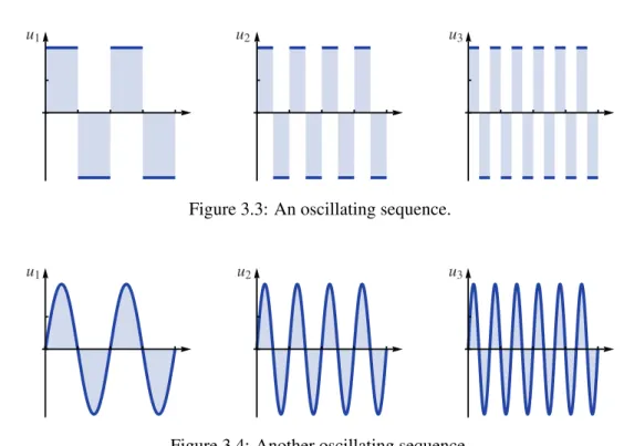
Before we move on to the more concrete theory, let us record one further remark: While it might appear as if “nature does not give us the topology” and it is up to mathematicians to “invent” a suitable one, it is remarkable that the topology that turns out to be mathematically convenient is also often physically relevant. This is for instance expressed in the following observation: The only phenomena which are present in weakly but not strongly converging sequences are oscillations and concentrations, as can be seen in the classical Vitali Con-vergence Theorem A.6. On the other hand, these phenomena very much represent physical effects, for example in crystal microstructure. Thus, the fact that we work with the weak convergence means that we have to consider microstructure (which might or might not be exhibited), a fact that we will come back to many times throughout this course.

2.2 Functionals with convex integrands

Returning to the minimization problem at the beginning of this chapter, we first consider the minimization problem for the simpler functional

F [u] :=∫

Ωf (x,∇u(x)) dx

over all u∈ W1,p(Ω;Rm) for some 1 < p <∞ to be chosen later (depending on lower growth properties of f ). The following lemma together with (2.3) allows us to conclude thatF [u] is indeed well-defined.

Lemma 2.4. Let f :Ω × RN→ R be a Carath´eodory integrand, that is, (i) x7→ f (x,A) is Lebesgue-measurable for all fixed A ∈ RN.

(21)

2.2. FUNCTIONALS WITH CONVEX INTEGRANDS 15

Then, for any Lebesgue-measurable function V : Ω → RN the composition x7→ f (x,V(x)) is Lebesgue-measurable.

We will prove this lemma via the following “Lusin-type” theorem for Carath´eodory functions:

Theorem 2.5 (Scorza Dragoni). Let f : Ω×RN→ R be Carath´eodory. Then, there exists an increasing sequence of compact sets Sk⊂ Ω (k ∈ N) with |Ω \ Sk| ↓ 0 such that f |Sk×RN

is continuous.

See Theorem 6.35 in [37] for a proof of this theorem, which is rather measure-theoretic and similar to the proof of the Lusin theorem, cf. Theorem 2.24 in [85].

Proof of Lemma 2.4. Let Sk⊂ Ω (k ∈ N) be as in the Scorza Dragoni Theorem. Set fk:=

f|_S_k_×RN and

gk(x) := fk(x,V (x)), x∈ Sk.

Then, for any open set E⊂ R, the pre-image of E under gkis the set of all x∈ Sksuch that

(x,V (x))∈ f_k−1(E). As fk is continuous, f_k−1(E) is open and from the Lebesgue

measura-bility of the product function x7→ (x,V(x)) we infer that g−1_k (E) is a Lebesgue-measurable subset of Sk. We can extend the definition of gk to all ofΩ by setting gk(x) := 0 whenever

x∈ Ω \ Sk. This function is still Lebesgue-measurable as Sk is compact, hence

measur-able. The conclusion follows from the fact that gk(x)→ f (x,V(x)) and pointwise limits of

Lebesgue-measurable functions are themselves Lebesgue-measurable.

We next investigate coercivity: Let 1 < p <∞ The most basic assumption, and the only one we want to consider here, to guarantee coercivity is the following lower growth (coercivity) bound:

µ|A|p₋_µ−1_{≤ f (x,A)} _{for all x}_{∈ Ω, A ∈ R}m×d _{and some}_{µ > 0.} _(2.2)

This coercivity also suggests the exponent p for the definition of the function spaces where we look for solutions. We further assume the upper growth bound

| f (x,A)| ≤ M(1 + |A|p₎ _{for all x}_{∈ Ω, A ∈ R}m×d _{and some M > 0,} _(2.3)

which gives finiteness ofF [u] for all u ∈ W1,p(Ω;Rm).

Proposition 2.6. If f satisfies the lower growth bound (2.2), thenF is weakly coercive on the space W1,pg (Ω;Rm) =

{

u∈ W1,p(Ω;Rm_{) : u}_|

∂Ω= g}.

Proof. We need to show that any sequence (uj)⊂ W1,pg (Ω;Rm) with

(22)

is weakly relatively compact. From (2.2) we get µ · supj ∫ Ω|∇uj| p_dx₋|Ω| µ ≤ supjF [uj] <∞,

whereby sup_j∥∇uj∥Lp <∞. By the Poincar´e–Friedrichs inequality, Theorem A.16 (I), in

conjunction with the fact that we fix the boundary values, we therefore get sup_j∥uj∥W1,p<

∞. We conclude by the fact that bounded sets in reflexive Banach spaces, like W1,p₍_Ω;Rm₎

for 1 < p <∞, are sequentially weakly relatively compact, see Theorem A.11.

Having settled the question of (weak) coercivity, we can now turn to investigate the weak lower semicontinuity.

Theorem 2.7. If A7→ f (x,A) is convex for all x ∈ Ω and f (x,A) ≥κ for some κ ∈ R (which follows in particular from (2.2)), thenF is weakly lower semicontinuous on W1,p(Ω;Rm). Proof. Step 1. We first establish that F is strongly lower semicontinuous, so let uj → u

in W1,pand∇uj→ ∇u almost everywhere (which holds after selecting a non-renumbered

subsequence, see Appendix A.2). By assumption we have f (x,∇uj(x))−κ ≥ 0.

Thus, applying Fatou’s Lemma, lim inf j→∞ ( F [uj]−κ|Ω| ) ≥ F [u] −κ|Ω|.

Thus,F [u] ≤ liminfj→∞F [uj]. Since this holds for all subsequences, it also follows for

our original sequence.

Step 2. To show weak lower semicontinuity take (uj)⊂ W1,p(Ω;Rm) with uj⇀ u. We

need to show that F [u] ≤ liminf

j→∞ F [uj] =:α. (2.4)

Taking a subsequence (not relabeled), we can in fact assume thatF [uj] converges toα.

By the Mazur Lemma A.14, we may find convex combinations vj= N( j)

∑

n= j θj,nun, where θj,n∈ [0,1] and N( j)

∑

n= j θj,n= 1,

such that vj→ u strongly. Since f (x,q) is convex,

F [vj] = ∫ Ωf ( x, N( j)

∑

n= j θj,n∇un(x) ) dx≤ N( j)

∑

n= j θj,nF [un].

Now,F [un]→α as n → ∞ and n ≥ j inside the sum. Thus,

lim inf

j→∞ F [vj]≤α = liminfj→∞ F [uj].

On the other hand, from the first step and vj→ u strongly, we have F [u] ≤ liminfj→∞F [vj].

(23)

2.2. FUNCTIONALS WITH CONVEX INTEGRANDS 17

We can summarize our findings in the following theorem:

Theorem 2.8. Let f : Ω × Rm×d be a Carath´eodory integrand such that f satisfies the lower growth bound (2.2), the upper growth bound (2.3) and is convex in its second argu-ment. Then, the associated functionalF has a minimizer over the space W1,pg (Ω;Rm).

Proof. This follows immediately from the Direct Method in Banach spaces, Theorem 2.3 together with Proposition 2.6 and Theorem 2.7.

Example 2.9. The Dirichlet integral (functional) is F [u] :=∫

Ω|∇u(x)|

2_dx, _u_{∈ W}1,2₍_Ω).

We already encountered this integral functional when considering electrostatics in Sec-tion 1.2. It is easy to see that this funcSec-tional satisfies all requirements of Theorem 2.8 and so there exists a minimizer for any prescribed boundary values g∈ W1/2,2(∂Ω). Example 2.10. In the prototypical problem of linearized elasticity from Section 1.4, we are tasked with the minimization problem

   F [u] := 1 2 ∫ Ω2µ|E u| 2₊(_{κ −}2 3µ ) |trE u|2_{− f u dx → min,} over all u∈ W1,2(Ω;R3) with u|_∂_Ω= g,

whereµ,κ > 0, f ∈ L2(Ω;R3), and g∈ W1/2,2(∂Ω;Rm). It is clear thatF has quadratic growth. Let us first consider the coercivity: For u∈ W1,2(Ω;R3) with u|_∂_Ω= g we have the following version of the L2_{-Korn inequality}

∥u∥2 W1,2≤ CK ( ∥E u∥2 L2+∥g∥2_W1/2,2 ) .

Here, CK= CK(Ω) > 0 is a constant. Let us for a simplified estimate assume thatκ −2₃µ ≥ 0

(this is not necessary, but shortens the argument). Then, also using the Young inequality, we get for anyδ > 0,

F [u] ≥µ∥E u∥2

L2− ∥ f ∥_L2∥u∥_L2 ≥µ(∥E u∥2 L2+∥g∥2_W1/2,2 ) − 1 2δ∥ f ∥ 2 L2− δ 2∥u∥ 2 L2−µ∥g∥2_W1/2,2 ≥ ( µ CK − δ 2 ) ∥u∥2 W1,2− 1 2δ∥ f ∥ 2 L2−µ∥g∥2_W1/2,2.

Choosingδ = µ/CK, we get the coercivity estimate

F [u] ≥ µ 2CK∥u∥ 2 W1,2− CK 2µ∥ f ∥ 2 L2−µ∥g∥2_W1/2,2.

Hence,F [u] controls ∥u∥_W1,2 and our functional is weakly coercive. Moreover, it is clear

that our integrand is convex in in theE u-argument (note that the trace function is linear). Hence, Theorem 2.8 yields the existence of a solution u_∗∈ W1,2₍_Ω;R3_{) to our minimization} problem of linearized elasticity.

(24)

We finish this section with the following converse to Theorem 2.7:

Proposition 2.11. LetF be an integral functional with a Carath´eodory integrand f : Ω× Rm×d _{→ R satisfying the upper growth bound (2.3). Assume furthermore that F is weakly}

lower semicontinuous on W1,p(Ω;Rm). If either m = 1 or d = 1 (the scalar case), then A7→ f (x,A) is convex for almost every x ∈ Ω.

Proof. We will not prove the full result here, since Proposition 3.27 together with Corol-lary 3.4 in the next chapter will give a stronger version (including the corresponding result for the vectorial case as well).

In the vectorial case, i.e. m̸= 1 or d ̸= 1, the necessity of convexity is far from being true and there is indeed another “canonical” condition ensuring weak lower semicontinuity, which is weaker than (ordinary) convexity; we will explore this in the next chapter.

2.3 Integrands with u-dependence

If we try to extend the results in the previous section to more general functionals F [u] :=∫

Ωf (x, u(x),∇u(x)) dx → min,

we discover that our proof strategy of using the Mazur Lemma runs into difficulties: We cannot “pull out” the convex combination inside

∫ Ωf ( x, N( j)

∑

n= j θj,nun(x), N( j)

∑

n= j θj,n∇un(x) ) dx

anymore. Nevertheless, a lower semicontinuity result analogous to the one for the scalar case turns out to be true:

Theorem 2.12. Let f :Ω × Rm× Rm×d→ R satisfy the growth bound | f (x,v,A)| ≤ M(1 + |v|p₊_|A|p₎ _{for some M > 0, 1 < p <}_∞,

and the convexity property

A7→ f (x,v,A) is convex for all (x,v) ∈ Ω × Rm. Then, the functional

F [u] :=∫

Ωf (x, u(x),∇u(x)) dx, u∈ W

1,p_(Ω;Rm_),

is weakly lower semicontinuous.

While it would be possible to give an elementary proof of this theorem here, we post-pone the verification to the next chapter. There, using more advanced and elegant techniques (blow-ups and Young measures), we will in fact establish a much more general result and see that, when viewed from the right perspective, u-dependence does not pose any additional complications.

(25)

2.4. THE EULER–LAGRANGE EQUATION 19

2.4 The Euler–Lagrange equation

In analogy to the elementary fact that the derivative of a function at its minimizers is zero, we will now derive a necessary condition for a function to be a minimizer. This condition furnishes the connection between the Calculus of Variations and PDE theory and is of great importance for computing particular solutions.

Theorem 2.13 (Euler–Lagrange equation (system)). Let f : Ω × Rm× Rm×d → R be a Carath´eodory integrand that is continuously differentiable in v and A and satisfies the growth bounds

|Dvf (x, v, A)|,|DAf (x, v, A)| ≤ M(1 + |v|p+|A|p), (x, v, A)∈ Ω × Rm× Rm×d,

for some M > 0, 1≤ p < ∞. If u_∗∈ W1,pg (Ω;Rm), where g∈ W1−1/p,p(∂Ω;Rm), minimizes

the functional F [u] :=∫

Ωf (x, u(x),∇u(x)) dx, u∈ W 1,p

g (Ω;Rm),

then u_∗ is a weak solution of the following system of PDEs, called the Euler–Lagrange equation3, { −div[DAf (x, u,∇u) ] + Dvf (x, u,∇u) = 0 in Ω, u = g on∂Ω. (2.5)

Here we used the common convention to omit the x-arguments whenever this does not cause any confusion in order to curtail the proliferation of x’s, for example in f (x, u,∇u) =

f (x, u(x),∇u(x)).

Recall that u_∗is a weak solution of (2.5) if

∫

ΩDAf (x, u∗,∇u∗) :∇ψ + Dvf (x, u∗,∇u∗)·ψ dx = 0 for allψ ∈ C∞_c(Ω;Rm), where

DAf (x, v, A) : B := lim h↓0

f (x, v, A + hB)− f (x,v,A)

h , A, B∈ R

m×d_,

is the directional derivative of f (x, v,q) at A in direction B, likewise for Dvf (x, v, A)· w.

The derivatives DAf (x, v, A) and Dvf (x, v, A) can also be represented as a matrix inRm×d

and a vector inRm, respectively, namely DAf (x, v, A) := ( ∂A_kjf (x, v, A) )j k, Dvf (x, v, A) := ( ∂vjf (x, v, A) )j .

Hence we use the notation with the Frobenius matrix vector product “:” (see the appendix) and the scalar product “·”. The boundary condition u = g on∂Ω is to be understood in the sense of trace.

(26)

Proof. For allψ ∈ C∞_c(Ω;Rm) and all h > 0 we have F [u∗]≤ F [u_∗+ hψ]

since u_∗+ hψ ∈ W1,pg (Ω;Rm) is admissible in the minimization. Thus,

0≤

∫

Ω

f (x, u_∗+ hψ,∇u_∗+ h∇ψ) − f (x,u_∗,∇u_∗)

h dx = ∫ Ω ∫ 1 0 1 h d dt [ f (x, u_∗+ thψ,∇u_∗+ th∇ψ)]dt dx = ∫ Ω ∫ 1 0 DAf (x, u∗+ thψ,∇u∗+ th∇ψ) : ∇ψ + Dvf (x, u∗+ thψ,∇u∗+ th∇ψ) · ψ dt dx.

By the growth bounds on the derivative, the integrand can be seen to have an h-uniform L1 -majorant, namely C(1 +|u_∗|p+|ψ|p+|∇u_∗|p+|∇ψ|p) and so we may apply the Lebesgue dominated convergence theorem to let h↓ 0 under the (double) integral. This yields

0≤

∫

ΩDAf (x, u∗,∇u∗) :∇ψ + Dvf (x, u∗,∇u∗)·ψ dx and we conclude by takingψ and −ψ in this inequality.

Remark 2.14. If we want to allow ψ ∈ W1,p₀ (Ω;Rm) in the weak formulation of (2.5), then we need to assume the stronger growth conditions

|Dvf (x, v, A)|,|DAf (x, v, A)| ≤ M(1 + |v|p−1+|A|p−1)

for some M > 0, 1≤ p < ∞.

Example 2.15. Coming back to the Dirichlet integral from Example 2.9, we see that the associated Euler–Lagrange equation is the Laplace equation

−∆u = 0,

where∆ :=∂_x2₁+··· +∂_x2_d is the Laplace operator. Solutions u are called harmonic func-tions. Since the Dirichlet integral is convex, all solutions of the Laplace equation are in fact minimizers. In particular, it can be seen that solutions of the Laplace equation are unique for given boundary values.

Example 2.16. In the linearized elasticity problem from Example 2.10, we may compute the Euler–Lagrange equation as

     −div [ 2µ E u + ( κ −2 3µ ) (trE u)I ] = f inΩ, u = g on∂Ω.

(27)

Sometimes, one also defines the first variationδF [u] of F at u ∈ W1,p(Ω;Rm) as the linear map

δF [u]: W1,p

0 (Ω;Rm)→ R through (whenever this exists)

δF [u][ψ] := lim h↓0 F [u + hψ] − F [u] h , ψ ∈ W 1,p 0 (Ω;R m_).

Then, the assertion of the previous theorem can equivalently be formulated as δF [u∗] = 0 if u∗minimizesF over W1,pg (Ω;Rm).

Of course, this condition is only necessary for u to be a minimizer. Indeed, any solution of the Euler–Lagrange equation is called a critical point ofF , which could be a minimizer, maximizer, or saddle point.

One crucial consequence of the results in this section is that we can use all available PDE methods to study minimizers. Immediately, one can ask about the type of PDE we are dealing with. In this respect we have the following result:

Proposition 2.17. Let f be twice continuously differentiable in v and A. Also let A7→ f (x, v, A) be convex for all (x, v)∈ Ω×Rm. Then, the Euler–Lagrange equation is an elliptic PDE, that is,

0≤ D2_Af (x, v, A)[B, B] := d 2 dt2f (x, v, A + tB) t=0

for all x∈ Ω, v ∈ Rm, and A, B∈ Rm×d.

This proposition is not difficult to establish and just needs a bit of notation; we omit the proof.

One main use of the Euler–Lagrange equation is to find concrete solutions of variational problems:

Example 2.18. Recall the optimal saving problem from Section 1.5,    F [S] :=∫ T 0 −ln(w +ρS(t) − ˙S(t)) dt → min, S(0) = 0, S(T ) = ST≥ 0.

The Euler–Lagrange equation is −d dt [ 1 w +ρS(t) − ˙S(t) ] =− ρ w +ρS(t) − ˙S(t), which resolves to ρ ˙S(t) − ¨S(t) w +ρS(t) − ˙S(t)=ρ.

(28)

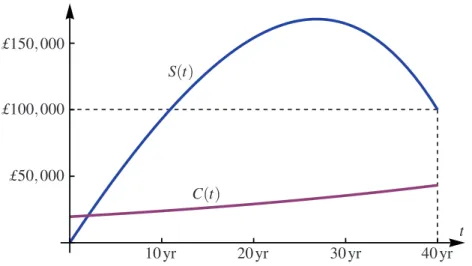
Figure 2.1: The solution to the optimal saving problem.

With the consumption rate C(t) := w +ρS(t) − ˙S(t), this is equivalent to ˙

C(t) C(t)=ρ,

and so, if C(0) = C0(to be determined later), w +ρS(t) − ˙S(t) = C(t) = eρtC0.

This differential equation for S(t) can be solved, for example via the Duhamel formula, which yields S(t) = eρt· 0 + ∫ t 0 eρ(t−s)(w− eρsC0) ds =e ρt_{− 1} ρ w−teρtC0.

and C0 can now be chosen to satisfy the terminal condition S(T ) = ST, in fact, C0= (1− e−ρT)w/(ρT) − e−ρTST/T .

Since C7→ −lnC is convex, we know that S(t) as above is a minimizer of our problem. In Figure 2.1 we see the optimal savings strategy for a worker earning a (constant) salary of w = £30, 000 per year and having a savings goal of ST= £100, 000. The worker has to

save for approximately 27 years, reaching savings of just over £168, 000, and then starts withdrawing his savings ( ˙S(t) < 0) for the last 13 years. The worker’s consumption C(t) = eρtC0 goes up continuously during the whole working life, making him/her (materially) happy.

(29)

Example 2.19. For functions u = u(t, x) : R × Rd→ R, consider the action functional A [u] :=1 2 ∫ R×Rd−|∂tu| 2₊_|∇ xu|2d(t, x),

where∇xu is the gradient of u with respect to x∈ Rd. This functional should be interpreted

as the usual Dirichlet integral, see Example 2.9, where, however, we use the Lorentz metric. Then, the Euler–Lagrange equation is the wave equation

∂2

t u− ∆u = 0.

Notice thatA is not convex and consequently the wave equation is hyperbolic instead of elliptic.

It is an important question whether a weak solution of the Euler–Lagrange equation (2.5) is also a strong solution, that is, whether u∈ W2,2(Ω;Rm) and

{

−div[DAf (x, u(x),∇u(x))

]

+ Dvf (x, u(x),∇u(x)) = 0 for a.e. x ∈ Ω,

u = g on∂Ω. (2.6)

If u∈ C2(Ω;Rm₎_{∩ C(Ω;R}m_{) satisfies this PDE for every x}_{∈ Ω, then we call u a classical}

solution.

Multiplying (2.6) by a test functionψ ∈ C∞_c(Ω;Rm), integrating overΩ, and using the Gauss–Green Theorem, it follows that any solution of (2.6) also solves (2.5). The converse is also true whenever u is sufficiently regular:

Proposition 2.20. Let the integrand f be twice continuously differentiable and let u∈ W2,2₍_Ω;Rm_{) be a weak solution of the Euler–Lagrange equation (2.5). Then, u solves the}

Euler–Lagrange equation (2.6) in the strong sense. Proof. If u∈ W2,2(Ω;Rm) is a weak solution, then

∫

ΩDAf (x, u,∇u) : ∇ψ + Dvf (x, u,∇u) ·ψ dx = 0

for allψ ∈ C∞_c(Ω;Rm_{). Integration by parts (more precisely, the Gauss–Green Theorem)}

gives ∫ Ω { −div[DAf (x, u,∇u) ] + Dvf (x, u,∇u) } ·ψ dx = 0,

again for allψ as before. We conclude using the following important lemma.

Lemma 2.21 (Fundamental lemma of the Calculus of Variations). LetΩ ⊂ Rdbe open. If g∈ L1(Ω) satisfies

∫

Ωgψ dx = 0 for allψ ∈ C ∞

c(Ω),

(30)

Proof. We can assume thatΩ is bounded by considering subdomains if necessary. Also, let g be extended by zero to all ofRd. Fixε > 0 and let (ρ_δ)_δ ⊂ C∞_c(B(0,δ)) be a family of mollifying kernels, see Appendix A.2 for details. Then, sinceρ_δ⋆ g→ g in L1, we may find h∈ (L1∩ C∞)(Rd) with

∥g − h∥L1 ≤ε

4 and ∥h∥∞<∞.

Setφ(x) := h(x)/|h(x)| for h(x) ̸= 0 and φ(x) := 0 for h(x) = 0, so that hφ = |h|. Then take ψ = ρ_δ¯⋆φ ∈ (L1∩ C∞)(Rd) with

∥φ − ψ∥L1 ≤ ε

2∥h∥_∞.

Since|ψ| ≤ 1 (this follows from the convolution formula), ∥g∥L1≤ ∥g − h∥_L1+ ∫ Ωhφ dx ≤ ∥g − h∥L1+ ∫ Ωh(φ − ψ) + (h − g)ψ + gψ dx ≤ 2∥g − h∥L1+∥h∥∞· ∥φ − ψ∥_L1+ 0 ≤ε. We conclude by lettingε ↓ 0.

2.5 Regularity of minimizers

As we saw at the end of the last section, whether a weak solution of the Euler–Lagrange equation is also a strong or even classical solution, depends on its regularity, that is, on the amount of differentiability. More generally, one would like to know how much regularity we can expect from solutions of a variational problem. Such a question also was the content of David Hilbert’s 19th problem [47]:

Does every Lagrangian partial differential equation of a regular variational problem have the property of exclusively admitting analytic integrals?4

In modern language, Hilbert asked whether “regular” variational problems (defined below) admit only analytic solutions, i.e. ones that have a local power series representation.

In this section, we will prove some basic regularity assertions, but we will only sketch the solution of Hilbert’s 19th problem, as the techniques needed are quite involved. We re-mark from the outset that regularity results are very sensitive to the dimensions involved, in particular the behavior of the scalar case (m = 1) and the vector case (m > 1) is fundamen-tally different. We also only consider the quadratic (p = 2) case for reasons of simplicity.

4_{The German original asks “ob jede Lagrangesche partielle Differentialgleichung eines regul¨aren}

(31)

2.5. REGULARITY OF MINIMIZERS 25

In the spirit of Hilbert’s 19th problem, call F [u] :=∫

Ωf (∇u(x)) dx, u∈ W

1,2₍_Ω;Rm_),

a regular variational integral if f ∈ C2(Rm×d) and there are constants 0 <µ ≤ M with µ|B|2_{≤ D}2

Af (A)[B, B]≤ M|B|2 for all A, B∈ Rm×d.

In this context, D2_Af (A)[B1, B2] = d dt d dsf (A + sB1+ tB2) s,t=0 for all A, B1, B2∈ Rm×d,

which is a bilinear form. Clearly, regular variational problems are convex. In fact, inte-grands f that satisfy the above lower boundµ|B|2≤ D2_Af (A)[B, B] are called strongly con-vex. For example, the Dirichlet integral from Example 2.9 is regular. Also, the following Cauchy–Schwarz-type estimate can be shown:

D2_Af (A)[B1, B2] ≤M|B1||B2|. (2.7)

The basic regularity theorem is the following:

Theorem 2.22 (W2,2_loc-regularity). Let F be a regular variational integral. Then, for any minimizer u∈ W1,2(Ω;Rm) ofF , it holds that u ∈ W2,2_loc(Ω;Rm). Moreover, for any B(x0, 3r)⊂ Ω (x0∈ Ω, r > 0) the Caccioppoli inequality

∫ B(x0,r) |∇2_u(x)_|2_dx_≤ ( 2M µ )2∫ B(x0,3r) |∇u(x) − [∇u]B(x0,3r)| 2 r2 dx (2.8)

holds, where [∇u]B(x0,3r) := − ∫

B(x0,3r)∇u dx. Consequently, the Euler–Lagrange equation

holds strongly,

−divD f (∇u) = 0, a.e. inΩ.

For the proof we employ the difference quotient method, which is fundamental in regu-larity theory. Let u : Ω → Rm, x∈ Ω, k ∈ {1,...,d}, and h ∈ R. Then, define the difference quotients

Dh_ku(x) := u(x + hek)− u(x)

h , D

h_{u := (D}h

1u, . . . , Dhdu),

where{e1, . . . , ed} is the standard basis of Rd. The key is the following characterization of

Sobolev spaces in terms of difference quotients:

Lemma 2.23. Let 1 < p <∞, D ⊂⊂ Ω ⊂ Rdbe open, and u∈ Lp(Ω;Rm_).

(I) If u∈ W1,p(Ω;Rm), then ∥Dh

(32)

(II) If for some 0 <δ < dist(D,∂Ω) it holds that ∥Dh

ku∥Lp_(D)≤ C for all k∈ {1,...,d} and all |h| <δ,

then u∈ W1,p_loc(Ω;Rm_{) and}_∥_∂

ku∥Lp_(D)≤ C for all k ∈ {1,...,d}.

Proof. For (I), assume first that u∈ (Lp∩ C1)(Ω;Rm). In this case, by the Fundamental Theorem of Calculus, at x∈ Ω it holds that

Dh_ku(x) =1 h ∫ ₁ 0 d dtu(x + thek) dt = ∫ ₁ 0 ∂k u(x + thek) dt. Thus, ∫ D|D h ku|pdx≤ ∫ Ω|∂ku| p_dx,

from which the assertion follows. The general case follows from the density of (Lp∩ C1)(Ω;Rm_{) in L}p₍_Ω;Rm_).

For (II), we observe that for fixed k∈ {1,...,d} by assumption (Dh_ku)0<h<δis uniformly Lp-bounded. Thus, for an arbitrary fixed sequence of h’s tending to zero, there exists a subsequence hj↓ 0 with

Dhj

k u ⇀ vk in L p

for some vk ∈ Lp(Ω;Rm). Let ψ ∈ C∞c(Ω;Rm). Using an “integration-by-parts” rule for

difference quotients, which is elementary to check, we get

∫ D vk·ψ dx = lim j→∞ ∫ D Dh_kju·ψ dx = − lim j→∞ ∫ D u· D−h_k jψ dx = − ∫ D u·∂kψ dx. Thus, u∈ W1,p(D;Rm_{) and v}

k=∂ku. The norm estimate follows from the lower

semicon-tinuity of the norm under weak convergence.

Proof of Theorem 2.22. The idea is to emulate the a-priori non-existent second derivatives using difference quotients and to derive estimates which allow one to conclude that these difference quotients are in L2. Then we can conclude by the preceding lemma.

Let u∈ W1,2(Ω;Rm) be a minimizer ofF . By Theorem 2.13, 0 =

∫

ΩD f (∇u) : ∇ψ dx (2.9)

holds for allψ ∈ C∞_c(Ω;Rm), and then by density also for allψ ∈ W1,2(Ω;Rm). Here we have used the notation D f (A) : B for the directional derivative of f at A in direction B. Fix a ball B(x0, 3r)⊂ Ω and take a Lipschitz cut-off functionρ ∈ W1,∞(Ω) such that

1B(x0,r)≤ρ ≤ 1B(x0,2r) and |∇ρ| ≤

1 r.

(33)

2.5. REGULARITY OF MINIMIZERS 27

Then, for any k = 1, . . . , d and|h| < r, we let ψ := D−hk [ ρ2_Dh k(u− a) ] ∈ W1,2₍_Ω;Rm_),

where a is an affine function to be chosen later. We may plugψ into (2.9) to get 0 = ∫ ΩD h k(D f (∇u)) : [ ρ2_Dh k∇u + Dhk(u− a) ⊗ ∇(ρ2) ] dx. (2.10)

Here, we used the “integration-by-parts” formula for difference quotients, which is easy to check (also recall a⊗ b := abT).

Next, we estimate, using the assumptions on f , µ|Dh

k∇u|2≤

∫ 1 0

D2f (∇u +thDh_k∇u)[Dh_k∇u,Dh_k∇u] dt =1 hD f (∇u +thD h k∇u) : Dhk∇u 1 t=0 = Dh_k(D f (∇u)) : Dh_k∇u.

From the preceding lemma (both parts), (2.7), and the fact|a ⊗ b| = |a| · |b| for our norms, we get

Dh_k(D f (∇u)) :[Dh_k(u− a) ⊗ ∇(ρ2)] ≤ D2f (∇u)[Dh_k(u− a) ⊗ ∇(ρ2),∂k∇u]

≤ 2M ·ρ · |Dh

k(u− a)| · |∇ρ| · |Dhk∇u|.

Using the last two estimates, (2.10), and the integration-by-parts formula for difference quotients again, µ∫ Ω|D h k∇u|2ρ2dx≤ ∫ ΩD h k(D f (∇u)) : [ρ2Dhk∇u] dx =− ∫ ΩD h k(D f (∇u)) : [ Dh_k(u− a) ⊗ ∇(ρ2)]dx ≤ 2M∫ Ωρ · |D h k∇u| · |Dhk(u− a)| · |∇ρ| dx.

Absorbing the first term in the left hand side and using the properties ofρ,

∫ B(x0,r) |Dh k∇u|2dx≤ ( 2M µ )2∫ B(x0,2r) |Dh k(u− a)|2 r2 dx.

Now invoke the difference-quotient lemma, part (I), to arrive at

∫ B(x0,r) |Dh k∇u|2dx≤ ( 2M µ )2∫ B(x0,3r) |∂k(u− a)|2 r2 dx.

Applying the lemma again, this time part (II), we get u∈ W2,2_(B(x

0, r);Rm). The Cacciop-poli inequality (2.8) follows once we take∇a := [∇u]B(x0,3r).

(34)

With the W2,2_loc-regularity result at hand, we may use ψ = ∂kψ, k = 1,...,d, as test˜

function in the weak formulation of the Euler–Lagrange equation −div[D f (∇u)] = 0 to conclude that

−div[D2f (∇u) : ∇(∂ku)

]

= 0 (2.11)

holds in the weak sense. Indeed, 0 =− ∫ Ωdiv D f (∇u) ·∂kψ dx = ∫ Ωdiv [ D2f (∇u) : ∇(∂ku) ] ·ψ dx

for allψ ∈ C∞_c(Ω;Rm). In the special case that f is quadratic, D2f is constant and the above PDE has the same structure (with∂ku as unknown function) as the original Euler–Lagrange

equation. Thus it is itself an Euler–Lagrange equation and we can bootstrap the regularity theorem to get u∈ Wk,2_loc(Ω;Rm) for all k∈ N, hence k ∈ C∞(Ω;Rm).

Example 2.24. For a minimizer u∈ W1,2(Ω) of the Dirichlet integral as in Example 2.9, the theory presented here immediately gives u∈ C∞(Ω).

Example 2.25. Similarly, for minimizers u∈ W1,2(Ω;R3_{) to the problem of linearized} elasticity from Section 1.4 and Example 2.10, we also get u∈ C∞(Ω;R3). The reasoning has to be slightly adjusted, however, to take care of the fact that we are dealing with E u instead of∇u.

In the general case, however, our Euler–Lagrange equation is nonlinear and the above bootstrapping procedure fails. In particular, this includes the problem posed in Hilbert’s 19th problem, which was only solved, in the scalar case m = 1, by Ennio De Giorgi in 1957 [28] and, using different methods, by John Nash in 1958 [78]. After the proof was improved by J¨urgen Moser in 1960/1961 [71, 72], the results are now subsumed in the De Giorgi–Nash–Moser theory.

The current standard solution (based on De Giorgi’s approach) is based on the De Giorgi regularity theoremand the classical Schauder estimates, which establish H¨older regular-ity of weak solutions of a PDE.

Theorem 2.26 (De Giorgi regularity theorem). Let the function A : Ω → Rd×d be mea-surable, symmetric, i.e. A(x) = A(x)T for x∈ Ω, and satisfy the ellipticity and boundedness estimates

µ|v|2_{≤ v}T_A(x)v_{≤ M|v|}2_, _x_{∈ Ω,v ∈ R}d_, _(2.12)

for constants 0 <µ ≤ M. If u ∈ W1,2(Ω) is a weak solution of

−div[A∇u] = 0, (2.13)

then u∈ C0,α0