Quantum Theory A Complete Introduction pdf - Web Education

Quantum

mechanics

Alexandre Zagoskin is a Reader in Quantum

Physics at Loughborough University and a

Fellow of The Institute of Physics.

He received his Master’s degree in physics

from Kharkov University (Soviet Union),

and his PhD in physics from the Institute for

Low Temperature Physics and Engineering

(FTINT), also in Kharkov. He has worked at

FTINT, Chalmers University of Technology

(Sweden), the University of British Columbia

(Canada) and the RIKEN Institute (Japan).

In 1999, when in Canada, he co-founded the

company D-Wave Systems with the aim of

developing commercial quantum computers,

and was its Chief Scientist and VP of

Research until 2005.

He has published two books: Quantum

Theory of Many-Body Systems (Springer,

1998, 2014) and Quantum Engineering

(Cambridge University Press, 2011).

He and his colleagues are now working

on the development of quantum

engineering – the theory, design, fabrication

and characterization of quantum coherent

artificial structures.

Quantum

mechanics

A Complete Introduction

Alexandre Zagoskin

First published in Great Britain in 2015 by John Murray Learning. An Hachette UK company.

First published in US in 2015 by Quercus Copyright © Alexandre Zagoskin 2015

The right of Alexandre Zagoskin to be identified as the Author of the Work has been asserted by him in accordance with the Copyright, Designs and Patents Act 1988.

Database right Hodder & Stoughton (makers)

The Teach Yourself name is a registered trademark of Hachette UK. All rights reserved. No part of this publication may be reproduced, stored in a retrieval system or transmitted in any form or by any means, electronic, mechanical, photocopying, recording or otherwise, without the prior written permission of the publisher, or as expressly permitted by law, or under terms agreed with the appropriate reprographic rights organization. Enquiries concerning reproduction outside the scope of the above should be sent to the Rights Department, John Murray Learning, at the address below.

You must not circulate this book in any other binding or cover and you must impose this same condition on any acquirer.

British Library Cataloguing in Publication Data: a catalogue record for this title is available from the British Library.

Library of Congress Catalog Card Number: on file. 1

The publisher has used its best endeavours to ensure that any website addresses referred to in this book are correct and active at the time of going to press. However, the publisher and the author have no responsibility for the websites and can make no guarantee that a site will remain live or that the content will remain relevant, decent or appropriate.

The publisher has made every effort to mark as such all words which it believes to be trademarks. The publisher should also like to make it clear that the presence of a word in the book, whether marked or unmarked, in no way affects its legal status as a trademark.

Every reasonable effort has been made by the publisher to trace the copyright holders of material in this book. Any errors or omissions should be notified in writing to the publisher, who will endeavour to rectify the situation for any reprints and future editions.

Cover image © Shutterstock.com Typeset by Cenveo® _{Publisher Services.}

Printed and bound in Great Britain by CPI Group (UK) Ltd., Croydon, CR0 4YY.

John Murray Learning policy is to use papers that are natural, renewable and recyclable products and made from wood grown in sustainable forests. The logging and manufacturing processes are expected to conform to the environmental regulations of the country of origin.

Carmelite House 50 Victoria Embankment London EC4Y 0DZ www.hodder.co.uk

Contents

acknowledgements

x

introduction

xi

A fair warning

1 Familiar physics in strange spaces

1

Particles, coordinates, vectors and trajectories

Velocity, acceleration, derivatives and differential equations Phase space

Harmonic oscillator, phase trajectories, energy conservation and action

Hamilton, Hamiltonian, Hamilton’s equations and state vectors

Generalized coordinates, canonical momenta, and configuration space

Statistical mechanics, statistical ensemble and probability distribution function

Liouville equation*

2 Less familiar physics in stranger spaces

34

Quantum oscillator and adiabatic invariants

Action quantization, phase space and the uncertainty principle Zero-point energy and complex numbers

State vector and Hilbert space

Operators, commutators, observables and expectation values Eigenstates, eigenvalues, intrinsic randomness of

Nature and Born’s rule

Quantization and Heisenberg uncertainty relations

3 equations of quantum mechanics

66

Poisson brackets, Heisenberg equations of motion and the Hamiltonian

Matrices and matrix elements of operators Schrödinger equation and wave function Quantum propagation

A particle in a box and on a ring: energy and momentum quantization

Quantum superposition principle

Quantum statistical mechanics, quantum ensembles and density matrix*

4 Qubits and pieces

96

Qubits and other two-level quantum systems Qubit’s state vector, Hilbert space, Bloch vector and Bloch sphere

Qubit Hamiltonian and Schrödinger equation Energy eigenstates and quantum beats

Bloch equation, quantum beats (revisited) and qubit control Qubit observables, Pauli matrices and expectation values Qubit density matrix, von Neumann and Bloch

equations and NMR* Vintage charge qubits

5 Observing the observables

134

Measurement, projection postulate and Born’s rule (revisited) The ‘collapse of the wave function’, measurement

problem and quantum-classical transition Observing a charge qubit

Bloch vector and density matrix; Bloch equations (revisited); dephasing; and weak continuous measurement*

Measurements and Heisenberg uncertainty relations: Heisenberg microscope

Standard quantum limit

Quantum non-demolition (QND) measurements and energy-time uncertainty relation

Quantum Zeno paradox

6 strange and unusual

165

Quantum tunnelling: α-decay

Quantum tunnelling: scanning tunnelling microscope

Waves like particles: photoelectric effect and the single-photon double slit experiment

Particles like waves: diffraction and interference of massive particles; de Broglie wavelength

7 the game of numbers

191

Electron in an atom

Electrons in an atom and Mendeleev periodic table Pauli exclusion principle, fermions and bosons, and spin Quantum many-body systems, Fock states, Fock space and creation and annihilation operators

Quantum oscillator, Heisenberg equations and energy quanta* Quantum fields and second quantization

8 the virtual reality

221

Electrons in a jellium, charge screening, electron gas and Fermi–Dirac distribution

Electrons in a crystal: quasiparticles*

Electrons in a crystal: Bloch functions; quasimomentum; Brillouin zones; energy bands; and Fermi surface* Quasiparticles and Green’s functions

Perturbation theory

Feynman diagrams and virtual particles

Summing Feynman diagrams and charge screening Dressing the quasiparticles

9 the path of extremal action

254

Variational approach to classical mechanics Variational approach to quantum mechanics Feynman’s path integrals

Charged quantum particles in an electromagnetic field, path integrals, the Aharonov–Bohm effect and the Berry phase*

10 Order! Order!

281

Classical magnets, second order phase transitions and the order parameter

Landau’s theory of second order phase transitions and spontaneous symmetry breaking

Superconductors, superconducting phase transition and the superconducting order parameter

BCS theory, Bose–Einstein condensate, Cooper pairs and the superconducting energy gap

Josephson effect*

11 curiouser and curiouser

311

Einstein-Podolsky-Rosen paradox

Entanglement and faster-than-light communications Spooks acting at a distance, no-cloning

and quantum tomography

Schrödinger’s cat and Wigner’s friend Bell’s inequality*

12 schrödinger’s elephants and quantum

slide rules

339

The need and promise of quantum computers Digital computers, circuits and gates Quantum gates

Quantum parallelism and the Deutsch algorithm*

The Shor algorithm, code-breaking and the promise of an exponential speed-up

Schrödinger’s elephants, quantum error correction and DiVincenzo criteria

Quantum slide rules: adiabatic quantum computing and quantum optimizers

13 history and philosophy

374

Sturm und Drang: the old quantum theory

When all roads led to Copenhagen: creation of quantum mechanics

What the FAPP?

‘It was a warm summer evening in ancient Greece’ The proof of the pudding

The final spell

Fact-check answers

393

taking it further

395

Figure credits

397

How to use this book

This Complete Introduction from Teach Yourself® includes a number of special boxed features, which have been developed to help you understand the subject more quickly and remember it more effectively. Throughout the book, you will find these indicated by the following icons

The book includes concise quotes from other key sources. These will be useful for helping you understand different viewpoints on the subject, and they are fully referenced so that you can include them in essays if you are unable to get your hands on the source.

The case study is a more in-depth introduction to a particular example. There is at least one in most chapters, and they should provide good material for essays and class discussions.

The key ideas are highlighted throughout the book. If you only have half an hour to go before your exam, scanning through these would be a very good way of spending your time.

The spotlight boxes give you some light-hearted additional information that will liven up your learning.

The fact-check questions at the end of each chapter are designed to help you ensure you have taken in the most important concepts from the chapter. If you find you are consistently getting several answers wrong, it may be worth trying to read more slowly, or taking notes as you go.

The dig deeper boxes give you ways to explore topics in greater depth than is possible in this introductory-level book.

Acknowledgements

I am grateful to my friends, colleagues and students, discussions with whom helped me better understand many topics covered in this book; and to D. Palchun, R. Plehhov and E. Zagoskina, who agreed to be test subjects for some parts of the manuscript and lived to tell me about the experience.

Introduction

A fair warning

The first thing a student of magic learns is that there are books about magic and books of magic. And the second thing he learns is that a perfectly respectable example of the former may be had for two or three guineas at a good bookseller, and that the value of the latter is above rubies.

Susanna Clarke, Jonathan Strange & Mr Norrell

This book will help you teach yourself about quantum mechanics, which is not quite the same as teaching yourself quantum mechanics. Here is the difference.

To learn quantum mechanics means being able to do something with quantum mechanics as a matter of course (solving equations, mostly. If you are an experimentalist, this also entails conducting experiments, the planning and analysis of which require solving equations), and to have been doing this long enough to acquire a certain intuition about these equations and experiments – and therefore, about quantum mechanics. At the very least, one would have to go through a good undergraduate textbook on quantum mechanics and solve all the problems (which means also going through a couple of textbooks on mathematics and solving the problems from them too), and discuss all the questions you may have with somebody who already has the above-mentioned intuition. In other words, to take a regular introductory course of quantum mechanics at a university, and this is not always an option. And anyway, you may not be planning to become a professional physicist (which is a pity).

You can instead learn about quantum mechanics. This is a book written exactly for this purpose – to help you teach yourself about quantum mechanics. This means that in the end you will not become a practising magician, that is, physicist – but hopefully you will have a better understanding of what physicists do and think when they do research in quantum

mechanics, and what this research tells us about the world we live in. Besides, much of our technology uses quantum mechanical effects routinely (like lasers and semiconductor microchips, which were produced by the ‘first quantum revolution’ back in the 20th century), and if the current trends hold, we will be soon enough playing with the technological results of the ‘second quantum revolution’, using even more subtle and bizarre quantum effects. It is therefore wise to be prepared. As a bonus, you will learn about quite a lot of things that are not taught in introductory quantum mechanics courses to physics undergraduates.

This book contains quite a number of equations (though much less than a book of quantum mechanics would), so brushing up your school maths would be a good idea. I have tried to introduce all the new mathematical things, and some things you may already know. Still, this is just a book about quantum mechanics. So why equations?

Quantum mechanics describes our world with an unbelievable precision. But the scale of phenomena, where this description primarily applies, is so far removed from our everyday experience that our human intuition and language, however rich, are totally inadequate for the task of expressing quantum mechanics directly. In such straits it was common to use poetry with its allusions, allegories and similes. This is indeed the only way one can write about quantum mechanics using only words – even if the poetry lacks rhymes and rhythm. This is a nice and often inspiring way of doing things, but poetry is too imprecise, too emotional and too individual.

It is therefore desirable to use the language in which quantum mechanics can be expressed: mathematics, a language more remote from our common speech than any Elvish dialect. Fortunately, this is also the language in which all physics is most naturally expressed, and it applies to such areas – like mechanics – where we do have an inborn and daily trained intuition. I did therefore try to relate the one to the other – you will be the judge of how well this approach succeeded.1

1

Familiar physics in

strange spaces

mechanics may seem intimidatingly impenetrable. It is full of commutators, operators, state vectors, Hilbert spaces and other mathematical horrors. At any rate quantum physics seems totally different from the clarity and simplicity of Newtonian mechanics, where footballs, cars, satellites, stars, planets, barstools, bees, birds and butterflies move along well-defined trajectories, accelerate or decelerate when acted upon by forces, and always have a definite position and velocity. All this can be described by the simple mathematical laws discovered by Sir Isaac Newton and taught at school – or just intuitively comprehended based on our everyday experience. Quantum mechanics, on the contrary, is best left to somebody else.

Philosophy is written in that great book which ever lies before our eyes – I mean the universe – but we cannot understand it if we do not first learn the language and grasp the symbols, in which it is written. This book is written in the mathematical language, and the symbols are triangles, circles and other geometrical figures, without whose help it is impossible to comprehend a single word of it; without which one wanders in vain through a dark labyrinth.

Galileo Galilei (1564–1642)

Spotlight: Rene Descartes (1596–1650)

Actually, this impression is false. We are not saying that quantum mechanics does not differ from classical mechanics – of course it does, and it indeed presents a counterintuitive, puzzling, very beautiful and very precise view of the known Universe. But to see these differences in the proper light, it is necessary first to cast a better look at the structure of classical mechanics and realize – to our surprise – that in many important respects it is very similar to quantum mechanics.

Key idea: coordinate transformation

Switching between different coordinate systems is called coordinate transformation. Here is a simple example. Suppose a point A has coordinates (x,y,z). Let us now introduce a new coordinate system (O’x’y’z’) with the origin in the point O’ with coordinates (X,Y,Z).

z z´ O´ O y´ x´ x y

As you can see from the diagram, the coordinates (x’,y’,z’) of the same point A in the new system are given by

x' _{= x − X, y' = y − Y, z' = z − Z.} Any coordinate transformation can be written as:

(x’,y’,z’) _{= Λ (x,y,z).}

Here Λ is shorthand for an explicitly known set of operations one must perform with the set of coordinates in the original system, in order to obtain the coordinates of the same point in the new one. Mathematically, this means that Λ is an operator – the first scary word is demystified.

Of course, to see this one has to venture beyond Newtonian dynamics, but this exercise does not require any extraordinary effort. We will however need some mathematics. The reason being that mathematics is a very concise and precise language, specially developed over the centuries to describe complex natural phenomena and to make precise and verifiable statements. Physics in this respect is not unlike Shakespeare’s works: in order to enjoy the play and understand what it is about, you should know the language, but you do not need to know the meaning of every single word or be good at writing sonnets.

Much of what will be required for the following you may have already studied at school (but perhaps looked at from a different angle) – look at the boxes for reminders, explanations and other useful information.

Particles, coordinates, vectors

and trajectories

Consider a material point or a particle – the simplest object of Newtonian dynamics. Visualize this as an infinitesimally small, massive, structureless object. For example, a good model for this would be a planet orbiting the Sun but not too close to it, or the bob of a pendulum. Since the times of Descartes, we know that the position of a point in space can be completely determined by a set of three numbers – its Cartesian coordinates (x,y,z), which give its distances from the origin O along the three mutually orthogonal (that is, at right angles to each other) coordinate axes Ox, Oy, Oz (Figure 1.1). These axes and their common origin O (the reference point) form a Cartesian coordinate system. Just look at a corner of your room, and you will see, as did Descartes four centuries ago, the origin and the three coordinate axes meeting there.2

Spotlight: at a tangent

According to classical mechanics, ‘to fly at a tangent’ actually means ‘to keep moving in the same direction as before’, and not ‘to start on something completely different’!

Key idea: Functions

A quantity f, which depends on some variable x, is called a function of x and is usually denoted by f(x). Thus, the radius vector is a function of x, y and z.

2 If you happen to live in a round, spherical or even crooked house, there exist appropriate coordinate systems too – but they would lead us too far

Spotlight: Looking for treasure

If you wish, you can treat a radius vector as a set of instructions on a treasure map. For example, from the old oak tree, go x feet east, then y feet north, then dig a hole (-z) feet deep (or climb z feet up a cliff). N S E W 15 0 50 Dig here 7↓

There can be any number of such coordinate systems, with different reference points and different directions of the axes, but once the coordinates (x,y,z) of a point are known in one coordinate system, they are readily found in any other system. We can also determine the position of our point by a radius vector r – a straight arrow connecting it with the reference point O (Figure 1.1). Of course, both descriptions are equivalent, and we can write simply

r = (x, y, z),

that is, a vector is a set of three Cartesian coordinates (which are called its Cartesian components and must be properly transformed if we decide to switch to another coordinate system). We can easily add or subtract two vectors by adding or subtracting their corresponding components. For example, if our material point moved the distance Δx along the axis Ox, Δy along Oy, and Δz along Oz, its new position will be given by a radius vector (Figure 1.2):

r’ _{= (x + Δx, y + Δy, z + Δz) ≡ r + Δr,} where the vector Δr = (Δx, Δy, Δz) is the displacement.

(The sign of equivalence ‘≡’ means ‘the same as’, and by Δa one customarily denotes a change in the variable a.)

If we now add to our coordinate system a clock, which

measures time t, it becomes a reference frame. The position of a point will now depend on time,

r(t) ≡ (x(t), y(t), z(t)),

and as the time passes, the end of the radius vector traces a line in space – the trajectory of the point (Figure 1.1).

z

y O

x

Figure 1.1 cartesian coordinates, radius vector and a trajectory.

Velocity, acceleration, derivatives

and differential equations

Key idea: calculus

The calculus, including the concept of differentiation (finding derivatives), was independently developed by Newton and Leibniz. The nomenclature and notation proposed by Leibniz (in particular, the term ‘derivative’ and the symbol dx_dt for it) turned out to be more convenient, although sometimes Newtonian notation is also used:

x dx

dt ≡

Key idea: Derivative

The derivative _dxdf is the mathematically rigorous expression for the rate of change of a function f (x) as the variable x changes. For example, the incline of a slope is given by the derivative of height with respect to the horizontal displacement:

dh x dx tanα = ( ) x h α

The Leibniz’s notation for the derivative reflects the fact that it is a limit of the ratio of a vanishingly small change Δf, to a vanishingly small change Δx.

Now we can define the velocity. Intuitively, the velocity tells us how fast something changes its position in space. Let the point move for a short time interval Δt from the position r(t) to r(t _{+ Δt) (Figure 1.2):}

r (t + Δt) = r (t) + Δr.

Its average velocity is then vav= ∆∆r_t . Now, let us make the time interval Δt smaller and smaller (that is, take the limit at t → 0). The average velocity will change. But, if the trajectory is smooth enough – and we will not discuss here those crazy (but sometimes important) special cases, of which mathematicians are so fond – then the average velocity will get closer and closer to a fixed vector v(t). This vector is called the velocity (or the instantaneous velocity) of our point at the moment t:

= ∆ ∆ ≡ ∆ → vt r r t d dt ( ) lim . t 0 z y O x r + ∆r ∆r r Figure 1.2 Displacement

Spotlight: sir isaac newton

Sir Isaac Newton (1642–1727) was not knighted for his great discoveries, or for his role as the President of the Royal Society, or even for his exceptional service to the Crown as the Warden and then Master of the Royal Mint (he organized the reissuing of all English coinage within 2 years and under budget, crushed a ring of counterfeiters resulting in their ringleader being hanged, and introduced new equipment and new safety measures against counterfeiting: a ribbed rim with the Decus et tutamen (Latin for ‘Ornament and safeguard’) inscription, which has marked the British pound coin ever since). Newton’s promotion was due to an attempt by his political party to get him re-elected to Parliament in order to keep the majority and retain power. The attempt failed in all respects – but Newton received his well-deserved knighthood.

In mathematical terms, the velocity is the derivative (or the first derivative, to be more specific) of the radius vector with respect to time:

(

)

The velocity v(t) is always at a tangent to the trajectory r(t), as you can see from Figure 1.3.

v

vav r + ∆r

r

O

Figure 1.3 average and instantaneous velocity

The rate of change of the velocity – the acceleration – can be found in the same way. It is the first derivative of velocity with respect to time. Since velocity is already the derivative of radius vector, the acceleration is the derivative of a derivative, that is, the second derivative of the radius vector with respect to time:

a t =dv = _ r_= r dt d dt d dt d dt ( ) 2 2

(Note that it is d2_r/dt2 _{and not “d}2_r/d2_t”!).

The same equations can be written in components:

a a a dv dt dv dt dv dt d x dt d y dt d z dt , , , , , , , . x y z x y z 2 2 2 2 2 2

(

)

Here is the reason why. Newton’s second law of motion relates the acceleration a, of a material point with mass m with a force F acting on it:

ma = F .

This is how this law is usually written in school textbooks. Newton himself expressed it in a somewhat different form (in modern-day notation):

p F

=

d

dt .

Here we introduce the product of the velocity by the mass of the material point – the momentum:

p = mv,

which is another important vector quantity in classical (and quantum) mechanics, as we will see soon enough. Since the acceleration is the time derivative of the velocity, and the velocity is the time derivative of the radius vector, both these ways of writing Newton’s second law are equivalent. We can even write it as r = F r        m d_dt t dr dt ( ), . 2

2 Here we have stressed that the position

r depends on time. It is this dependence (that is, where our material point – a football, a planet, a bullet – will be at a given moment) that we want to find from Newton’s second law. The force F depends on position and – sometimes – on the velocity of the material point. In other words, it is a known function of both r and dr/dt. For example, if we place the origin O of the frame of reference in the centre of the Sun, then the force of gravity attracting a planet to the Sun is

GM m r3 .

F = − r Here G is the universal gravity constant, M_ʘ is the mass of the Sun, and m is the mass of the planet. Another example is the force of resistance, acting on a sphere of radius R, which slowly moves through a viscous liquid: F = –6πηRv, where η is the viscosity of the liquid and v is the velocity of the sphere.

The latest version of the second law has the advantage of making clear that it is what mathematicians call a second order differential equation for a function r(t) of the independent variable t (because it includes the second derivative of r(t), but no derivatives of the higher order). Solving such equations is not necessarily easy, but is – in principle – possible, if only we know the initial conditions – the position r(0) and the velocity v(0) _≡

dr/dt (t = 0) at the initial moment. Then one can – in principle –

moment of time.3 _{Since we do not require any higher-order}

derivatives of the radius vector in order to make this prediction, we do not bother calculating them. Positions, velocities and accelerations are everything we need.

Phase space

Now here surfaces a little problem with our picture of a

trajectory in real space, Figure 1.1. Unless we somehow put time stamps along the trajectory, we cannot tell how fast – or even in what direction! – a particle moved at any point, and will be, of course, unable to tell how it will behave after ‘flying off at a tangent’. Such time stamps are messy and, frankly, no big help (Figure 1.4). Using them would be like a forensics unit trying to figure out what happened during a road accident based on the skid tracks on the road alone.

z y 0 10 30 ₂₅ 20 32 O x z y 12 10 0 5 29 30 27 25 O x Figure 1.4 ‘time stamps’ along a trajectory

However, an improvement was suggested long ago. What if we doubled the number of coordinate axes, adding an extra axis for each velocity (or, rather, momentum) component? Then we would be able to plot simultaneously the position and the momentum of our material point. It will be enough to look at the picture to see not only where it is, but where to and how

3 This is an example of so-called Laplacian determinism: in classical physics, the future to the end of times is completely determined by the present.

fast it moves. Thus the motion of our material point will be described not in a three-dimensional real space with coordi-nates (x,y,z), but in a six-dimensional space with coordicoordi-nates (x,p_x,y,p_y,z,p_z). Such space is called the phase space

(Figure 1.5). x (c) (b) (a) px

Figure 1.5 Phase space

Why call it a ‘space’? Well, it is both convenient and logical. We have already got accustomed to labelling the position of a point in our convenient, 3-dimensional space by its three coordinates, which are, after all, just numbers. Why should we not use the same language and the same intuition when dealing with something labelled by more (or different) numbers? Of course, certain rules must be followed for such a description to make sense – similar to what we mentioned concerning the coordinate transformations from one coordinate system to another. This is somewhat similar to first calling ‘numbers’ only positive integers, which can be used for counting; then introducing fractions; then irrational numbers, like the famous π; then the negative numbers; then the imaginary ones, and so on. Of course, ‘new numbers’ have some new and unusual properties, but they are still numbers, and what works for 1, 2, 3 works for 22/7, 3.14159265358…, –17 or −1. Moreover, the reason behind introducing each new kind of number is to make our life simpler, to replace many particular cases by a single general statement. Now let us return to our six-dimensional phase space and ask: what kind of simplification is this? Can one even imagine a

six-with a simple example of a phase space – so simple, that it can be drawn on a piece of paper.

Let us consider a particle, which can only move along one axis – like a bob of a spring pendulum, a fireman sliding down a pole or a train carriage on a straight section of the tracks. Then the only coordinate that can change is, say, x, and the rest do not matter (it is customary to denote the vertical coordinate by z, but this is more like a guideline). Now we can plot the corresponding momentum, px, along an axis orthogonal to Ox, and obtain a quite manageable, two-dimensional phase space (Figure 1.5). The negative values of px mean that the particle moves in the negative direction of the Ox axis. The trajectory of a particle in this space is easy to read. For example, particle (a) started moving to the right along Ox with a finite speed and slows down, (b) moves right with constant velocity, and (c) was initially at rest and then started accelerating to the left. On the other hand, you can easily see that – unlike the trajectories in real space – inverting the direction along these trajectories is impossible: a particle cannot move left, if its velocity points right, etc. This indicates a special structure of the phase space, which is indeed very important and useful, but we do not have to go into this.

Key idea: sine and cosine

π 2π sin x 1 –1 cos x x h

Sine and cosine functions describe oscillations and have the following properties:

t t

d

dtsinωt =ωcosωt;

ω = −ω ω

d

dtcos t sin t.

Therefore you can check that the differential equation

d f dt f t() 2 2 2 ω = −

has a general solution f(t) = A cos_{ωt + B sin ωt.}

Spotlight: Robert hooke (1635–1703)

A great English scientist, architect and inventor, who was probably the only man whom Newton considered as a serious rival in science. Hooke’s law – that applies to any elastic forces produced by small deformations – is the best known and, arguably, the least significant of his contributions to science.

Harmonic oscillator, phase

trajectories, energy conservation

and action

Now let us move on and consider a special case of a system with a two-dimensional phase space – a one-dimensional harmonic oscillator, which is an idealized model of a simple pendulum, a spring pendulum (Figure 1.6), and many other important physical systems (such as atoms, molecules, guitar strings, clocks, bridges and anything whatsoever that can oscillate).

Here the force (e.g. the reaction of the spring) is proportional to the deviation from it (Hooke’s law): F(x) = –kx.

The number k is the rigidity of the spring, x is the coordinate of the bob, and we chose the origin at the point of equilibrium. The minus sign simply indicates that the elastic force tends to return the bob back to the equilibrium position.

Newton’s second law for the bob is then written as: = − md x dt kx, 2 2 or d x dt x. 2 2 = −ω02

In the latter formula we have introduced the quantity k m/ ,

0

ω = which is determined by the spring’s rigidity and the particle mass. What is its meaning? Well, the above equation had been solved centuries ago, and the answers are known and given by any combination of sines and cosines:

x t( )=Acosω0t B+ sinω0t.

We see that this is indeed an oscillating function, and ω0 determines the frequency of oscillations. It is called the

oscillator’s own frequency. Its dependence on k and m makes sense; the heavier the bob, and the weaker the spring, the slower are the oscillations.

Using the properties of trigonometric functions, we can now immediately write:

v t dx t

dt A t B t

( )≡ ( )= − ω₀sinω₀ +ω₀ cosω₀.

Here A and B are some constants, which are determined by the initial position, x₀, and velocity, v₀:

Now we can write the equations, which determine the phase trajectories of our oscillator:

x t x t p m t ( ) cos x sin ; 0 0 0 0 0 ω ω ω = + p tx( )= −m xω0 0sinω0t p+ x0cosω0t,

and plot them for different values of the initial position and momentum, x₀ and p_{x0≡ mv0} (Figure 1.7). It is enough to trace the trajectory for time 0_{≤ ≤}t T0_≡ω2 .π₀ After that the motion will repeat itself, as it should: this is an oscillator, so it oscillates with the period T₀. (The frequency ω0 is the so-called cyclic

frequency and is measured in inverse seconds. More familiar to non-physicists is the linear frequency ν0≡ 1/T0= ω0/2π, which

tells us how many oscillations per second the system does, and is measured in Hertz (Hz): 1Hz is one oscillation per second).

x p_x

Figure 1.7 Phase trajectories of a harmonic oscillator

Spotlight: analytic geometry

One of the great achievements of Descartes was the development of analytic geometry. In other words, he discovered how to translate from the language of curves and shapes (geometry) to the language of equations (algebra) and back again. In particular, it turned out that ellipse, one of special curves known already to ancient Greeks, is described by an equation

x a by 1. 2 2 2 2 + =

Here, if a>b, a is the semi-major axis and b is the semi-minor axis. The area of an ellipse is

S _{= πab.}

A circle of radius R is a special case of an ellipse, with a = b = R.

Key idea: mechanical energy

Mechanical energy characterizes the ability of a given system to perform work. Kinetic energy is determined by the velocities, while the potential energy depends on the positions of the system’s parts.

First, we see that all the trajectories are closed curves; second, that the motion along them is periodic with the same period (this is why the oscillator is called ‘harmonic’: if it were a string, it would produce the same tune no matter how or where it was plucked); and, third, that these trajectories fill the phase space – that is, there is one and only one (as the mathematicians like to say) trajectory passing through any given point. In other words, for any combination of initial conditions (x₀,p_x0 ) there is a solution – which is clear from its explicit expression – and this solution is completely determined by these initial conditions. What is the shape of the curves in Figure 1.7? Recalling the basic properties of trigonometric functions, we see that

x x p m x p m x p m x 1 ( ) 1 1. x x x 2 02 0 0 0 2 2 0 0 2 0 0 0 2 ω ω ω +            + +            =

Due to Descartes and his analytic geometry, we know that this equation describes an ellipse with the semi-axes

xm x0 1 _{m x}px 2 0 0 0 ω = +        and pm m x 1 _{m x}px . 2 0 0 _{0 0}0 ω _ω = +       

Spotlight: integration

Newton and Leibniz discovered integration independently, but we are all using Leibniz’s notations, as with the derivative.

x

≈

x Let us consider a function f(x) and find the area enclosed by its graph and the axis Ox, between the points x = a and x = b. To do so, we can slice the interval [a,b] in a large number N of small pieces of length x b a

N

∆ = − and approximate the area by the sum of the areas of narrow rectangles of width Δx and height f(xi):

S f x_i x i N 1

∑

( )

When the width of rectangles becomes infinitely small, and their number infinitely large, the sum becomes the integral of f(x) over x in the limits a, b: f x dx( ) lim _{f xi x}( ) x N a b 0

∫

The sign of integral is simply a stylized ‘S’ (from ‘summa’, the sum), and dx is a symbol for _{Δx, when Δx→0.}

Let us look again at the above equation. It tells us that some combination of coordinate and momentum is the same for any point on the trajectory, that is, is conserved during the motion. Recalling that the potential energy of a spring is

U(x) _{= kx}2_/2=mω

02x2/2, and the kinetic energy of the bob is

K_=mv2_/2=p

x2/2m, we can easily check that the equation for

the elliptic phase trajectory is nothing else but the mechanical energy conservation law,

ω

(

)

( )

( )

We have arrived at it through a rather unusual route – via the phase space. Before explaining why I denote energy with the capital H, let us introduce another important physical quantity. Each of the ellipses in Figure 1.7 can be uniquely characterized by its own area. In our case

π π ω ω π ω ω ω π ω

(

)

(

)

The quantity S is called action, and we will have many opportunities to see the important role it plays in both classical and quantum mechanics. Suffice to mention here that the celebrated Planck constant h is nothing else but the quantum of action – the smallest change of action one can ever get. But let us not run ahead.

For a harmonic oscillator the action is simply the product of the oscillator energy and its period of oscillation. In a more general case – for example, if our spring does not quite follow Hooke’s law, and its elastic force is not simply proportional to the displacement – the phase trajectories are not elliptic and have different periods of oscillations. In any case, the action – that is, the area enclosed by a phase trajectory – can always be found from the formula:

S=

∫

Here x is the coordinate, p_x = mvx is the corresponding

momentum, considered as a function of x, and the circle around the sign of integral simply means that we integrate the

momentum all the way along the closed phase trajectory. This will indeed give us the area inside it.

Let us start integration from the leftmost point and go first along the upper branch of the trajectory in Figure 1.8, from x_min to x_max. By its very definition, the integral ∫_xx_minmaxp x dxx( ) gives the area of the upper half of our curve. Now we can integrate along the lower branch of the curve, from x_max to x_min. Since here the coordinate changes from the greater to the smaller values (dx<0), the integral will acquire the negative sign – but the momentum p_x(x) is negative there too! Therefore the second half of the integral will produce the remaining part of the area with positive sign. (To come to this conclusion, we could simply rotate our drawing 180 degrees!) The two contributions add up to the total area inside the curve.

x xmax px

xmin

Figure 1.8 action: the area enclosed by a phase trajectory

Hamilton, Hamiltonian, Hamilton’s

equations and state vectors

Now let us return to the energy, H(x,p_x). It is denoted by H and is called Hamilton’s function, or the Hamiltonian, to honour W.R. Hamilton (1805–1865). This great 19th century physicist and mathematician thoroughly reworked and expanded mechanics. His formulation of mechanics (Hamiltonian mechanics) not only revolutionized the classical physics of the time, but also turned out to be extremely important for the development of quantum mechanics almost a century later.

To put it simply, the Hamiltonian is the energy of a mechanical system expressed through its coordinates and momenta. How will the harmonic oscillator’s equation of motion look after we replace the velocity with the momentum? Since

= = p mv mdx dt , x x then d x dt d dt dx dt d dt p m x. x 2 2 = _ _= _ _= −ω02 Therefore now we get a set of two equations:

ω = = − dx dt p m dp dt m x. x x 02

So far we have simply transformed one differential equation of the second order (that is, containing the second derivative over time) for one unknown function x(t) into a system of two differential equations of the first order (containing only the first derivative over time) for two unknown functions x(t) and p_x(t). This already brings some advantage, since the position and momentum to be taken seriously as the coordinates of the phase space should be considered as independent variables (like x, y and z in our conventional space). Now look at the Hamiltonian of the harmonic oscillator and notice that

m x xH x p p m p H x p ( , ),_x and x ( , ). x x 02 ω = ∂ ∂ = ∂ ∂

The cursive ∂’s denote partial derivatives – that is, the derivatives with respect to one independent variable, while all the others are fixed.

So, finally we can rewrite the equations of motion for the harmonic oscillator as

dx

dt = p_xH x p( , );x

∂ ∂

dp dt xH x p, . x x

(

)

These are the famous Hamilton’s equations, which hold for any mechanical system. This is a set of two first order differential equations for two conjugate variables – a coordinate and a momentum.

Key idea: the partial derivative

y z = h(x,y)

x The height of a hill, h, is a function of our position. If we point coordinate axes north (Oy) and east (Ox), then the incline we meet when travelling due north is precisely the partial derivative:

x,y x,y yh x y y h y ( , ) lim ( ) ( ). y 0 h ∂ ∂ ≡ + ∆ − ∆ ∆ →

For a more complex system – say, a set of N particles in three-dimensional space, which is a good idealization for a gas of monoatomic molecules – the only difference is that we introduce more variables, such as (x₁,p_x1,y₁,p_y1,z₁,p_z1, ..., xN,pxN,yN,pyN,zN,pzN); – 3N components of radius vectors and 3N components of the momenta, and write 6N Hamilton’s equations instead of two. Each couple of conjugate variables describe a degree of freedom – thus a one-dimensional harmonic oscillator has one degree of freedom, and a set of N material points in a three-dimensional space have 3N degrees of freedom.

We can take the set of coordinates and momenta and consider them as the coordinates of a single point in a 6N-dimensional phase space – or, if you wish, as components of a radius vector in this space (Figure 1.9):

R ≡ (x₁,p_x1,y₁,p_y1,z₁,p_z1, ..., xN,pxN,yN,pyN,zN,pzN).

One can call it the state vector, since it completely determines both the current state of the system and its future evolution, governed by the Hamilton’s equations.

pz1 py1 px1 … … x2 z1 y1 x1 pzN zN R

Figure 1.9 6N-dimensional phase space of a system of N particles

Generalized coordinates, canonical

momenta, and configuration space

Now as we emerge from the thicket of mathematical symbols burdened by a load of new symbols, equations and definitions, we can ask ourselves: was it worth it? What did we learn about a harmonic oscillator that was not already clear from the Newton’s second law? To be honest, no – we did not need all this fancy equipment just to treat a harmonic oscillator. Neither did Hamilton. His reasons for developing the Hamiltonian mechanics were nevertheless very practical.

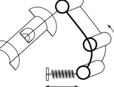
Newtonian mechanics are well and good, when one deals with one or several point-like objects moving freely in space, such as the Sun and the planets (even though these problems are in no way trivial). Now suppose you have a complex mechanism like one of those contraptions the Victorians were so adept

at building (Figure 1.10) and need to predict its behaviour. Describing everything in terms of positions of different parts of the mechanism in real space would be incredibly messy and impractical. For example, why give the positions and velocities in the real space of the ends of a rigid lever in 12 numbers, which can be completely described by just two numbers – a rotation angle and the corresponding angular velocity? But on the other hand, we do need positions, velocities and accelerations in the real space in order to write down the second law!

Figure 1.10 a mechanical contraption, which is hard to describe by

cartesian coordinates

This difficulty became clear before Hamilton’s time, and was eventually resolved by another great scientist, Lagrange. He developed a very useful and insightful approach – Lagrangian mechanics – that served as the basis for the Hamiltonian one, which is very much in use and also very important for the modern quantum physics. We will discuss this further in Chapter 9.

Spotlight: Lagrange equations

Lagrange equations – just to impress you. We will only need them in Chapter 9. d dt L q q q L q q q ( , ) ( , ) 0.    ∂ ∂    − ∂ ∂ =

The gist of it is that Lagrange developed a method of describing an arbitrary mechanical system by a set of generalized

coordinates, q_i and generalized velocities, q˙_i≡ dq˙i /dt. These

coordinates can be any convenient parameters that describe our mechanical system: rotation angles; elongations; distances; or even conventional positions in real space. The index i _{= 1, 2, …, M labels these coordinates; M is the number of} the degrees of freedom our system possesses. Please note that, by tradition and for brevity, for the generalized velocities the Newtonian notation for a time derivative is used.

Key idea: Phase and configuration spaces

..., x_N,p_xN,y_N,p_yN,z_N,p_zN) which completely describe a set of N particles in three-dimensional space, can be thought of as coordinates of a single particle in a 6N-dimensional phase space of the system. If we are only interested in the positions of these particles, we can also describe the system as a single point with coordinates (x₁,y₁,z₁, ..., x_N,y_N,z_N), which moves in a 3N-dimensional configuration space. In either case, our investigation of a totally mundane system of classical particles in a conventional three-dimensional space takes us to pretty esoteric spaces.

Lagrange discovered how to write a certain function – the Lagrangian, L(q, q˙) – of all these variables, which satisfies certain differential equations, from which all the generalized coordinates q_i(t) can be found for all later moments of time, provided that we specify the initial conditions: q_i(0) = q0i;

q˙_i(0) = q˙0i. Moreover, he proved that these equations are

equi-valent to those following directly from Newton’s second law, even though the former are much easier to write down than the latter. As before, we can take the set of all generalized coordinates and consider them as the coordinates of a single point in an M-dimensional configuration space. And, as before, we can introduce the phase space (which will be, of course, 2M-dimensional), the state vector in this space, and the

Hamilton’s equations. That is, Hamilton did it. In particular, he discovered how – starting from a Lagrangian – one can find the momentum p_i , corresponding to a given generalized coordinate q_i. It is called the canonical momentum and is often something very unlike m_iq˙_i . Then he showed how to obtain from the Lagrangian L(q,q˙) the Hamiltonian H(q,p). And then one can immediately write down and – with some luck and much hard work – solve the Hamilton’s equations and find the behaviour of the system:

=∂ ∂ dq dt H p ; i i = −∂ ∂ dp dt H q ; i i i _{= 1,2, ... 2M}

In many cases these equations are easier to solve than the Lagrange equations. What is more important to us is that they form a vital link between quantum and classical mechanics. Hamilton’s equations describe the evolution with time of the state vector in a 2M-dimensional phase space of our system. One cannot easily imagine this, but some geometrical intuition based on our lower-dimensional experience can be actually developed with practice. For example, you can draw the phase trajectories in each of the M planes (q_i ,p_i) and consider them in the same way one does different projections of a complex piece of machinery in a technical drawing.

We will try to show how it works on another example – the last in this chapter – of those notions from classical physics, which turn out to be not that much different from their quantum counterparts.

Statistical mechanics, statistical

ensemble and probability

distribution function

One of the simplest and most useful model systems considered by classical physics is the monoatomic ideal gas – a collection of a very large number N of identical material points, which do not interact with each other. This model helped establish the fundamentals of statistical mechanics – the aspect of physics that explains, in particular, why water freezes and how an electric heater works. We already know that the state of this system can be completely described by a state vector in a 6N-dimensional phase space (or, which is the same, a single point in this space – the end of the state vector; see Figure 1.9).

As we know, the state vector determines all the positions (in real space) and all the momenta of all N gas particles. A single cubic centimetre of gas at normal pressure and zero degrees Celsius contains about 2.7 × 1019 _{molecules. Therefore}

the state vector contains a lot of unnecessary and unusable information. It is unusable, because even if we had all this information, we could never solve 6 × 2.7 × 1019 _Hamilton’s

equations per cubic centimetre of gas. Unnecessary, because we do not care where precisely each gas particle is placed and what momentum it has at a given moment of time. We are interested in bulk properties, like temperature, pressure, local flow velocity and so on at a given position in a given moment of time.

The central point of statistical mechanics makes it so that a single set of such bulk properties (P(r, t), T(r, t), v(r, t), ...) – a so-called macroscopic state of our system – corresponds to a huge number of slightly different microscopic states (each described by a state vector in the 6N-dimensional phase space). These are found in the vicinity of certain point R _{= (q, p) in this} space (Figure 1.11), which has ‘volume’ ∆Г(q, p).

p3 p2 Δr p1 q4 q3 q2 q1 p3N q3N R … …

Figure 1.11 a statistical ensemble in phase space

Spotlight: Distribution functions and

statistical ensembles

The distribution functions and equation for f₁ (the Boltzmann equation) were introduced by Ludwig Boltzmann (1844–1906). The concept of statistical ensembles was proposed by Josiah Willard Gibbs (1839–1903).

One way to use this idea is to introduce a statistical ensemble of N-particle systems – that is, a very large number N_E of copies of our system with slightly different initial conditions. They will form something like a ‘cloud of gas’ in the phase space, and each will follow its own unique trajectory determined by the Hamilton’s equations. (The fact that in practice we cannot solve or even write down these equations does not matter in the least!) To calculate the likelihood of finding our system in a given macroscopic state, we can simply count how many of N_E systems in the ensemble are found in the ‘volume’ ΔГ(q, p) at a given moment. Now denote this number ΔN_E(q, p, t) and introduce the function

q p = _{→ ∞} ∆ q p f t _N N t N ( , , ) lim ( , , ). N E E E

This function is called the N-particle probability distribution (or simply distribution) function. It gives the probability to find the system in a given microscopic state (because it still depends on all the momenta and all the positions of all the particles). Obviously, this is not much of an improvement, since this is as detailed a description, as we had initially, and the equations of motion for this function are as many, as complex and as unsolvable as the Hamilton’s equations for all N particles. But once we have introduced the distribution function, some drastic simplifications become possible. To begin with we can ask what the probability is for one gas particle to have a given position and momentum at a given time. Let us denote it as

f₁(q, p, t),

where now (q, p) are the position and momentum of a single particle in a phase space with a miserly six dimensions. Since all gas particles are the same, the answer will do for any and for all of them. Moreover, properties such as temperature or pressure, which determine the macroscopic state of gas, can be calculated using only f₁(q, p, t). Finally, the approximate equations, which determine the behaviour of f₁(q, p, t), can be written down and solved easily enough.

Sometimes we would need to know the probability that one particle has the position and momentum (q₁, p₁), and other (q₂, p₂), simultaneously. The approximate equations for the corresponding two-particle distribution function, f₂(q, p, t), can be also readily written down and – with somewhat more trouble – solved. Such equations can be written for all distribution functions, up to the N-particle one from which we started, but in practice physicists very rarely need any distribution functions beyond f₁(q, p, t) and f₂(q, p, t). The idea that sometimes we can and need to know something only on average is a very powerful idea.4 _{It allowed the great}

progress of classical statistical mechanics. We will see how it is being used in quantum mechanics.

4 In statistical mechanics, knowledge is power, but ignorance (of unnecessary data) is might!

Liouville equation*

One last remark: the N-particle distribution function f_N(q, p, t) changes with time, because the coordinates and momenta also change with time. One can derive the equation for f_N(q, p, t):

q p

_∑

which is essentially the result of applying the chain rule of differentiation to the time derivative of f_N(q, p, t). This equation describes the ‘flow’ in the phase space of the points, which represent the individual systems in the statistical ensemble. Since the total number of systems in the ensemble is constant, the full time derivative of f_N(q, p, t) must be zero. For the partial time derivative, which describes how f_N(q, p, t) changes in time at a fixed point (q, p) in the phase space, we therefore obtain the Liouville equation, q p

∑

Fact-check

?

3 In order to predict the behaviour of a material point you need to know its initial

a position

b position and velocity c velocity and acceleration d position and momentum

4 How many dimensions does the phase space of a system with nine spring pendulums have?

a 3 b 9 c 54 d 18

5 How many dimensions does the configuration space of the same system have?

a 3 b 9 c 54 d 18

6 The phase trajectory of a harmonic oscillator can have the following shape:

a parabola b hyperbola c ellipse d circle

7 Indicate impossible trajectories of a material point in real space

(d) (c) (a) (b) x px

8 Indicate possible trajectories of a material point in the phase space _(d) (c) (a) (b) x px

9 Conjugate variables are a x and p_y

b p_x and p_z c z and p_z d x and y

10 Hamilton’s equations directly describe the evolution of a mechanical system in real space

b state vector in phase space c state vector in configuration space d only of a harmonic oscillator

Dig deeper

Further reading I. Some serious reading on classical mechanics and related mathematics.

R. Feynman, R. Leighton and m. sands, Feynman Lectures on Physics, Vols i, ii and iii. Basic Books, 2010 (there are earlier editions). see in particular Vol. i (read there about mechanics and some mathematics, chapters 1–25).

P. hamill, A Student's Guide to Lagrangians and Hamiltonians. cambridge university Press, 2013.

F. Reif, Statistical Physics, Berkeley Physics course, Vol. 5. mcGraw-hill Book company, 1967.

L. susskind and G. hrabovsky, Theoretical Minimum: What You Need to Know to Start Doing Physics. Basic Books, 2013. here is a really welcome book: classical mechanics, including its more arcane sides (like phase space and hamilton equations), presented in an accessible form! susskind is a prominent string theorist, which makes it even more interesting.

Ya. B. Zeldovich and i. m. Yaglom, Higher Math for Beginning Physicists and Engineers. Prentice hall, 1988. introduces mathematical tools together with the physical problems they were developed to solve, and teaches learners how to use these tools in practice.

Further reading II. About the ideas and scientists.

V.i. arnold, Huygens & Barrow, Newton & Hooke. Birkhauser, 1990. the same story, told by a great mathematician from his unique point of view, and much more.

J. Bardi, The Calculus Wars. high stakes Publishing, 2007. how newton and Leibniz discovered calculus.

L. Jardine, The Curious Life of Robert Hooke: The Man who Measured London. harper Perennial, 2004. a very good biography. t. Levenson, Newton and the Counterfeiter. Faber & Faber, 2010. a fascinating story of how newton managed the Royal mint, tracked and caught a gang of counterfeiters, and had their chief executed.

2

Less familiar

physics in stranger

spaces

The objective of the previous chapter was to glance at classical mechanics from a less familiar angle.

Now we will try and look at quantum mechanics from this angle, in the hope that it will look somewhat less strange – or at least no stranger than it must. This is not how it was seen by its founders, but it is only natural: highways rarely follow the trails of the first explorers.

Let us start from the beginning. In 1900, Professor Max Planck of the University of Berlin introduced the now famous Planck constant h _{= 6.626…·10}–34 _{J s. For very compelling reasons,}

which we will not outline here, Max Planck made the following drastic prediction concerning harmonic oscillators, which in modern terms went as follows:

A harmonic oscillator with frequency ν0 can change its energy

only by an amount hν0 (the so-called energy quantum, from the

Latin quantus meaning ‘how much’). In other words, ∆E = hνo.

Initially Planck referred to what we now call ‘energy quantum’ of an oscillator as one of ‘finite equal parts’ of vibrational energy. The term ‘quantum’ was coined later. One of its first users, along with Planck, was Philipp Lenard, a first-rate experimentalist, whose work greatly contributed to the discovery of quantum mechanics, and who was also – regrettably – a first-rate example of how a brilliant physicist can go terribly wrong outside his field of expertise. But, no matter what terms were used, the notion of deriving discrete portions of energy from an oscillator was revolutionary.

Key idea: Planck constant

In modern physics literature, the original Planck constant h _{= 6.2606957(29)•10}–34 _{J s is used less frequently than ħ} (pronounced ‘eichbar’): h 2 1.054571726(47) 10 J s. 34  π = = ⋅ −

Both are usually called ‘the Planck constant’.

The figures in brackets indicate the accuracy to which this constant is currently known. Roughly speaking, if some A = 1.23(45), it means that A is most likely equal to 1.23, but can be as small as 1.23 – 0.45 = 0.78 or as large as 1.23 + 0.45 = 1.68.