HAL Id: tel-02926078
https://tel.archives-ouvertes.fr/tel-02926078
Submitted on 31 Aug 2020
HAL is a multi-disciplinary open access
archive for the deposit and dissemination of sci-entific research documents, whether they are pub-lished or not. The documents may come from teaching and research institutions in France or
L’archive ouverte pluridisciplinaire HAL, est destinée au dépôt et à la diffusion de documents scientifiques de niveau recherche, publiés ou non, émanant des établissements d’enseignement et de recherche français ou étrangers, des laboratoires
Suspended sediment production and transfer in
mesoscale catchments : a new approach combining flux
monitoring, fingerprinting and distributed numerical
modeling
Magdalena Uber
To cite this version:
Magdalena Uber. Suspended sediment production and transfer in mesoscale catchments : a new approach combining flux monitoring, fingerprinting and distributed numerical modeling. Applied geology. Université Grenoble Alpes [2020-..], 2020. English. �NNT : 2020GRALU011�. �tel-02926078�
TH `
ESE
Pour obtenir le grade de
DOCTEUR DE L’UNIVERSIT ´
E GRENOBLE ALPES
Sp ´ecialit ´e : Oc ´ean, Atmosph `ere, Hydrologie
Arr ˆet ´e minist ´eriel : 25 Mai 2016 Pr ´esent ´ee par
Magdalena Uber
Th `ese dirig ´ee parC ´edric Legout
et coencadr ´ee parGuillaume Nord
pr ´epar ´ee au sein d’Institut des G ´eosciences de l’Environnemenet (IGE)
dans l’ ´Ecole DoctoraleTerre Univers Environnement
Suspended sediment production and
transfer in mesoscale catchments: a new
approach combining flux monitoring,
fingerprinting and distributed numerical
modeling
Th `ese soutenue le9 juin 2020,
devant le jury compos ´e de :
Fr ´ed ´eric Li ´ebault
Directeur de Recherche, INRAE Grenoble, Pr ´esident
N ´uria Mart´ınez-Carreras
Researcher, Luxembourg Institute of Science and Technology, Rapporteur
Axel Bronstert
Professeur, University of Potsdam, Rapporteur
Agn `es Ducharne
Directrice de Recherche, METIS, Sorbonne Universit ´e, Examinatrice
Anne Probst
Directrice de Recherche, ECOLAB, Examinatrice
Luis Cea
Senior lecturer, Universidade da Coru ˜na, Examinateur
Acknowledgements
I would like to thank many people at IGE or elsewhere, without them this work would not have been possible or less pleasant:
First and foremost a big thank you to C´edric and Guillaume for the ex-cellent supervision, for having initiated this PhD project, for your support, creativity, encouragement and understanding throughout the last three-and-a-half years. This thesis is a result of team work and it was always a pleasure to work with you!
I also want to thank those who contributed to this thesis in one way or another: J´erˆome Poulenard, Christian Crouzet, Fran¸cois Demory, Nico Hachgenei, Brice Boudevillain, Olivier Evrard, Ir`ene Lef`evre and especially Luis Cea. Thank you, Luis, for welcoming me in A Coru˜na, for your ongoing support in the modeling studies and for your fast help whenever I encoun-tered a problem.
Further, I would like to thank Luis, Brice, J´erˆome and Isabelle Braud for the very fruitful and always constructive discussions during the meetings of my Comit´e de th`ese. I also thank the reviewers of this thesis, N´uria Mart´ınez-Carreras and Axel Bronstert for their detailed lecture of the manuscript, their very constructive comments and their interest and acknowledgement of this work as well as the other members of the Jury Fr´ed´eric Li´ebault, Anne Probst, Agn`es Ducharne and Luis Cea for the very pleasant and fruitful discussion during the PhD defense. Thanks to all the researchers, students and tech-nicians involved in the OHMCV and Draix-Bl´eone observatories for having generated such valuable data sets and for the inspiring meetings in Grenoble and Draix.
I also want to thank IGE’s administrative service, especially Carm´eline, Odette and Val´erie, Christine and Florence from the doctoral school for your constant help with administrative issues as well as to Mondher for the help with the calculations. Most of the calculations presented here were performed using the GRICAD infrastructure whose staff I want to thank for this service. A big thank you also to my friends in the lab, the fellow PhD students and interns for all the time we spent together and for being there for each other: Catherine, Claudio, Maria Belen, Ana, Stefano, Mathilde and Alessandra; Pati and Gabriela, you were wonderful office mates, thank you for the nearly three years we spent in office 108. Thank you also to Nico, An and Romane for your company and the nice moments during those last stressful months of writing and to the many other PhD students and colleagues who made IGE a very pleasant working environment.
Thank you to my friends outside the lab for having made the time in Grenoble such a wonderful experience: to Johannes for the nice hikes in the mountains; to Nico and many others at Les pouces verts for sharing more than fruits and vegetables; to Meike, Jan, Arthur, Melli, Fabien, Agnieszka, Cecilia, Andrea, Pauline and Alban for sharing the parenting experience; to Oc´e, Laura, Nadia, Diego, Nino, Abdul, Arturo and Thomas for your con-viviality and friendship.
To all my friends in Berlin, especially to Lea, Johan and Paula for always welcoming us in your flat and for making me feel as if I never left when I was back in my home town. You are the best!
I also owe a big thank you to the regular and occasional babysitters, without you I would still be writing the introduction! Especially to Bernd, who always came running from various parts of Europe to take care of a sick granddaughter when we needed help and to Gertrud, Helmut and Silja for your invaluable aid during the last months in home office and Corona confinement.
Last but not least a big thank you to Linus for all your support and companionship during all those years and to Flora for being the best kid ever. You are the best family I could imagine and I am looking forward to new adventures with you!
R´
esum´
e
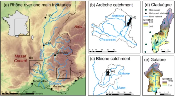
L’´etude des m´ecanismes d’´erosion hydrique des sols et de transfert de mati`eres en suspension (MES) des bassins versants vers les rivi`eres revˆet des enjeux environnementaux et socio-´economiques pr´egnants face `a une pression an-thropique grandissante et au changement climatique. L’objectif de cette th`ese est de comprendre comment la variabilit´e de la pluie contrˆole l’activation de diff´erentes zones sources de MES et la dynamique des flux hydro-s´edimentaires dans deux bassins versants m´editerran´eens de m´eso-´echelle, la Cladu`egne (42 km2) et le Galabre (20 km2) membres de l’infrastructure de recherche sur la zone critique OZCAR.
Dans la premi`ere partie, les contributions des zones d’´erosion aux MES `a l’exutoire de la Cladu`egne ont ´et´e quantifi´ees `a haute r´esolution temporelle avec une approche low-cost de tra¸cage. Deux ensembles de traceurs (spec-tres colorim´etriques et de fluorescence X) et trois mod`eles de m´elange ont ´et´e compar´es pour ´evaluer la sensibilit´e des contributions de sources `a ces choix m´ethodologiques. Les principales sources de MES identifi´ees sont les zones de badlands marno-calcaires. Une approche similaire conduite sur le bassin ver-sant du Galabre a mis en avant la dominance des badlands sur molasses dans les flux de MES. La comparaison des traceurs et des mod`eles de m´elange, a montr´e que les choix m´ethodologiques g´en`erent des diff´erences importantes, qui am`enent `a recommander une approche d’ensemble multi-traceurs-multi-mod`ele pour obtenir des r´esultats plus robustes. L’application de cette ap-proche `a un grand nombre d’´echantillons de MES a soulign´e l’importante variabilit´e inter et intra ´ev`enements des contributions des diff´erentes sources de MES, soulevant des questions sur les processus hydro-s´edimentaires `a l’origine de la variabilit´e des flux de MES.
l’hypo-th`ese que cette variabilit´e r´esultait de distributions des temps de transfert des MES tr`es variables contrˆol´ees par i) les caract´eristiques inh´erentes aux bassins versants comme la localisation des diff´erentes sources de MES et la fa¸con dont elles sont li´ees `a l’exutoire (i.e. connectivit´e structurelle) et ii) les caract´eristiques spatio-temporelles des ´ev`enements pluvieux qui activent et impactent les vitesses de transfert (i.e. connectivit´e fonctionnelle). Ainsi, dans la deuxi`eme partie, un mod`ele num´erique distribu´e bas´e sur la r´esolution des ´equations de Saint Venant coupl´e `a un module d’´erosion multi-sources de MES, a ´et´e utilis´e pour ´evaluer les rˆoles respectifs des connectivit´es struc-turelle et fonctionnelle. L’analyse de sensibilit´e aux choix de discr´etisation et de param´etrisation (i.e. seuil d’aire drain´ee pour distinguer la rivi`ere des versants, valeurs de coefficients de frottement sur les versants et la rivi`ere) a montr´e que la localisation des sources de MES dans le bassin versant ´etait plus importante que les choix de mod´elisation `a condition que les param`etres soient dans une gamme r´ealiste et limit´ee. Un sch´ema g´en´eral de r´eponse tem-porelle du bassin versant par type de sources a ´et´e observ´e, coh´erent avec les r´esultats de l’approche de tra¸cage et la distribution des distances des sources `
a la rivi`ere et `a l’exutoire. Ce mˆeme sch´ema persiste pour diff´erentes dur´ees ou intensit´es des pr´ecipitations mais devient beaucoup plus variable lorsque des hy´etogrammes bimodaux ou des pr´ecipitations variables dans l’espace sont appliqu´ees. En outre, la localisation de la pluie par rapport aux sources d´etermine les contributions moyennes des sources et donc les diff´erences entre les ´ev´enements de pluie.
Les deux approches de tra¸cage des MES et de mod´elisation num´erique se sont av´er´ees compl´ementaires et leur application combin´ee pr´esente un fort potentiel pour comprendre comment les interactions entre connectivit´e structurelle et fonctionnelle contrˆolent la dynamique des flux de MES aux exutoires de bassins versants de m´eso-´echelle.
Abstract
The study of soil erosion by water and the transfer of suspended solids from watersheds to rivers is crucial given the environmental and socio-economic is-sues with regards to growing human influence and the expected intensification of these processes under climate change. The objective of this thesis is to un-derstand how rainfall variability controls the activation of different sediment source zones and the dynamics of hydro-sedimentary flows in two mesoscale Mediterranean catchments, i.e. the Cladu`egne (42 km2, subcatchment of the Ard`eche) and the Galabre (20 km2, subcatchment of the Durance) which are members of the OZCAR critical zone research infrastructure.
In the first part, the contributions of the erosion zones to sediment fluxes at the outlet of the Cladu`egne catchment were quantified at high tempo-ral resolution with a low-cost sediment fingerprinting approach. Two sets of tracers (color and X-ray fluorescence tracers) and three mixing models were compared to assess the sensitivity of estimated source contributions to these methodological choices. Marly-calcareous badlands were identified as the main sediment source. A similar approach carried out on the Galabre catchment area showed that badlands on molasses were the main source. The comparison of tracer sets and mixing models, showed that the methodologi-cal choices generated important differences. Thus, we suggest a multi-tracer-multi-model ensemble approach to obtain more robust results. The appli-cation of this approach to a large number of sediment samples highlighted the important within and between event variability in the contributions of different sediment sources, raising questions about the hydro-sedimentary processes that cause this variability.
We hypothesized that this variability resulted from variable suspended sediment transit time distributions governed by the interplay of (i)
catch-ment characteristics such as the location of different sources and how they are linked to the outlet (referred to as structural sediment connectivity) and (ii) the spatio-temporal characteristics of rain events that activate and im-pact transfer velocities (i.e. functional connectivity).
Thus, in the second part, a distributed numerical model based on the resolution of the Saint Venant equations coupled to a multi-source erosion module was used to evaluate the respective roles of structural and functional connectivity. Sensitivity analysis of the discretization and parameterization choices (i.e. threshold of contributing drainage area to identify the river network, values of roughness coefficients on hillslopes and the river) showed that the location of the sediment sources in the watershed was more impor-tant than the modeling choices when the parameters were limited to realistic range. A general temporal pattern of source contributions was observed. This was consistent with the results of the fingerprinting approach and the distribution of distances from the sources to the river and the outlet. The same pattern persists for different rainfall durations or intensities but became much more variable when bimodal hyetographs or spatially variable precip-itation was applied. In addition, the location of the rainfall with respect to the sources determined the average contributions of the sources and thus differences between rainfall events.
The two approaches, sediment fingerprinting and numerical modeling, were found to complement each other. Their combined application has a high potential for understanding how interactions between structural and functional connectivity control the dynamics of sediment fluxes in mesoscale catchments.
Contents
Acknowledgements 2 R´esum´e 4 Abstract 6 List of Figures 14 List of Tables 15 1 Introduction 16 1.1 Motivation . . . 16 1.2 Scientific context . . . 201.2.1 Soil erosion and sediment transport . . . 20
1.2.2 Sediment connectivity . . . 24
1.2.3 Sediment fingerprinting . . . 29
1.2.4 Modeling soil erosion and sediment transport . . . 33
1.3 Objectives . . . 42
2 Study sites 45 2.1 Cladu`egne catchment. . . 46
2.1.1 Introduction . . . 46
2.1.2 Geology, soils and topography. . . 46
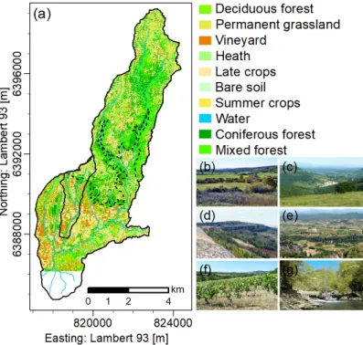
2.1.3 Land cover . . . 48
2.1.4 Erosion zones . . . 49
2.1.5 Climate . . . 50
2.1.6 Hydrology . . . 51
2.1.7 Soil erosion and sediment export . . . 55
2.1.8 Data availability . . . 56
2.2.1 Introduction . . . 59
2.2.2 Geology, soils and topography. . . 60
2.2.3 Land cover and erosion zones . . . 61
2.2.4 Climate . . . 62
2.2.5 Hydrology . . . 63
2.2.6 Soil erosion and sediment export . . . 66
2.2.7 Data availability . . . 67
3 High temporal resolution quantification of suspended sediment source contributions in two mesoscale Mediterranean catchments 70 3.1 Cladu`egne . . . 70
3.1.1 Introduction . . . 72
3.1.2 Methods . . . 73
3.1.2.1 Sampling . . . 73
3.1.2.2 Measurements of tracer properties . . . 74
3.1.2.3 Tests of assumptions. . . 76
3.1.2.4 Source quantification with mixing models . . . 77
3.1.2.5 Error assessment . . . 79
3.1.3 Results . . . 82
3.1.3.1 Verification of fingerprinting assumptions . . . 82
3.1.3.2 Comparison of the mixing models . . . 83
3.1.3.3 Comparison of the tracer sets. . . 85
3.1.3.4 Errors of the fingerprinting approaches . . . 89
3.1.4 Discussion. . . 92
3.1.4.1 Performance and errors of the various fingerprint-ing approaches . . . 92
3.1.4.2 Interests of using multi-tracer-model ensemble pre-dictions to detect main sources, within- and be-tween event variability in a mesoscale catchment . 94 3.1.5 Conclusions and perspectives . . . 100
3.2 Galabre . . . 102
3.2.1 Introduction . . . 102
3.2.2 Materials and methods. . . 102
3.2.3 Results and discussion of the previous studies . . . 103
3.2.4 Conclusions and perspectives . . . 106
3.3 Temporal variability of suspended sediment fluxes . . . 107
3.3.1 Variability between flood events . . . 107
3.3.2 Variability within flood events . . . 108
4 Variability in source soil contributions to suspended sediments:
the role of modeling choices and structural connectivity 115
4.1 Introduction. . . 115
4.2 Methods . . . 117
4.2.1 Characteristics of the modeled study sites . . . 117
4.2.2 Model description . . . 120
4.2.3 Model discretization and input data . . . 122
4.2.4 Modeling scenarios . . . 124
4.2.5 Comparison of scenarios . . . 127
4.3 Results and discussion . . . 128
4.3.1 Impact of modeling choices on modeled sediment dynamics 128 4.3.1.1 Varying the contributing drainage area threshold . 128 4.3.1.2 Varying Manning’s n . . . 133
4.3.2 The role of structural connectivity on the dynamics of sus-pended sediment fluxes at the outlet . . . 136
4.4 Conclusions and perspectives . . . 141
5 Variability in source soil contributions to suspended sediments: the role of spatio-temporal rainfall variability 143 5.1 Introduction. . . 143
5.2 Precipitation data quality control . . . 147
5.3 Methods . . . 153
5.3.1 Selected rain events . . . 153
5.3.1.1 Cladu`egne . . . 153
5.3.1.2 Galabre . . . 155
5.3.2 Rainfall forcing used in the modeling scenarios . . . 158
5.3.2.1 Temporal rain variability . . . 158
5.3.2.2 Spatial rain variability. . . 159
5.3.2.3 Location of the storm . . . 161
5.4 Results and discussion . . . 162
5.4.1 How does temporal variability of rainfall forcing impact sim-ulated hydro-sedimentary fluxes of different sediment sources?162 5.4.2 Does spatial variability of rainfall forcing impact modeled hydro-sedimentary fluxes in mesoscale catchments? . . . 169
5.4.2.1 Impact of simplifications of rainfall patterns . . . 169
5.4.2.2 Impact of neglecting spatial rainfall variability . . 174
5.4.3 How does the location of rain cells with respect to the sources determine source contributions to sediment fluxes at the out-let? . . . 177
6 Conclusions and perspectives 182
6.1 Comparison of model results with source contributions estimated
with sediment fingerprinting . . . 182
6.2 Synthesis and future research directions . . . 188
6.2.1 Where do suspended sediments passing the outlet of two
mesoscale catchments originate and how do the
contribu-tions of different sources vary within and between flood events?188
6.2.2 What are the reasons for the observed variability of source
contributions between and within events? . . . 190
6.2.3 Benefits of combining sediment fingerprinting and distributed
numerical modeling . . . 195
Appendices 197
A Calculation of specific sediment yield 198
B Supplementary information for Chapter 3.1 200
B.1 Additional figures and tables . . . 200
B.2 Comparison of the alternative tracer sets with conventional
finger-printing . . . 203
C Supplementary information for Chapter 4 206
C.1 Additional figures and tables . . . 206
D Supplementary information for Chapter 5 210
D.1 Precipitation data criticism (Chapter 5.2) . . . 210
D.2 Additional figures. . . 213
List of Figures
1.1 Sediment yield in Europe (Vanmaercke et al., 2011). . . 18
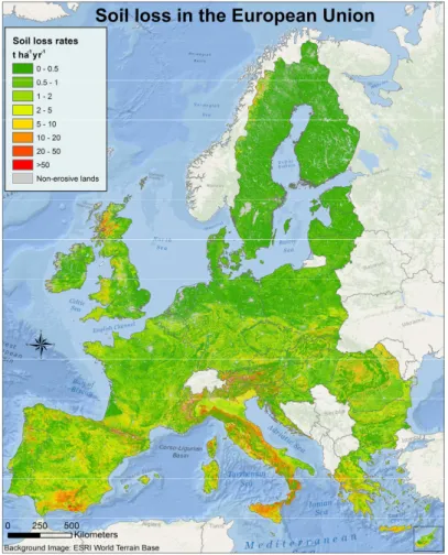
1.2 Map of soil loss in Europe (Panagos et al., 2015b) . . . 19
1.3 Types of soil erosion by water . . . 21
1.4 Sediment transport in rivers . . . 23
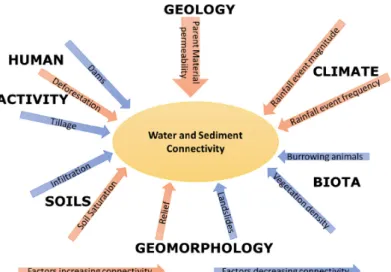
1.5 Factors controlling water and sediment connectivity (Keesstra et al., 2018). . . 25
1.6 Conceptual framework of connectivity by Fryirs (2013). . . 27
1.7 Scheme of sediment fingerprinting. . . 30
1.8 Variability in SSC − Ql relation . . . 36
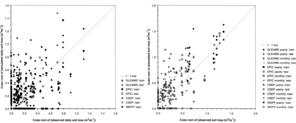
1.9 Observed and simulated soil loss (Jetten et al., 1999) . . . 37
1.10 Observed and simulated soil loss (Alewell et al., 2019) . . . 38
1.11 Combining fingerprinting and erosion modeling (Palaz´on et al., 2016) 41 2.1 Location of the study sites . . . 45
2.2 Geology and pedology of the Cladu`egne catchment . . . 47
2.3 Land cover of the Cladu`egne catchment . . . 48
2.4 Erosion zones in the Cladu`egne catchment . . . 49
2.5 Cladu`egne river during low flow and during a flash flood . . . 52
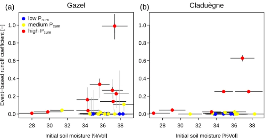
2.6 Initial soil moisture and event based runoff coefficients . . . 53
2.7 Annual hydro-sedimentary dynamics (Cladu`egne) . . . 54
2.8 Geology of the Galabre catchment . . . 60
2.9 Land cover of the Galabre catchment . . . 61
2.10 Monthly precipitaion at Laval (Mathys, 2006) . . . 63
2.11 Intra-annual hydro-sedimentary dynamics (Galabre) . . . 64
2.12 Galabre river during low flow and during a flash flood . . . 65
3.1 Sampling sites for sediment fingerprinting (Cladu`egne). . . 74
3.2 Comparison of different mixing models in sediment fingerprinting . 84 3.3 Comparison of different tracer sets in sediment fingerprinting . . . 86
3.4 Source contributions during a flood event in 2013 . . . 87
3.6 Comparison of spectral tracers with radionuclids . . . 89
3.7 Mean source contributions in the Cladu`egne and Gazel . . . 95
3.8 Mean source contributions in the Gazel catchment . . . 97
3.9 Between event variability of sediment source contributions . . . 98
3.10 Within event variability of source contributions . . . 99
3.11 Sampling sites for sediment fingerprinting (Galabre) . . . 103
3.12 Discrimination of sources with color and DRIFTS tracers . . . 104
3.13 Comparison of results obtained with color and DRIFTS tracers . . 105
3.14 Between event variability of source contributions (Cladu`egne).. . . 107
3.15 Between event variability of source contributions (Galabre). . . 108
3.16 Scheme of classification of events due to sediment flux variability . 109 3.17 Within event variability of source contributions . . . 110
3.18 Source contributions during different stages of the hydrograph. . . 111
3.19 Distributed event Precipitation for two events . . . 114
4.1 Distance of the sources to the outlet and the stream . . . 118
4.2 Characteristic times of hydrographs and sedigraphs . . . 127
4.3 Simulated hydrographs with different CDA thresholds . . . 129
4.4 Sensitivity to characteristic times to changing model parameters . 130 4.5 Simulated sedigraphs with different CDA thresholds . . . 131
4.6 Modeled source contributions with varying CDA thresholds . . . . 132
4.7 Modeled hydrographs and sedigraphs with varying Manning’s n . . 133
4.8 Modeled source contributions nhillsl. = 0.2 . . . 134
4.9 Hydro-sedimentary fluxes: distance to the outlet (Galabre) . . . . 138
4.10 Hydro-sedimentary fluxes: distance to the stream (Galabre) . . . . 139
5.1 Comparison of radar and rain gauge data (Galabre) . . . 150
5.2 Difference of rainfall in the north and south of the catchments. . . 152
5.3 Rain events in the Cladu`egne catchment . . . 154
5.4 Rain events in the Galabre catchment . . . 156
5.5 Scheme of rainfall forcing: temporal variability . . . 158
5.6 Scheme of rainfall forcing: spatial variability. . . 160
5.7 Locations of artificial storms passing the catchments . . . 164
5.8 Modeled source contributions with varying rain intensity and duration165 5.9 Modeled hydro-sedimentary fluxes obtained with bimodal hyetographs166 5.10 Hydro-sedimentary fluxes modeled with real and approximated hyeto-graphs . . . 168
5.11 Comparison of distributed radar data and elliptic approximation . 171 5.12 Comparison of distributed radar data and approximated precipi-taion gradient . . . 172
5.13 Comparison of distributed and uniform precipitation . . . 175
5.14 Role of the location of the storm . . . 178
6.1 General pattern of modeled source contribution . . . 184
6.2 Modeled source contributions during different stages of the hydrograph186
A.1 SSC - T relation in the two catchment . . . 199
B.1 Effect of particle size on tracer values . . . 202
B.2 Predicted vs. real source contributions to artificial mixtures . . . . 202
B.3 Source contributions predicted with radionuclids . . . 205
C.1 Structural connectivity of potential sediment sources . . . 207
C.2 Hydro-sedimentary fluxes: distance to the outlet (Cladu`egne) . . . 209
C.3 Hydro-sedimentary fluxes: distance to the stream (Cladu`egne) . . 209
D.1 Cumulated radar precipitation data . . . 211
D.2 Criticism of rain gauge data (Galabre) . . . 212
D.3 Residuals of radar and rain gauge data (Cladu`egne) . . . 213
D.4 Seasonality of agreement of radar and rain gauge data (Cladu`egne) 214
D.5 Seasonality of agreement of radar and rain gauge data (Galabre) . 215
List of Tables
2.1 Specific yield of Mediterranean catchments . . . 56
3.1 Sampling for sediment fingerprinting and tests of assumptions . . . 75
3.2 Estimates of error of the 3 mixing models and 2 tracer sets . . . . 90
4.1 Characteristics of the catchments and the erosion zones . . . 119
4.2 Modeling scenarios . . . 125
4.3 Scheme of responses of Ql and Qs to changes in Manning’s n . . . 134
5.1 Scores of agreement of radar and rain gauge data . . . 149
5.2 Modeling scenarios: temporal rain variability . . . 159
5.3 Modeling scenarios: spatial rain variability and storm location . . 162
5.4 Characteristics of modeled hydrographs and sedigraphs: temporal variability . . . 163
5.5 ∆t,crit for independent events . . . 167
5.6 Characteristics of modeled hydrographs and sedigraphs: spatial variability . . . 170
6.1 Group classification in Fingerprinting and modeling . . . 183
B.1 Selected tracer statistics . . . 201
B.2 Selected radionuclid tracers . . . 203
B.3 Error due to source heterogeneity (radionuclid tracers) . . . 204
Chapter 1
Introduction
1.1
Motivation
Soil erosion and sediment transport are important processes that shape the critical zone, i.e. “the thin layer of the Earth’s terrestrial surface and near-surface environment that ranges from the top of the vegetation canopy to the bottom of the weathering zone” (Guo and Lin, 2016). These natural processes create diverse ecosystems such as braided river systems and river deltas that are a habitat to many species. However, as human activities in the Anthropocene are exerting profound influence on all compartments of the environment (Crutzen,2006; Zalasiewicz et al.,2008), there is an increasing anthropogenic impact on these processes (Syvitski and Kettner, 2011; Poe-sen,2018). Via land cover changes and climate change, erosion is accelerated in a way that it now exceeds rates of soil production by many in large parts of the world (Montgomery,2007). On the other hand, sediments are retained in reservoirs behind dams and do not reach the ocean, leading to a disturbance of natural balances in floodplains and deltas (Syvitski and Kettner, 2011).
Excess erosion and sediment export from headwater catchments to river systems and the ocean can cause important on-site and off-site problems. The former concerns mainly soil loss and the associated loss of nutrients and fertile topsoil and thus a decrease of agricultural productivity (Pimentel
et al., 1995; Amundson et al., 2015; Panagos et al., 2015b). Soil erosion
by water is considered one of the main threats to soils in Europe (Panagos
the sediment balance of downstream water bodies which cause the loss of reservoirs capacities due to siltation and thus necessitate regular and costly dredging activities or flushing (Camenen et al., 2013; Wisser et al., 2013;
Kondolf et al., 2014). The estimated annual loss rate of reservoir capacity
due to siltation is estimated to be in the order of 0.5% globally, but can be up to 5% for some reservoirs (Wisser et al., 2013; Kondolf et al., 2014). Furthermore, suspended sediments are a preferential transport vector for ad-sorbed nutrients and contaminants (Blake et al., 2003; Owens et al., 2005;
Ciszewski and Grygar, 2016). Thus, they can contribute to eutrophication
and pollution of downstream water bodies and to toxic impacts on fish and other aquatic organisms and to human health problems after consumption
(Owens et al., 2005; Bilotta and Brazier, 2008; S´anchez-Chardi et al., 2009;
Mueller et al.,2020). In Europe, these issues are increasingly recognized and
addressed in the Water Framework Directive (Brils, 2008). Further off-site impacts of soil erosion include muddy floodings and extra costs for drinking water treatment due to increased turbidity (Boardman et al., 2019).
These issues are expected to become even more pressing in the future. The IPCC reported, that “it was likely that annual heavy precipitation events had disproportionately increased compared to mean changes between 1951 and 2003 over many mid-latitude regions, even where there had been a reduction in annual total precipitation” (Hartmann et al., 2013). This intensified hy-drological regime is expected to lead to an increase in soil erosion (Nearing
et al., 2005). This is attributed to both the increase of total precipitation
and to higher precipitation intensity. Simulation studies reviewed byNearing
et al. (2004) suggest that per 1 % change of annual precipitation, soil erosion
will change by 1.7 %. Furthermore, expected land cover changes such as the increase of cropland due to an increasing demand on agricultural production have a high potential to lead to more soil erosion (Yang et al.,2003;Nearing
et al., 2005).
Mediterranean and mountainous regions are especially prone to soil ero-sion (Panagos et al., 2015b; Vanmaercke et al., 2011, 2012; Fig. 1.1 and
1.2). This is due to high rainfall erosivity and steep slopes. Further, in some regions a low vegetative cover exacerbates the erosion risk (Panagos
et al., 2015b). The Mediterranean and mountainous regions are prone to
high-intensity rain events that can lead to flash floods and associated high sediment exports. These events that are short in time contribute nonetheless
Mediterranean
Alpine
Figure 1.1: Sediment yield (SY) in different geographic regions in Europe plotted against catchment / plot area (A). The regression lines for the Mediterranean and the Alpine zones are highlighted. FromVanmaercke et al.(2011).
importantly to sediment loads in such areas. For example, for four alpine catchments in France, Mano et al. (2009) found that 38 – 84 % of sediment load was discharged in only 2 % of the time. Gonz´alez-Hidalgo et al. (2007) compiled more than 60 years of time series of daily soil erosion of 16 sites in western Mediterranean areas and found that the three most erosive events always contribute to more than 50 % of annual soil erosion. Soil erosion in the Mediterranean mountainous context is also highly variable in space. For example, the Durance river contributes only 4 % of the total discharge of the Rhˆone, but to 24 % of its suspended sediment flux while the Saˆone contributes to 25 % of discharge but only to 5 % of suspended sediment flux (Poulier
et al., 2019). Such variability is often due to “hotspots” of soil erosion such
as badlands that can be found in mountainous areas in the Mediterranean climate (Gallart et al.,2002;Mathys et al.,2005;Francke et al.,2008b;Nord
et al., 2017). These highly erodible zones with no or very sparse vegetative
cover and clear signs of gully erosion are usually small in surface but con-tribute a high proportion of the sediment loads in downstream water bodies. Another important specificity of alpine and Mediterranean regions is that the relationship between sediment yield and area are not as significant as in other environments (Fig. 1.1, Vanmaercke et al., 2011). This smaller de-pendency to scale indicates a wide range of processes and factors. For this
Figure 1.2: Map of modeled soil loss in Europe. FromPanagos et al.(2015b)
reason simple empirical regression equations including the drainage area as an explanatory variable might not be suitable in these environments. In the Mediterranean region the precipitation regime was observed to become more extreme in recent years and this trend is predicted to continue in a changing climate (Alpert et al., 2002; Tramblay et al., 2012; Blanchet et al., 2018). Also mountainous regions are highly sensitive to climate change and a rais-ing snowline, and intensified precipitation in zones with sparse vegetation cover are assumed to lead to increasing erosion (Alewell et al., 2008). Thus, questions arise on the evolution of soil erosion and sediment yields in these vulnerable areas.
The issues mentioned above show that sediment management is a crucial part of a sustainable river management, to protect soil and water resources and to attend a good ecological status of water bodies as is set as a goal of the European Water Framework Directive. Erosion control measures or steps to interrupt the pathways of sediments from source to sink can help to prevent on- and off-site impacts of erosion and sediment loads in water bodies, but to be effective they require knowledge on these processes. Thus, the study of soil erosion and sediment transport are important to deal with these issues. Important questions that have to be answered include the following ones:
• Where are the main erosion zones?
• What are the main pathways of sediments through the catchment? • How long does it takes them to travel from the sources to the outlet of
the catchment?
• What processes lead to erosion and sediment transport and where do they occur?
• What can be done to hinder these processes?
• How can soil erosion and sediment transport be measured / predicted? To address these questions, scientists rely on observations and modeling. However, both methodologies are prone to many errors and most answers to the above mentioned questions remain very uncertain (Jetten et al., 1999;
Merritt et al., 2003; Wainwright et al., 2008; de Vente et al., 2013; Alewell
et al., 2019). Thus, innovative observation strategies are needed and novel
model applications as well as methodologies to improve model structure and performance remain an active research topic.
1.2
Scientific context
1.2.1
Soil erosion and sediment transport
Erosion is the process of detachment of soil particles and physically or chem-ically weathered rock fragments from their original assemblage by natural agents such as water, wind and glaciers (Grotzinger et al., 2007; Osman,
2014). The eroded particles or sediments are transported downstream by wind, water, glaciers and gravity and get deposited further away. The magnitude of erosion and the travel distances of sediments are highly
scale-dependent. As an example at short time scales, particles get redistributed within the same field, while at geological time scales eroded particles get transported to the oceans where they are deposited in layers and finally transformed by pressure, temperature and chemical reactions to sedimentary rocks (Grotzinger et al.,2007).
The main natural agents of soil erosion are water and wind (Osman,2014) but there are also anthropogenic forms of erosion such as tillage erosion on agricultural surfaces and erosion due to constructions, land leveling and soil quarrying (Poesen,2018). While wind erosion is mainly an issue in arid and semiarid regions with sparse vegetation and low rainfall, soil erosion by water is the most crucial reason of soil degradation in many regions in the tem-perate, Mediterranean and tropical climate zones (Osman, 2014; Amundson
et al., 2015). Thus, here we focus on soil erosion by water.
Figure 1.3: Different types of soil erosion by water. Pictures (a) - (e) are taken fromOsman
(2014), (f) is taken from
https://www.wur.nl/en/show/Temperate-Mediterranean-Badlands-A-pre-Holocene-or-Anthropocene-phenomenon.htm.
There are different types of water erosion. Splash erosion can be called the first step of soil erosion by water. It refers to the detachment of soil particles due to the impact of rain drops on the soil surface (Fern´andez-Raga
et al.,2017; Fig1.3a). It acts by transporting particles a short distance away
from the location of rainfall impact and by destroying aggregates that are easier to entrain by flowing water afterwards. Sheet erosion is the removal
of a thin, more or less uniform layer of soil surface by splash erosion and shallow surface flow that occurs on an entire hillslope (Osman,2014). Thus, it removes the fertile topsoil that is rich in nutrients and organic matter. Figure 1.3b shows tree roots that were exposed after sheet erosion. Splash erosion and sheet erosion are diffuse forms of erosion that do not occur in concentrated channels (Oakes et al., 2012). However, most slopes are not uniform so water concentrates in small channels. Thus, the resulting erosion is called interrill erosion (Fig. 1.3c). It is often referred to as the diffuse form of erosion that is opposed to rill erosion ocurring when overland flow on hillslopes entrains sediments that are transported by the kinetic energy of the flowing water (Fig. 1.3d). This form of erosion is concentrated in linear features. Once linear features become deeper, this type of erosion is called gully erosion (Fig. 1.3e). Gullies develop when a lot of water accumulates in a channel with high slopes. Thus, water velocity and kinetic energy are high which leads to high rates of entrainment and high transport capaci-ties (Osman, 2014). Gully erosion usually involves vertical incision, lateral erosion and backward or retrograde erosion. Gullies can become permanent features which cannot be remediated by tilling practices. Gullying processes can be caused by inappropriate cultivation or irrigation, overgrazing or road building. In their most extreme form, gullies can form badlands, i.e. highly erodible areas with missing or sparse vegetation that are characterized by steep slopes, lack of soil cover and clear v-shaped gully morphology (Fig.
1.3f). They cannot be cultivated and are often a main source of sediment, thus they are responsible for many off-site effects such as reservoir siltation
(Valentin et al., 2005). A further highly effective and highly concentrated
form of erosion are mass movements of consolidated and unconsolidated movement of rock and soil such as landslides, landslips, debris flow or mud flow. They are caused by unstable geological conditions, intense rainfalls that saturate soil, or earthquakes. Another form of soil erosion by water is riverbank or streambank erosion due to the removal of bank material by water flowing in river and collapse of unstable river banks (Osman, 2014).
Eroded particles are transported downhill by overland flow until they get deposited or reach a water body. The time scale of the sediment transport to a water body, usually a stream or a river, and the rate of sediments that reach a river or a downstream river section depend on the connectivity of the watershed and the river network (Chapter 1.2.2).
Figure 1.4: Sediment transport in rivers as bedload and suspended load. Source: http: //www.geologyin.com/2016/01/how-do-streams-transport-and-deposit.html.
Turbulent flow in rivers, can carry sediments that are transported in two modes. While the coarse particles (usually boulder to sand size classes) are transported at the bottom of the riverbed via saltation, rolling or traction, the finer particles (fine sand to clay size) are transported within the water column when they are kept in suspension by turbulence (Grotzinger et al.,
2007). In most environments suspended load constitutes the majority of total sediment flux, even in gravel bed rivers where bedload fluxes are significant
(Misset,2019). Moreover, the smaller particles are the most important ones
for many of the off-site effects of soil erosion such as reservoir siltation and the detrimental transport of nutrient and contaminants. Thus, we concen-trate on suspended sediment transport even if bedload transport as well as the interaction between the two transport modes deserve attention.
Whether or not a suspended sediment particle can be transported or is deposited in the river depends on the ratio between the upward and down-ward directed forces that act on the particle. This can be quantified with the Rouse number ZR (Garcia, 2006)
ZR = vs κu∗
where vs is the settling velocity that depends on particle size, shape and density, κ is the Von K´arm´an constant (κ = 0.4) and u∗ is the shear velocity at the bottom of the riverbed.
research topic (Misset,2019). Early studies suggested that there is a part of suspended load that passes river sections without interaction with the bed. This fraction was called washload byEinstein et al.(1940) who observed that fine particles are not present in the river bed. Thus, they assumed that they originate from upstream sources and “get washed” through the system with-out deposition and resuspension from the river bed. Several authors have tried to define the washload fraction of suspended sediment. Besides the presence in the river bed, particle size was used to try to define this fraction. However, as Hill et al.(2017) point out, this is difficult as the critical particle size depend a lot on local flow condition and vary between 400 µm and 3 µm. Thus, Hill et al. (2017) suggest that washload should be defined based on a small particle size relative to bed material size, a Rouse number smaller than 0.8, and a low rate of fine sediment supply relative to transport capacity. The fraction of suspended sediment that does interact with the riverbed was called bed material load (Einstein et al.,1940;Hill et al.,2017). Several recent studies have shown that there is an interaction even of very fine parti-cles with the riverbed, e.g. via infiltration and capture of fines into the gravel matrix (Misset, 2019). Thus, the river bed can be a sink or source of fine sediment, depending on the flow conditions and the mobility of gravels. This is the case in specific geomorhological configurations, i.e. in well developped alluvial rivers with wide active river beds, while it was often not observed in small to mesoscale watersheds (Misset et al., 2019b).
1.2.2
Sediment connectivity
The concept of sediment connectivity has been increasingly used in recent years to address the spatial and temporal variability in sediment fluxes
(Wainwright et al., 2011; Bracken et al., 2015; Parsons et al., 2015). The
efficiency of catchments to deliver sediments to the outlet is a longstanding research question. The fact that in most larger catchments only a fraction of the sediment eroded on the hillslopes will arrive at the outlet in the short term was called the sediment delivery problem byWalling(1983) but it dates back to the 1950s (Parsons et al., 2006). Consequently, much use has been made of the sediment delivery ratio, i.e. a dimensionless number that gives the ratio of gross eroded sediment and sediment yield at the outlet. However, this simple black box concept has several flaws and has to be replaced by a new concept that can help to understand sediment pathways from source
to sink at different spatial and temporal scales (Parsons et al.,2006;Fryirs,
2013). This is the aim of recent literature on sediment connectivity.
Figure 1.5: Schematic representation of factors that control water and sediment connec-tivity. Source: Keesstra et al.(2018).
Sediment connectivity is defined as the potential of a sediment particle to be transported from the source to the sink via transport vectors such as water, wind and gravity (Borselli et al.,2014;Bracken et al.,2015;Heckmann
et al.,2018). Many factors such as climate, geology, pedology and human
ac-tivities influence water and sediment connectivity (Keesstra et al.,2018, Fig.
1.5). However, the term remains ambiguous and different ideas of connec-tivity exist (Wainwright et al., 2011). Fryirs (2013) developed a conceptual framework of sediment (dis-)connectivity where the catchment is represented as a system of linkages and blockages. Linkages can be longitudinal, lateral or vertical. Longitudinal linkages include the upstream-downstream link-age in the river network or the tributary-trunk linklink-age. They influence the transport along the river network, the transport from bar to bar and the connectivity of tributaries. These linkages can be disrupted by barriers such as bedrock steps, valley constrictions, sediment slugs, dams or woody debris. Lateral linkages define the connectivity between the river network and the landscape. Thus, they include the slope-channel linkage and the floodplain-channel linkage. Buffers are features that interrupt lateral linkages. They are often large sediment sinks outside of the channel network, e.g. alluvial
fans, floodplains, piedmont zones or terraces. They prevent sediments from entering the river network and sediments often have long residence times of hundreds to thousands of years. Vertical linkages represent the surface-subsurface interaction and are controlled by the bed material and the char-acteristics of the soil or the regolith at the hillslopes surface. Blankets are features that disrupt vertical linkages. Examples given are sand sheets, bed armour and fine material in the interstices of gravel bars.
The concept explained above, depends mainly on the structure of the catchment, of the distribution of sources in the catchment and on how land-scape units are linked to each other. This is what Wainwright et al. (2011) refer to as structural connectivity. What is defined as landscape units de-pends on the scale and on study objectives. Structural connectivity can be measured using indices of contiguity (e.g. Borselli et al., 2008;Cavalli et al.,
2013; Heckmann et al., 2018). It usually does not consider interactions,
di-rectionality and feedbacks (Wainwright et al., 2011). However, connectivity also depends on the processes that link landscape units to one another and their hydro-meteorological forcing. This is referred to as functional (
Wain-wright et al., 2011) or process-based connectivity (Bracken et al., 2013).
Functional connectivity accounts for the way in which interactions and feed-backs between the landscape and its processes affect hydrologic, geomorphic and ecologic processes. Its measurement or quantification is more difficult and need distributed measurements and modeling (Wainwright et al.,2011). Spatial and temporal dynamics have to be accounted for to describe sys-tem responses. As the functional connectivity of a syssys-tem depends on the intensity of the processes that link landscape units, it depends on the mag-nitude of an event. For example, landscape units can be disrupted during frequent, low-magnitude events but can become connected during extreme, high-magnitude events (Fryirs, 2013, Fig. 1.6). One of the main drivers of functional connectivity is the spatio-temporal variability of rainfall forcing. The intensity and duration of rain events determine the magnitude of the event and thus its hydro-sedimentary response, but also the spatial variabil-ity of rainfall can be an important factor. The results of several studies show that hydrological responses of catchments to highly variable rain events differ from the the ones during spatially homogeneous rain events (Smith et al.,
2004;Seo et al.,2012;Lobligeois et al.,2014;Emmanuel et al.,2017;
Anggra-heni et al., 2018). Few studies addressed the impact of rainfall variability
were more sensitive to rainfall variability than liquid fluxes. Adams et al.
(2012) observed that spatial variability led to increased erosion compared to homogeneous precipitation of the same intensity and also constitute that sensitivity of hydro-sedimentary fluxes to spatial rain variability depends on the size of the catchments.
Low magnitude event Moderate magnitude event High magnitude event
Buffer – alluvial fan Buffer – floodplain & terrace
Barrier – small dam Barrier – sediment slug
Linkage Disruption
Effective catchment area
Figure 1.6: A conceptual framework of (dis)connectivity in a catchment as it is constituted by longitudinal and lateral linkages and the features that disrupt them: barriers and buffers. Whether or not a landscape feature disrupts a linkage depends on the magnitude of an event. Adapted from Fryirs(2013).
Connectivity indices aim to move from qualitative concepts such as the one proposed by Fryirs (2013) to (semi-)quantitative methods to describe connectivity (Heckmann et al., 2018). Today many indices of connectivity exist; for a review seeHeckmann et al. (2018). Most indices are raster-based and can be calculated with GIS software, but there are also other approaches that are based on the calculation of effective catchment area or network based indices (Heckmann et al.,2018). The most widely used connectivity indicator is the one proposed byBorselli et al.(2008). It is a raster based indicator that uses a DEM and a land cover data set to calculate a dimensionless indicator of connectivity (IC) for every raster cell k. It consists of an upstream component (Dup) and a downstream component (Ddn) and is calculated as
ICk = log10( Dup,k Ddn,k ) = log10(WkSk √ A P i di WiSi ) (1.1)
where A is the surface of the contributing area upslope of the cell k. Wk is the average of a weighing factor in the contributing area and Sk is the average of the slope in the contributing area. The downslope component is calculated for all cells along the downslope path from cell k to the sink and summed up. For cell i along the downslope path, di is distance from cell k to cell i along the flowline. Wi and Si are the weighing factor and slope at cell i. The index is weighed with land cover, so the weighing factor W can be derived from land cover data and tables such as the one given in the original publication (Borselli et al.,2008). Cavalli et al. (2013) propose to weigh the IC not with land cover but with a roughness factor that is derived from a high-resolution DEM.
Several authors used concepts of connectivity to model water and sedi-ment fluxes (e.g. Medeiros et al.,2010;Le Roux et al.,2013;Masselink et al.,
2016; Cossart et al., 2018). For example,Medeiros et al. (2010) showed how
spatially and temporally variable patterns of sediment connectivity help to explain non-linear catchment responses of sediment yield at the outlet. In this study, sediment connectivity was obtained from the pattern of deposition, us-ing the deposition rate as an indicator of (dis-)connectivity. Masselink et al.
(2016) combined modeling with indicators of vegetation and antecedent pre-cipitation that were used to parameterize connectivity. Le Roux et al.(2013) found that farm dams and wetlands considerably influenced water and sed-iment connectivity represented in the Soil Water Assessment Tool (SWAT,
Arnold et al., 1998) and consequently have a high impact on modeled
sedi-ment fluxes. L´opez-Vicente et al.(2015) combined a distributed model with the IC by Borselli et al. (2008) to identify erosion hotspots that are well connected to the river network and concluded that the two tools are comple-mentary because the combination yielded better results than each method separately. It further helped to interpret the obtained maps.
These studies showed that the concept of connectivity offers a high poten-tial to interpret observations or modeling results and spatio-temporal vari-ability of sediment fluxes. However, the examples given above also showed that the concept remains ambiguous and that many different definitions of
connectivity exists. Thus, the question how the concept of connectivity can be applied in measurement schemes and modeling studies is still an active research question (Keesstra et al., 2018). Determining the main sources of sediment in the catchment, quantifying their contribution to total sediment fluxes and assessing the spatio-temporal dynamics of these source contribu-tions can help to understand which sediments arrive at the outlet and which are characteristic time scales of their arrival. Such information can be ob-tained with sediment fingerprinting. Furthermore, models of erosion and sediment transport can be used to test hypotheses of how sediment connec-tivity defines hydro-sedimentary fluxes at the outlet und thus contribute to a better understanding of these fluxes and the underlying processes in the catchment.
1.2.3
Sediment fingerprinting
Since the 1970s researchers used sediment fingerprinting to identify sources of fine sediment transported in rivers and to quantify the contribution of different sources to total loads (Davis and Fox, 2009; Smith et al., 2015). Knowledge of sediment provenance in catchments that are prone to erosion is therefore important for two reasons. Firstly, proposing best management practices requires applying the right erosion control measures to the right target areas in order to reduce soil loss within catchments or to ensure good ecological status of water bodies as demanded by the European Water Frame-work Directive (Brils, 2008; de Deckere et al.,2011;Perks et al.,2017). Sec-ondly, improving our understanding of processes responsible for sediment transfer within the critical zone requires the capacity to analyze suspended sediment yields with other descriptors than only the hydrograph and sus-pended sediment concentrations at a single point.
The method usually involves three steps (Fig. 1.7). The first step consists in the identification and localization of erosion zones that are potential sedi-ment sources and field sample collection. Different methods are used for the collection of source samples and fluvial sediment samples (Haddadchi et al.,
2013). Sediment sources are often classified by land-use, geologic parent ma-terial, or by erosion process (e.g. streambank erosion, gully erosion or sheet and rill erosion, Davis and Fox, 2009). The second step is the laboratory analysis of the source and sediment samples. Several physico-chemical prop-erties of sediment samples and their potential sources are used as tracers or
Figure 1.7: Scheme of a typical sediment fingerprinting methodology. The left figure is adapted fromLaceby et al.(2019).
fingerprints, including radionuclides (e.g. Motha et al., 2003; Evrard et al.,
2011, 2013;Ben Slimane et al., 2013;Palaz´on et al., 2016;Huon et al.,2017;
Palaz´on and Navas, 2017; Pulley et al., 2017b), organic or inorganic
geo-chemistry (e.g. Collins et al.,1997, 2010;Douglas et al.,2009; Evrard et al.,
2011, 2013; Koiter et al.,2013a; Cooper et al.,2014;Haddadchi et al.,2014;
Laceby and Olley, 2015; Du and Walling, 2017; Huon et al., 2017),
mag-netic properties (e.g. Walling et al., 1979; Dearing et al., 1981, 1986, 2001;
Maher, 1986; Yu and Oldfield, 1993), particle color (e.g. Mart´ınez-Carreras
et al., 2010c,a; Legout et al., 2013; Brosinsky et al., 2014a,b) or composite
fingerprints that comprise several of these tracers. There are some impor-tant requirements to the tracers that are used. First of all, they have to be conservative, i.e. the measured properties must not change during the processes of erosion, transport and possible phases of deposition and resus-pension. Secondly, they have to be able to discriminate between the different source classes. Several statistical tests are used to estimate the discriminative power of possible tracers. Based on such analyses, all measured tracers or a subset is selected. The third step involves the application of a mixing model to quantify the contribution of each source class to the sediment samples. Traditionally, mixing models are based on chemical mass balances for each tracer, but recently new models based on Bayesian statistics are becoming more widely used (Douglas et al., 2009; Koiter et al., 2013b; Cooper et al.,
2014; Nosrati et al., 2014, 2018; Barthod et al., 2015; Garzon-Garcia et al.,
2016; Ferreira et al.,2017;Boudreault et al., 2019).
is increasing and much research has focused on these issues (Smith et al.,
2015). Pulley et al. (2017a,b) addressed the uncertainty that is inherent in
the source group classification. They criticized that “the classification of source groups is perhaps the least thoroughly explored stage of the sediment fingerprinting approach, but in many ways is the most important” (Pulley
et al., 2017a). Uncertainties can be caused by the a-priori classification of
sources where sources may be missed, by a high within-class variability that leads to a low signal-to-noise ratio in the tracers and by the fact that the fingerprint of a tracer is determined by a multitude of reasons such as land use, geology and human impacts (Pulley et al., 2017a). Alternatives can be source classification based on statistical methods such as cluster analysis or the consideration of individual samples instead of source classification but these methods are rarely used.
Another important challenge is the effect of particle size in sediment fin-gerprinting. Laceby et al. (2017) stated that the sorting effect of particles by size during erosion, sediment transport, and deposition is a key challenge of the requirements that tracers have to be conservative. This is often not the case because sediment samples are often finer that the source sample due to the particle size selectivity during erosion and transport processes and because tracers vary in the different particle size ranges (Legout et al.,
2013; Pulley and Rowntree, 2016; Laceby et al., 2017). This problem is
tra-ditionally addressed by sieving source and sediment samples to the finest fraction (usually < 10 µm or < 63 µm) or by applying particle size correc-tion factors (Collins et al., 2010). However, both practices are increasingly challenged and new approaches such as edge-of-field sampling or tributary sampling (i.e. collecting already eroded particles with flumes on fields or sediments in different tributaries as source samples for tracing the origins of sediments collected downstream) were proposed by Laceby et al. (2017) to obtain source samples but both approaches are rarely applied so far. An-other possible challenge to the assumption of conservative behavior of tracers are possible biogeochemical alterations of the tracer properties during trans-port or temporary storage of the sediments in the riverbed (Legout et al.,
2013). This issue is rarely addressed in sediment fingerprinting studies so far. A further source of uncertainty is inherent in the selection of tracers and mixing models. As outlined byMart´ınez-Carreras et al.(2010c);Evrard et al.
dif-ferent results in the sediment source proportions can also be obtained when different tracer (sub-)sets or different composite fingerprints are used. Simi-lar contradictory results can also be obtained when different mixing models are used (Haddadchi et al.,2013;Cooper et al.,2014;Laceby and Olley,2015;
Nosrati et al., 2018). These latter elements suggest a high sensitivity of the
fingerprinting approaches to such methodological choices.
Besides addressing the challenges and limitations of the sediment finger-printing approach, current research also focuses on developing and testing novel fingerprints. Compound specific stable isotopes can be highly discrim-inative between different land cover classes, because they use plant-specific biotracers such as fatty acids and alkanes as fingerprints (Reiffarth et al.,
2016; Upadhayay et al., 2017). Environmental DNA has the potential to
provide even more specific information of different plant species (Evrard
et al., 2019). Moreover, recent studies evaluated the potential of different
low-cost tracers for use in sediment fingerprinting. As the measurement of frequently used tracer sets such as radionuclides and element geochemistry can be expensive and time consuming, low-cost tracers offer the potential of significantly reducing analytic costs. In this way more samples can be analyzed and results can be obtained at higher temporal and spatial resolu-tion, offering new research perspectives. Mart´ınez-Carreras et al. (2010c,a),
Legout et al. (2013) and Brosinsky et al. (2014a,b) obtained promising
re-sults with color tracers that are cheap and fast to measure. Pulley and
Rowntree (2016) even used an office color scanner and concluded that color
tracers performed comparably to mineral magnetic tracers. Another set of low-cost tracers can be obtained with X-ray fluorescence (XRF). In this way, elemental geochemistry can be measured in a cheaper way than with tra-ditional measurement techniques such as mass-spectroscopy. The sediment fingerprinting studies by Motha et al.(2003), Douglas et al. (2009),Cooper
et al. (2014), Laceby and Olley(2015) andFerreira et al. (2017) successfully
applied XRF tracers.
Recent studies that estimated source contributions of samples taken at high temporal resolutions with sediment fingerprinting found that sediment fluxes can be highly variable in time. Several studies showed that the contri-butions of potential sediment sources can differ considerably from one flood event to another and at different times of sampling within a single flood event (e.g. Evrard et al.,2011;Navratil et al., 2012c;Poulenard et al.,2012;
Legout et al., 2013; Brosinsky et al., 2014b; Gourdin et al., 2014; Cooper
et al., 2015; Gellis and Gorman Sanisaca, 2018; Vercruysse and Grabowski,
2019). At longer time scales (typically inter-annual), other authors applied the sediment fingerprinting methodology on samples obtained from long time records in sediment cores (Belmont et al.,2011;Navratil et al.,2012a;Miller
et al., 2013; Chen et al., 2016). In these studies inter-annual variability
was attributed to climate variability, human activities, different flood mag-nitudes, mass movements and bank collapse (Arnaud et al., 2012; Navratil
et al., 2012a; Bajard et al., 2016) or to changes in sediment connectivity
due to the construction of a drainage ditch (Miller et al., 2013). At the between event scale, possible reasons for variability of suspended sediment fluxes include seasonal variations of the climatic drivers of soil erosion and sediment transport, variability of the spatial distribution of rainfall, land cover changes and human interventions (Sun et al., 2016; Vercruysse et al.,
2017). At the within event scale, the distribution of sources in the catchment and thus different travel times of sediment sources to the outlet as well as rainfall dynamics are assumed to be the dominant reason for observed sus-pended sediment flux variability (Legout et al.,2013), but to our knowledge, no studies have systematically tested these hypotheses yet.
Here, there is a high potential for the combination of sediment finger-printing studies with distributed physically-based modeling and the analyses of connectivity of the sources in the catchment to the river network. Sedi-ment connectivity determines travel times of eroded particles, thus it governs arrival times of different classes of sediments at the outlet. Assessing pat-terns of the dynamics of source contributions together with connectivity of the sources can help to understand these fluxes. On the other hand, nu-merical models can be used to test hypotheses for the reasons of observed source variability and to test scenarios that cannot be done with observed data alone.
1.2.4
Modeling soil erosion and sediment transport
Modeling soil erosion and suspended sediment fluxes in rivers is important for catchment management, decision making, erosion control measures and for understanding soil erosion and suspended sediment transfer (Jetten et al.,
1999;Merritt et al.,2003). It is a valuable tool that helps understanding and
predicting the impact of agricultural practices and land use changes on sedi-ment dynamics as well as reservoir sedisedi-mentation (Wainwright et al.,2008).
When field measurements are too costly and time consuming to conduct in large regions over long time spans, models can be used for long term erosion simulation in many conditions (Pandey et al., 2016). Information on soil erosion rates at regional and global scale can only be provided by models
(de Vente et al., 2013). Such information is needed to deal with the
increas-ing problems of soil erosion, its considerable uncertainty and the fact that it cannot be evaluated with observations has the be kept in mind nonetheless. Soil erosion modeling has its origins in the 1920s when erosion problems in the mid-western dust bowl of the USA were increasingly recognized (Jetten
and Favis-Mortlock,2006). This resulted in the creation of a network of soil
erosion experiment stations and the development of empirical models specific to this region (Jetten and Favis-Mortlock,2006). In the 1970s this led to the development of the Universal Soil Loss Equation (USLE; Wischmeier and
Smith,1978) which is an empirical formula that aims to capture measurable
parameters linked to soil erosion based on data of thousands of field plots and small watersheds (Alewell et al., 2019). The equation (or variations of it) is still widely used and it influences many of the most widely used soil erosion models such as the Soil and Water Assessment Tool (SWAT,
Arnold et al., 1998), the AGricultural Non-Point Source Pollution Model
(AGNPS, Cronshey and Theurer, 1998), and the Water and Tillage Erosion and Sediment Model (Watem/Sedem,Van Rompaey et al.,2001) (Jetten and
Favis-Mortlock,2006;Alewell et al., 2019).
In the 1980s and 90s awareness of the limitations of the USLE grew and efforts were made to develop alternatives. More physically-based models such as the Water Erosion Prediction Model (WEPP, Laflen et al., 1997), the European Soil Erosion Model (EUROSEM, Morgan et al., 1998) and the Pan-European Soil Erosion Risk Assessment (PESERA, Kirkby et al.,
2008) were developed (Jetten and Favis-Mortlock,2006;Pandey et al.,2016;
Alewell et al., 2019). Physically-based models offer several advantages over
purely empirical models. They are often spatially distributed and can thus be used to identify critical erosion zones (Pandey et al.,2016). Further, they can be used for process understanding, while empirical models are rather seen as a black-box. In theory, they can be used everywhere as the equations are assumed to be valid universally and independent of the study site. However, it has to be noted that to date, physically based models do not perform bet-ter than empirical models (Alewell et al.,2019;Jetten et al.,1999; see below).
Besides the differentiation based on model family (empirical models vs. physically-based models), models vary in their spatial scale. Some models are suited to the regional scale (e.g. PESERA) and USLE-based models are applied at large scale such as for continental Europe, China and Australia and even at global scale (Alewell et al., 2019). Most process-based models on the other hand are limited to the hillslope or the small catchment scale
(Pandey et al., 2016). The development of process-based erosion models for
large-scale applications remains a key area for future research (Alewell et al.,
2019).
Concerning sediment transport, physically-based approaches as well as empirical, data driven ones are commonly used. The physically based equa-tions usually estimate suspended and bedload based on the transport capac-ity of the flow. Hydraulic parameters (water veloccapac-ity and depth, shear stress and stream power), properties of the sediment (particle size and density) as well as bed geometry are used in these equations (e.g. Engelund and Hansen,
1967; van Rijn, 1984; Pandey et al., 2016). Deposition can be calculated as
a function of settling velocity and the profile of the sediment concentration in the water column (e.g. Cea et al., 2015). It has to be kept in mind that many models focus on suspended sediment transport and neglect bedload.
Empirical approaches usually try to relate sediment loads in rivers to mea-surable hydro-meteorological variables of rainfall and runoff (e.g. Francke
et al., 2014; Buendia et al., 2016b; Tuset et al., 2016). One of the most
frequently applied methods is the use of sediment rating curves, that relate suspended sediment concentrations (SSC) to discharge (Ql) in the form
SSC = aQlb
where a and b are parameters of the regression equation (Walling, 1977;
Crawford, 1991; Asselman, 2000). The two parameters are calibrated based
on instantaneous sediment samples. In this way, continuous estimates for sediment concentrations can be obtained from time series of discharge, but the method bears significant uncertainties. This is especially the case when low numbers of sediment samples are available or when there is a high scat-ter in the relation of SSC and Ql (Mano et al., 2009; L´opez Taraz´on, 2011;
the exhaustion of sediment supply (Francke et al.,2014). Thus, when factors other than discharge alone control sediment fluxes, such a univariate model is no longer appropriate and more advances approaches such as multivariate regression methods (Francke et al.,2008a,b;Mano et al.,2009;Zimmermann
et al.,2012), neural networks (Nagy et al.,2002;Boukhrissa et al.,2013) and
fuzzy logic (Kisi et al., 2006) have been applied (Francke et al., 2014).
Figure 1.8: Very high variability in the relation of suspended sediment concentration and discharge in the Is´abena catchment (445 km2) in the southern central Pyrenees. The high scatter questions the applicability of sediment rationg curves that establish a power law relation between the two variables. Source: L´opez Taraz´on(2011).
Currently, the available hydro-sedimentary models are not able to meet the needs of policy makers and other stakeholders (Jetten et al.,1999;Merritt
et al., 2003; Wainwright et al., 2008; Alewell et al., 2019). In a model
inter-comparison study,Jetten et al.(1999) showed that four commonly used mod-els failed to reproduced observed yearly, monthly and daily soil loss (Fig. 1.9). Even though this study dates back 20 years now, it has not lost its relevance
Figure 1.9: Comparison of observed and simulated daily (a) and monthly or yearly (b) soil loss. The models used are GLEAMS (Groundwater Loading Effects of Agricultural Management Systems modeling system,Leonard et al.(1987)), EPIC ( Erosion Productiv-ity Impact Calculator,Williams(1985)), CSEP (Climatic index for soil erosion potential,
Kirkby and Cox (1995)) and WEPP (Water Erosion Prediction Project, Laflen et al.
(1991)). FromJetten et al.(1999).
to the present. Recently, Alewell et al. (2019) compared the performance of Pesera model and USLE-based models by testing it against measured data from erosion plots in Europe compiled by Cerdan et al. (2010) (Fig 1.10). This study confirmed the results of Jetten et al. (1999) by concluding that neither type of modeling family performed well in reproducing observed data. Despite these fairly negative conclusions on the performance of distributed, physically-based models, they have to be continued to be used and efforts have to be made to improve them. They are needed to understand the pro-cesses leading to soil erosion and sediment export from catchments, and to identify erosion hotspots and major sources of sediment (Jetten et al.,1999;
Pandey et al.,2016). However, past studies showed that simple, empirical or
conceptual models often perform better than physically-based models. The latter rely heavily on calibration to perform equally well or to overcome con-ceptual flaws (Jetten et al., 1999, 2003; Jetten and Favis-Mortlock, 2006;
Wainwright et al.,2008;de Vente et al.,2013). As a striking example,Jetten
et al. (2003) compare the studies by Bathurst et al. (1998) and by Brochot
and Meunier (1995) in the Draix study area. While the former study uses