HAL Id: hal-01118743
https://hal.archives-ouvertes.fr/hal-01118743
Submitted on 19 Feb 2015
HAL is a multi-disciplinary open access
archive for the deposit and dissemination of sci-entific research documents, whether they are pub-lished or not. The documents may come from
L’archive ouverte pluridisciplinaire HAL, est destinée au dépôt et à la diffusion de documents scientifiques de niveau recherche, publiés ou non, émanant des établissements d’enseignement et de
Urban flood modeling with porous shallow-water
equations: a case study of model errors in the presence
of anisotropic porosity
Byunghyun Kim, Brett Sanders, James Famiglietti, Vincent Guinot
To cite this version:
Byunghyun Kim, Brett Sanders, James Famiglietti, Vincent Guinot. Urban flood modeling with porous shallow-water equations: a case study of model errors in the presence of anisotropic porosity. Journal of Environmental Hydrology, International Association for Environmental Hydrology, 2015, 523, pp.680-692. �10.1016/j.jhydrol.2015.01.059�. �hal-01118743�
Urban flood modeling with porous shallow-water
equations: a case study of model errors in the presence
of anisotropic porosity
Byunghyun Kim1,2, Brett F. Sanders1,2,∗, James S. Famiglietti1,2,4, Vincent
Guinot5
Abstract
Porous shallow-water models (porosity models) simulate urban flood flows orders of magnitude faster than classical shallow-water models due to a re-lately coarse grid and large time step, enabling flood hazard mapping over far greater spatial extents than is possible with classical shallow-water models. Here the errors of both isotropic and anistropic porosity models are exam-ined in the presence of anisotropic porosity, i.e., unevenly spaced obstacles in the cross-flow and along-flow directions, which is common in practical applications. We show that porosity models are affected by three types of errors: (a) structural model error associated with limitations of the shallow-water equations, (b) scale errrors associated with use of a relatively coarse
∗Tel: +1 949 824 4327; fax +1 949 824 3672
Email address: bsanders@uci.edu(Brett F. Sanders) URL: http://sanders.eng.uci.edu(Brett F. Sanders)
1
UC Center for Hydrologic Modeling, Irvine, CA, USA
2
Department of Civil and Environmental Engineering, University of California, Irvine, CA, 92697, USA
3
Department of Earth System Science, University of California, Irvine, CA, 92697, USA
4
NASA Jet Propulsion Laboratory, California Institute of Technology, Pasadena, CA, 91109, USA
5
Universit´e Montpellier 2, HydroSciences Montpellier, CC MSE, Place Eug´ene Batail-lon, 34095 Montpellier Cedex 5, France
*Revised Manuscript with no changes marked
grid, and (c) porosity model errors associated with the formulation of the porosity equations to account for sub-grid scale obstructions. Results show that porosity model errors are generally larger than scale errors but smaller than structural model errors, and that porosity model errors in both depth and velocity are substantially smaller for anisotropic versus isotropic poros-ity models. Results also show that the anistropic porosporos-ity model is equally accurate as classical shallow-water models when compared directly to gage measurements, while the isotropic model is less accurate. The anisotropic porosity model is also able to resolve flow variability at smaller spatial scales than the isotropic model because the latter is restricted by the assumption of a representative elemental volume (REV) which is considerably larger than the size of obstructions. Finally, results show that substantial differences in flow attributes may exist between the point-scale and the porosity model grid scale, as a result of unresolved wakes and wave reflections from flow obstructions.
Keywords: Porous shallow water equations, Finite volume model, Anisotropic porosity, Dam-break flood, Urban flood.
1. Introduction 1
Urban flood modeling is now possible at centimetric resolution or better 2
with modern laser scanning data and flood models (Bates, 2012; Sampson 3
et al, 2012), but it is not advisable at this resolution over entire floodplains 4
as the computational costs and memory demands are forbidding except on 5
massively parallel computing architectures. Commonly used models are con-6
strained by the Courant, Friedrichs, Lewy (CFL) condition for both stability 7
and accuracy which dictates nearly an order-of-magnitude increase in com-1
putational effort every time the mesh resolution is doubled. For a Cartesian 2
grid with a cell size of ∆x, the computational cost C of integrating a flood 3
over a specified duration will scale as the product of the required number of 4
computational cells nc and time steps nt,
5
C ∼ ncnt∼
1
∆x3 (1)
because nc ∼ ∆x−2 and the CFL requirement to scale ∆t with ∆x. Thus,
6
halving the cell size causes an eight fold increase in computational effort 7
(nearly an order of magnitude) and at least a four-fold increase in memory 8
demands. Previous work has shown that porosity models reduce computa-9
tional demands by orders of magnitude (Yu and Lane, 2005; McMillan and 10
Brasington, 2007; Soares-Fraz˜ao et al., 2008; Sanders et al., 2008). 11
Porous shallow-water equations (porosity models) resolve urban flood-12
ing at a relatively coarse (and efficient) resolution compared to available 13
geospatial data using additional parameters that account for sub-grid scale 14
topographic features affecting the movement and storage flood water (De-15
fina, 2000; Yu and Lane, 2005; McMillan and Brasington, 2007; Sanders et 16
al., 2008; Soares-Fraz˜ao et al., 2008; Cea and V´azquez-Cend´on, 2010; Chen 17
et al., 2012; Guinot, 2012; Schubert and Sanders, 2012). In practice, the idea 18
is to use a cell size on the order of meters or dekameters instead of a sub-19
metric resolution. This gives rise to models that resolve flooding at the pore 20
scale roughly corresponding to the width of roadways and open spaces be-21
tween buildings, in contrast with classical shallow-water models that resolve 22
flooding at the point scale, as approximated by the grid resolution. 23
Sanders et al. (2008) and Guinot (2012) introduce two alternative formu-24
lations of porosity models to capture porosity anisotropy, which can be ex-1
pected in most practical applications. Anisotropy occurs in urban landscapes 2
when there are preferential flow directions such as wide streets and narrow al-3
leys aligned in perpedicular directions. Hypothetical examples of anisotropic 4
flow have been presented in previous studies (Sanders et al., 2008; Guinot, 5
2012), including numerous cass with angled channel-like flows through urban 6
areas. Additionally, Schubert and Sanders (2012) present a field-scale appli-7
cation of an anisotropic porosity model that outperforms models based on 8
the classical shallow-water equations. 9
Porosity heterogeneity exists when the size of flow paths is spatially vari-10
able, and different porosity models resolve heterogeneity over different scales. 11
Isotropic porosity models are restricted to scales larger than the length scale 12
of the Representative Elemental Volume (REV). This is typically an order 13
of magnitude larger than the scale of flow obstructions in urban flood appli-14
cations, nominally a kilometer or more (Guinot, 2012). On the other hand, 15
the anisotropic porosity model developed by Sanders et al. (2008) does not 16
require the existence of an REV and can resolve heterogeneity at the grid 17
scale. 18
Since porosity anisotropy is a critical consideration for practical applica-19
tions, this study presents modeling of a unique experimental test case involv-20
ing dam-break flow through an anistropic array of obstructions, which builds 21
on earlier experimental work and modeling studies focused on isotropic ar-22
rays of obstructions (Testa et al., 2007; Soares-Fraz˜ao and Zech, 2008). A 23
classical shallow-water model and both isotropic and anisotropic porosity 24
models are applied and calibrated. The objective is to measure and report 25
the magnitude of porosity model errors in an absolute sense and also relative 1
to other errors which collectively limit the overall accuracy of the model. A 2
better understanding of errors is needed to effectively use porosity models 3
in flood hazard mapping. Three types of errors are reported: (a) structural 4
model errors associated with the shallow-water equations which constitute 5
the foundation of the porosity models, (b) scale errors arising from a grid 6
size that matches the pore scale instead of the point scale, and (c) porosity 7
model errors associated the parameterization of sub-grid scale obstructions. 8
Results point to significant differences in porosity model errors across alter-9
native porosity model formulatoins. 10
2. Methods and Materials 11
2.1. Porosity Definition 12
Porosity can be defined in more than one way, namely as a volume average 13
fraction of pore space in a porous media or as an areal average fraction of 14
pore space, as in a slice through the porous medium (Bear, 1988). Both 15
volumetric and areal porosity can be expected to vary spatially in the case 16
of a heterogeneous porous medium, and areal porosity can also vary with 17
the orientation of the plane over which the areal average is taken, and thus 18
exhibit anisotropy. If an urban land surface filled with solid features is taken 19
as a porous medium, then the pore space represents the gaps between the 20
solid features, the volumetric porosity represents the fraction of the land 21
surface able to store water, and the areal porosity represents the fraction of 22
space available for flood conveyance which is directionally dependent. 23
2.2. Porous Shallow-Water Equations 1
The anisotropic porosity model of Sanders et al. (2008) is written as integral 2
statements of mass and momentum conservation for an arbitrary 2D domain 3
Ω with boundary Γ and unit outward normal vector n as follows, 4 ∂ ∂t Z ΩiU dΩ + I ΓiE · n dΓ = I ΓiH · n dΓ + Z ΩiS dΩ (2) where 5 U= h uh vh E= uh vh u2h +1 2gh 2 uvh uvh v2h + 1 2gh 2 (3) 6 S= 0 −(cfD + cb D)uV −(cfD+ cb D)vV H= 0 0 1 2gh| 2 ηo 0 0 1 2gh| 2 ηo (4)
where u=x-component of velocity, v=y-component of velocity, g=gravitational 7
constant, V = (u2+ v2)1/2, cf
D is a ground friction drag coefficient, cbD is a
8
drag coefficient for sub-grid scale flow obstructions, and h|ηo is the depth cor-9
responding to a piecewise constant water surface elevation ηo and piecewise
10
linear ground elevation z within Ω. The H term is introduced to transform 11
the classical ground slope source term to a boundary integral that preserves 12
stationary solutions. Based on the limits of this transformation, the momen-13
tum equations appearing in Eq. 2 are restricted to numerical schemes that 14
are first- or second order accurate in space (Sanders et al., 2008). 15
The variable i(x, y) appearing in Eq. 2 is defined for the spatial domain 16
D ∈ R2 and represents a binary density function that takes on a value of
17
zero or unity depending on the presence or absence of a solid flow barrier as 18
follows (Sanders et al., 2008), 19
i(x, y) = 0 if (x, y) ∈ Db 1 otherwise (5)
where Db is a subdomain of D that corresponds to solid obstacles. Two
grid-1
based porosity parameters are dependent on the density function (Eq. 5) as 2 follows, 3 φj = 1 Ωj Z Ωj i dΩ ψk = 1 Γk Z Γk i dΓ (6)
where Ωj corresponds to the two-dimensional (2D) spatial domain of the jth
4
computational cell and Γk corresponds to the kth computational edge of a
5
mesh. Note that φj represents the fraction of a cell area occupied by voids,
6
and ψk represents the fraction of a cell edge occupied by voids. Consequently,
7
these parameters affect the relative storage of cells and conveyance between 8
cells, respectively. Importantly, anisotropic blockage effects are explicitly 9
resolved by the distribution of ψk values across the computational mesh. It
10
is noted that isotropic porous shallow-water equations can be recovered from 11
Eq. 2 under the assumption that φj=ψk∀k. Additionally, Eq. 2 revert to the
12
classical shallow-water equations in the limit that i(x, y) = 1. 13
Presently it is not clear how well isotropic and anisotropic porosity mod-14
els resolve flow at the pore scale where information is needed to assess the 15
risks facing individual land parcels in an urban area, especially when the 16
obstructions exhibit anisotropy. Eqs. 2 resolve flow properties on a grid-cell 17
by grid-cell basis which corresponds to the pore scale since the model re-18
quires a grid that aligns cells with pore spaces (Sanders et al., 2008). In 19
contrast, isotropic models require the existence of an REV where the poros-20
ity is scale-independent and where areal and volumetric porosities converge 21
to a single scalar value (Bear, 1988). The length scale of the REV is roughly 22
an order of magnitude larger than the length scale of obstructions in urban 1
landscapes (Guinot, 2012), so assuming that pore sizes and obstructions are 2
similarly sized, the isotropic models theoretically resolve flow at roughly an 3
order of magnitude larger scale than the anisotropic model presented here. 4
On the other hand, Guinot (2012) suggests that isotropic models can yield 5
representative results at scales 2-3 times smaller than the REV scale. 6
The ground friction drag coefficient is parameterized by a Darcy-Weisbach 7
f as follows, cfD = f /8 which is in turn computed using a modified form 8
of the Haaland equation (Haaland, 1983) presented by Arega and Sanders 9
(2004) which considers the Nikuradse sand-grain roughness height ks and
10
the depth-based Reynolds number Reh = V h/ν, where ν represents the
11
kinematic viscosity. The building drag coefficient is scaled by the projected 12
area of solid barriers as follows, cb
D = 12c
o
Dafh where af represents frontal
13
area (Nepf, 1999). The units of af are length−1, corresponding to the frontal
14
width of obstructions in Ω normalized by Ω. co
D is classical drag coefficient
15
that accounts for shape and Reynolds number effects on drag (Sanders et al., 16
2008). 17
2.3. Numerical Methods 18
The integral porosity model is solved using a Godunov-based finite vol-19
ume scheme that allows for triangular, quadrilateral, or mixed meshes (Kim 20
et al., 2014). The scheme uses Roe’s approximate Riemann solver with a 21
critical flow fix, an adaptive method of variable reconstruction for uneven 22
topography that minimizes numerical dissipation (Begnudelli et al., 2008), a 23
local time stepping scheme (Sanders, 2008), a improved Volume-Free Surface-24
Reconstruction (VFR) technique for wetting and drying, and inclusion of grid 25
based porosity parameters (Sanders et al., 2008) which is of particular inter-1
est here. The scheme is explicit and conditionally stable in accordance with 2
a CFL condition (Kim et al., 2014). 3
2.4. Laboratory Experiment 4
Laboratory-scale modeling of anisotropic blockage effects was carried out 5
in a physical model constructed at the Korea Institute of Construction Tech-6
nology (KICT). Fig. 1(a) and (b) show the plan view and side view of the 7
physical model, respectively, and Fig. 1(c) shows the location of gage stations 8
and blocks. The experimental tank is 30x30 m and includes a reservoir, a 9
dam, and a floodplain. The width and length of the reservoir are 5 m and 10
30 m, respectively, and the width and length of the floodplain are 28 m and 11
24 m, respectively (Yoon, 2007). 12
The reservoir and floodplain surfaces are horizontal and treated with mor-13
tar to achieve a uniform roughness. The floodplain is vertically offset 0.4 m 14
above the reservoir, and the two areas are separated by a concrete wall with 15
a sliding gate that is opened horizontally and symmetrically to simulate a 16
breach. The gate moves along a rail set equal in height to the floodplain. 17
To initiate a flood, the sliding gate opens at a velocity of 0.18 m/s until 18
the breach reaches a maximum width of 1.0 m. At the outer boundary of 19
the model floodplain, there is a vertical drop of 0.4 m into a channel 1.0 m 20
wide for drainage. The floodplain and perimeter drainage channel were de-21
signed to ensure a free-outflow condition along the entire perimeter. The 22
solid blocks are 0.2x0.2 m square pillars made of an acrylic shell and filled 23
with concrete for stability during flood conditions. The blocks were arranged 24
as two 3x3 groups that are symmetrically aligned about the centerline of the 25
dam as shown in Fig. 1 (Yoon, 2007). 1
A total of 17 capacitance-type gages (Model CHT4-60, KENEK, Tokyo, 2
Japan) were installed to measure transient flow depths as shown in Fig. 1(c). 3
The probes measured depths in the range 0 to 30 cm and sampled at a 4
rate of 5 Hz (0.2 sec sampling interval). It is noted that several stations 5
are positioned as symmetric pairs about the dam centerline as shown in 6
Fig. 1(c). Two different flow scenarios are considered corresponding to an 7
initial reservoir water depth (h0) of 0.30 m and 0.45 m, measured relative to
8
the floodplain elevation (Yoon, 2007). 9
Within each 3x3 cluster, the gap between buildings is 0.1 m facing the 10
dam (section E-E’ in Fig. 1(d)) and 0.4 m perpendicular to the dam (sec-11
tion G-G’ in Fig. 1(d)). This introduces a strong degree of anisotropy in 12
the porosity field, a 1 to 4 ratio in the cross-sectional area available for flow 13
between blocks. The KICT problem also introduces pore scale heterogeneity 14
in the porosity distribution. For example, considering again Fig. 1(d), the 15
areal porosity ψ varies significantly between Sections D-D’ and E-E’ in the y 16
direction, with ψE < ψD, and between Sections G-G’ and F-F’ in the x
direc-17
tion, with ψG< ψF. Similarly, the volumetric porosity φ varies significantly
18
between domain a and b shown in Fig. 1(d), with φb < φa.
19
2.5. Summary of Models 20
A classical shallow-water model (CSW), the anisotropic porosity model 21
(PSW-A), and four isotropic porosity models (PSW-I) were applied. Addi-22
tionally, results of the classical shallow-water model were averaged over each 23
porosity-model grid cell to yield a pore scale classical shallow-water model 24
result (CSW-P). Table 1 presents a summary of the seven models, and Fig. 2 25
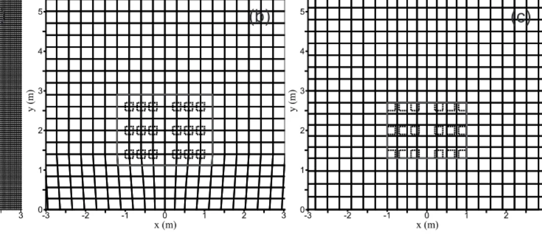
presents the computational meshes used. Note that Fig. 2b corresponds to 1
the gap-conforming mesh required of the anisotropic model (Sanders et al., 2
2008), where vertices are placed at the centroid of obstructions, cells are 3
aligned with pore spaces, and edges intersect constrictions in the pore space. 4
Additionally, Fig. 2c corresponds to a region conforming mesh that precisely 5
circumscribes the subdomain filled with flow barriers (Soares-Fraz˜ao et al., 6
2008; Guinot, 2012). Four variants of the isotropic porosity model are used 7
to account for both mesh designs and two alternative porosity values cor-8
responding to the region-average volumetric porosity Soares-Fraz˜ao et al. 9
(2008) and the areal porosity (Guinot, 2012), as shown in Table 1. It is 10
noted that an REV cannot be rigorously established in this test case due to 11
the anisotropy, heterogeneity and limited spatial extent of the flow barriers, 12
so the assumptions required to apply the isotropic model are not satisfied. 13
However, isotropic models have yielded credible predictions in other applica-14
tions where these requirements were not satisified (Guinot, 2012), motivating 15
further study here. 16
2.6. Definition of Errors 17
Three types of errors are reported: (a) structural model errors, (b) scale 18
errors and (c) porosity model errors. Structural model errors are defined 19
by the difference, as measured by L1 =PNj=1|(w1)j− (w2)j|/N, between the
20
converged CSW prediction and gage measurements of flood depths. Scale er-21
rors are defined by the difference between the CSW (point scale) and CSW-P 22
(pore scale) predictions at gage locations, and are computed for both depth 23
and velocity. Porosity model errors are defined by the difference between 24
porosity model predictions and CSW-P at gage locations (pore scale com-25
parison), and are evaluated for both depth and velocity. 1
2.7. Model Parameterization and Calibration 2
In all seven models, mesh vertex heights were assigned based on reservoir 3
or floodplain bed elevations, and mesh cells were assigned a Nikuradse sand-4
grain roughness height ks to model bottom shear. Further, a no-normal-flux
5
boundary condition was enforced along the reservoir boundaries and concrete 6
wall separating the reservoir and floodplain, and a free-outflow boundary 7
condition was enforced along the remaining three sides of the floodplain. 8
The gate opening was modeled as an instantaneous breach since the time 9
scale of opening (<3 s) is short compared with the time-scale of the breach 10
flow (>100 s). 11
To apply the anisotropic porosity model, the cell-based porosity φj and
12
edge-based porosity ψk were computed based on the intersection of the mesh
13
with the footprint of the solid blocks following previously described methods 14
(Sanders et al., 2008; Schubert and Sanders, 2012). Additionally, the frontal 15
area parameter af required to parameterize drag was computed on a
cell-by-16
cell basis in accordance with the projected area facing the dam as described 17
previously (Sanders et al., 2008). 18
To apply the isotropic porosity models, φj and ψkwere assigned a uniform
19
value inside the block zone as shown in Table 1. Volumetric porosity values 20
used in PSW-I-1A and PSW-I-2A are based on the spatial extent of cells 21
that contact the obstructions, and the porosity values differ slightly based 22
on the mesh. Areal porosity values used in PSW-I-1B and PSW-I-2B are 23
based on the transect E-E’ in Fig. 1d. A uniform frontal area parameter was 24
also specified inside the block zone equal to the total frontal area facing the 25
dam, normalized by the size of the block zone. This corresponds to 0.83 and 1
1.29 m−1 (Table 1) for the meshes shown Fig. 2b and 2c, respectively.
2
Outside the block zone, a porosity value of unity was assigned in all 3
porosity models. Also, the frontal area was set to zero. 4
The roughness parameter, ks, was manually calibrated by applying CSW
5
to the first KICT flow scenario (h0=0.30 m) with ks values ranging from 0.03
6
to 0.3 cm, which is an established range for concrete (Munson et al., 2006). 7
The ks value achieving the best agreement between predicted depths and
8
gage measurements (minimum L1 norm) was subsequently used in all other
9
models and in the second KICT flow scenario (h0=0.45 m).
10
To calibrate co
D, each of the porosity models was applied to the first KICT
11
flow scenario with co
D values ranging from 1.0 to 3.0. This range corresponds
12
to rectangular shaped blocks in an idealized two-dimensional flow (Munson 13
et al., 2006), and it is recognized that co
D may also vary depending on
shel-14
tering effects from the clustering of solid barriers and three-dimensional flow 15
effects (Sanders et al., 2008). Several options deserve consideration as the 16
reference solution for the L1 error norm. Calibration to gage measurements
17
is the first option and is motivated by the goal of minimizing the overall 18
error in the porosity model prediction, whereas another option is calibration 19
to CSW-P predictions which is motivated by the goal of minimizing porosity 20
model errors. Further, calbration to CSW-P depth and/or velocity predic-21
tions is possible. Here, all three options are pursued: calibration to depth 22
measurements, CSW-P predictions of depth at gage locations, and CSW-P 23
predictions of velocity at gage locations. 24
3. Results 1
3.1. Convergence of the CSW model 2
A resolution of 0.05 m was selected for CSW after a convergence check 3
with a 0.025 m mesh of approximately 1.3 million computational cells. This 4
showed that the average convergence error (measured over the simulation 5
period at each gage) of the CSW depth prediction was less than 2 mm at 6
all stations except Gage 2, where the convergence error was found to be 7
6 mm. Over all stations, the average convergence error was approximately 8
1 mm. Gage 2 is located in front of the leading row of obstructions (see 9
Fig. 1). Here, super-critical flow through the breach strikes the first row 10
of blocks, and a bow shock (hydraulic jump) forms across the width of the 11
blocks as shown in Fig. 3. Based on the curvature of the shock wave, Gage 12
2 is on the windward side of the shock and Gages 11 and 18 are on the 13
leeward side. Further, the width of the shock wave (measured in y direction 14
on Fig. 3) is minimal at Gage 2: over a distance of 30 cm in the y direction, 15
the water depth rises up from 5 cm to 16 cm, and then down again to 10 cm, 16
approximately, based on results shown in Fig. 3(b). As the mesh is coarsened 17
from 0.025 to 0.05 m resolution, this narrow band of super-elevated water is 18
diffused slightly and its windward edge moves closer to Gage 2, leading to 19
higher water depth predictions. Hence, the relatively large convergence error 20
at Gage 2 is explained by its position at the leading edge of a shock wave. 21
It is noted that porosity models use a 30 cm mesh resolution (Fig. 2(c) and 22
(d), and Table 1), which is too coarse to sharply resolve the narrow band of 23
super-elevated water at Gage 2. This shows that pore scale and point scale 24
values of flood predictions may differ substantially as a result of localized 25
wakes and wave reflections from flow obstructions. 1
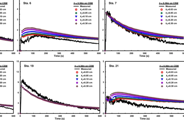
3.2. Calibration of ks
2
Fig. 4 shows CSW model predictions of depth using ksvalues from 0.03 to
3
0.3 cm, compared with measurements for a selection of gages. Additionally, 4
Table 2 shows L1 norms for CSW model. These results demonstrate that the
5
influence of roughness depends on the gage location, but overall roughness 6
does not exhibit a strong influence on the average error. The implication 7
is that momentum losses are dominated by the geometric constriction and 8
form drag associated with the solid blocks, not skin friction from the bottom 9
boundary. All subsequent modeling uses ks=0.03 cm since this leads to the
10
most accurate prediction based on the values considered. 11
3.3. Calibration of co D
12
Table 3 presents L1 norms in porosity model predictions as a function
13 of co
D and different reference solutions. This shows that optimal coD depends
14
on the porosity model and also depends on whether the goal is to minimize 15
total errors or porosity model errors. In four of the five models, minimizing 16
porosity model errors calls for a drag coefficient on the low end of the range 17
(1.0) while minimizing total errors calls for a drag coefficient at the high end 18
of the range (3.0). We conjecture that the goal of a porosity model should 19
be to reproduce as accurately as possible the pore-scale averaged solution of 20
the shallow-water equations, and not necessary match measurements. How-21
ever, the results here clearly indicate that co
D can be tuned to improve the
22
agreement with measurements. 23
The calibration also shows that over a range of physically realistic drag 1
coefficient values, the anisotropic model consistently produces smaller total 2
errors and porosity model errors in flood depths. Further, the anisotropic 3
model performs particularly well with respect to velocity predictions, as the 4
porosity model errors are nearly twice as large for isotropic models versus 5
the anisotropic model. 6
In the analysis of model errors which follows, results of all three cali-7
brations are considered and referenced as Calib1 (measured depth), Calib2 8
(CSW-P depth prediction), and Calib3 (CSW-P velocity prediction). 9
3.4. Model Predictions and Errors 10
Table 4 provides a summary of all model configurations and run times, 11
including optional parameter values corresponding to different calibrations. 12
Models were executed using a 3.07 GHz Intel R
CoreTM i7 CPU with 8GB 13
RAM. The differences in run time are striking as in previous studies. Com-14
pared with CSW, the porosity models execute almost three orders of magni-15
tude faster. 16
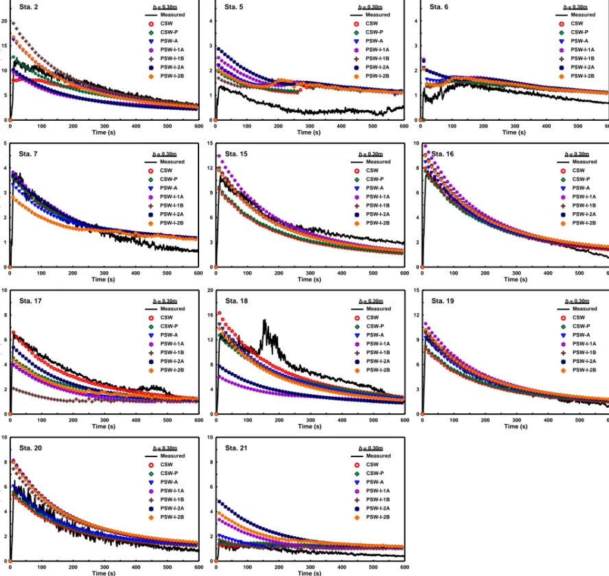
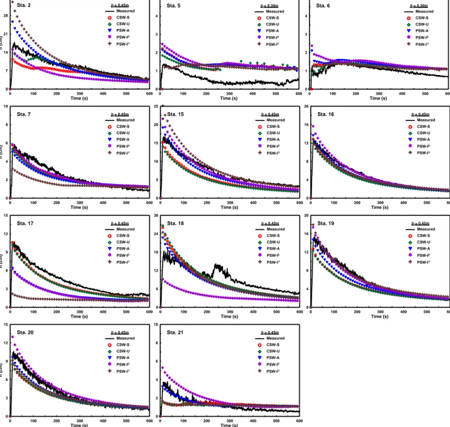
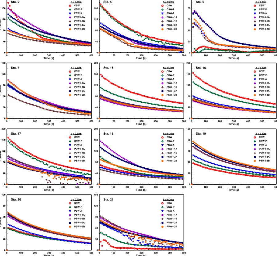
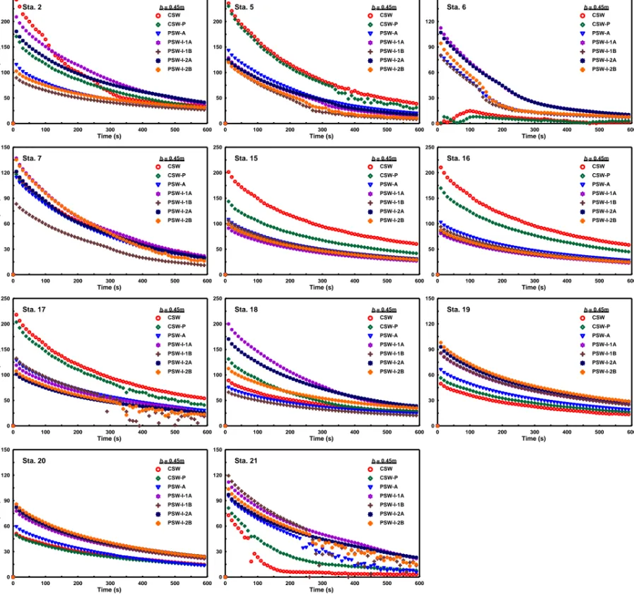
Figs. 5 and 6 present predictions and gage measurements of flood depth 17
for the first (h0=0.30 m) and second (h0=0.45 m) test cases based on Calib1,
18
and Figs. 7 and 8 present model predictions of velocity for the first and 19
second test cases based on Calib1. Results from Calib2 and 3 are not shown 20
graphically, but Table 5 shows L1 norms according to the porosity model,
21
the calibration, and the reference solution. L1 norms based on flood depth
22
measurements are used to measure the structural model error in the CSW 23
model and the total error in the porosity models, while L1 norms based on
24
the CSW-P prediction are used to measure porosity model errors. The scale 25
error is measured by an L1 norm between the CSW and CSW-P predictions.
1
3.4.1. Structural Model Errors 2
The CSW prediction is shown to yield a good approximation of flood 3
depths across the spatial domain (Fig. 5), with an average error of only 0.63 4
cm (Table 5), which represents just 2% of the initial depth in the reservoir. 5
The main limitations of CSW are noted at Sta. 18 where a spurious wave is 6
measured in the experiment that is not explained by the model, and at Sta. 7
5 where the model overpredicts flood depths roughly by a factor of two. In 8
a second test case involving h0=0.45 m (Fig. 6), the average error is 0.89 cm
9
(Table 5) which is again just 2% of the initial depth in the reservoir. Hence, 10
after calibration of the model to the first test case, the model performs with 11
the same relative error in a second test case. 12
3.4.2. Scale Errors 13
Differences between point scale (CSW) predictions and pore-scale (CSW-14
P) predictions of flood depth constitute the scale error which is at least 15
65% smaller than the structural model error according to L1 norms shown
16
in Table 5. In particular, the scale error in depth is 0.18 cm in the first 17
test case where the structural model error is 0.63 cm. In the second test 18
case, the scale error is 0.30 cm while the structural model error is 0.89 cm. 19
Table 5 also shows that the scale error in velocity is 7.45 and 9.12 cm/s, 20
which corresponds to about 2% of the theoretical peak velocity of a dry-bed 21
dam break flood wave, (gh0)1/2.
22
Fig. 5 and 6 illuminate the origin of the scale error. In the first test case 23
(Fig. 5), CSW-P notably departs from CSW at Sta. 2 which is explained 24
by the shock waves shown in Fig. 3. This occurs because at the point scale, 1
the prediction corresponds to one side of the shock or the other, while at the 2
pore scale, the prediction corresponds to a spatial average around the shock. 3
Noticeable differences also occur at two other stations outside perimeter of 4
the obstructions (e.g., Sta. 17 and 18), while differences away from the 5
obstructions (Sta. 5, 6, and 7) and at stations off center from the main flow 6
path (Sta. 19 and 20) are minimal. 7
Differences between the point scale and pore-scale velocities in Fig. 7 8
and 8 are noted at Sta. 2, 15 and 16 where relatively high velocities occur 9
due to the alignment of this channel with the dam-break flood wave. Here, 10
faster velocities occur along the centerline and slower velocities occur near 11
the blocks as a result of wakes, and the monitoring stations sample the fastest 12
moving water. Relatively large scale effects are also noted at Sta. 18 and 21. 13
3.4.3. Porosity Model Errors 14
Attention is now focused on porosity model errors in flood depth and 15
velocity, which are measured by a comparison of porosity model predictions 16
and CSW-P. Table 5 shows that the anistropic porosity model introduces 17
a significantly smaller error in depth and velocity than all of the isotropic 18
porosity models. For example, in the first and second test cases, isotropic 19
model errors in depth were 65-210% and 77-240% greater than the anistropic 20
model, respectively, based on Calib2. Additionally, isotropic model errors in 21
velocity were 83-97% and 80-86% greater than the anistropic model for the 22
first and second test cases, respectively, based on Calib3. Data in Table 5 23
also shows that the magnitude of the porosity model errors is mostly greater 24
than or equal to the scale error, but less than the structural model errors, 25
for both depth and velocity. The exception is the second test case where the 1
anisotropic porosity model errors in depth are actually smaller than the scale 2
error. 3
The total error of the porosity models relative to point-scale predictive 4
skill is also shown in Table 5, with L1 norms based on gage depth
measure-5
ments. The total errors of the anisotropic porosity model are nearly identical 6
to CSW and CSW-P based on Calib1, while all of the isotropic models yield 7
larger total errors. Errors in the isotropic models range from 16 to 59% 8
higher than CSW errors in the first test case, and 2 to 29% higher in the 9
second test case, based on Calib1. 10
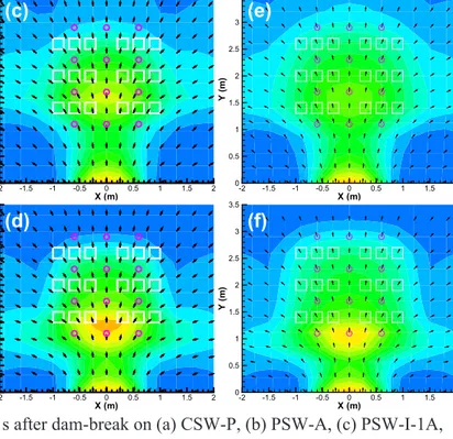
3.5. Spatial Variability 11
Previously shown results reveal at-a-station dynamics, but it is also worth-12
while to examine the spatial structure of flood predictions. For the h0=0.30 m
13
case, Fig. 9 shows contours of pore-scale flood depth and vectors representing 14
the pore scale velocity magnitude and direction 50 s after the dam-break as 15
depicted by: (Fig. 9a) CSW-P model, (Fig. 9b) PSW-A model, and (Fig. 9c-f) 16
the four isotropic porosity models. CSW-P model predicts a zone of elevated 17
water (region colored green, yellow and red) that approximates a triangular 18
shape, and this shape is retained fairly well by PSW-A model, but not as 19
well by the isotropic models. The isotropic models predict a more rounded 20
shape which reflects a lack of directionality. Focusing on the bow shock in 21
front of the obstructions, CSW-P model and PSW-A model predict a lat-22
erally distorted shape, while the isotropic models predict a more rounded 23
shape, again reflecting a lack of directionality. 24
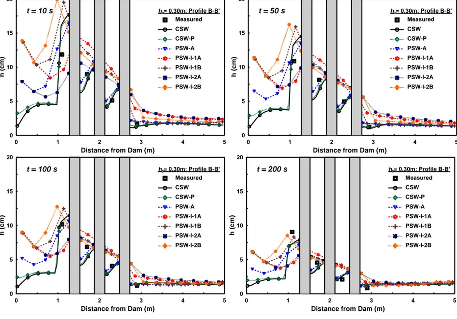
Fig. 10 shows the flood depth distribution for the h0=0.30 m case at four
successive times along the transects through the block zone labeled B-B’ in 1
Fig. 1(c), as depicted by point scale measurements, CSW, CSW-P, and the 2
porosity models. CSW, CSW-P and PSW-A model shows the formation 3
of a bow shock 1 m from the dam and immediately upstream of the first 4
block, and an adverse free surface slope upstream of the second and third 5
block from the dam. On the other hand, the isotropic porosity models fail 6
to capture this depth variability and instead predict a relatively smooth 7
variation of the flood depth through the block zone. This is a result of using 8
a uniform porosity value through the region of obstacles, and consistent with 9
the design of isotropic models to predict flow properties at the REV scale 10
which is considerably larger than the pore scale. Fig. 9 and 10 also reveal 11
insight into the sensitivity of isotropic porosity models to the porosity value. 12
Generally, with a decrease in the porosity value, the height of the bow shock 13
increases and it shifts forwards towards the dam. 14
4. Discussion 15
The preceding results show that porosity model errors may be signif-16
icantly larger than scale errors which poses an opportunity for improved 17
porosity models. The margin for improvement of the anisotropic model rela-18
tive to flood heights is small, but the potential for improvement of the veloc-19
ity predictions is greater and motivates improved models of flow resistance, 20
possibly allowing for more spatial variability in parameters, or even funda-21
mentally new approaches or more advanced calibration procedures. However, 22
research directed at improving porosity model formulations should be mindful 23
of structural model errors. Based on the data presented here, the anisotropic 24
model is equally accurate as the point-scale classical shallow-water model 1
relative to flood depth prediction, so further reduction in porosity model 2
errors cannot be expected to reduce total errors. Broadly, porosity models 3
cannot be expected to predict flood heights any more accurately than the 4
pore-scale average of the foundational flow model, in this case the classical 5
shallow-water equations. 6
There is critical need for urban flood inundation models that can be 7
efficiently applied over practical scales such as a city or regional flood plain, 8
and these results and previous studies (Yu and Lane, 2005; McMillan and 9
Brasington, 2007; Soares-Fraz˜ao and Zech, 2008; Sanders et al., 2008; Guinot, 10
2012) reveal great potential to address this need. But aside from accuracy, 11
another critical question to address is whether any of the porosity models can 12
be more easily parameterized and validated in practical applications. High 13
quality site data is often available for flood modeling studies but calibration 14
data is rare, so there is a need for flood models with parameters that can 15
be estimated deterministically and relied upon to make accurate predictions. 16
This further supports use of the anisotropic model presented here because 17
porosity parameters are a deterministic function of the flow obstructions 18
(Sanders et al., 2008; Schubert and Sanders, 2012), in contrast with the 19
isotropic model where it is unclear how to define a porosity given that a range 20
of values could be used corresponding to volumetric and aerial porosities 21
defined at different spatial scales. However, calibration data may still needed 22
to estimate porosity model drag parameters (e.g., Schubert and Sanders, 23
2012). In the less common scenario where high quality site data are not 24
available to guide the porosity specification, but calibration data exists, the 25
isotropic model may be preferred as the porosity value itself can be used as 1 a calibration parameter. 2 5. Conclusions 3
Urban flood models based on porous shallow-water equations predict 4
flood depths and velocities with three types of errors: (a) structural model er-5
rors associated with the limitations of the 2D shallow-water equations (e.g., 6
hydrostatic pressure, vertical uniform velocity distributions), (b) scale er-7
rors associated with use of a relatively coarse, pore scale grid comparable to 8
the spacing between buildings, and (c) porosity model errors related to the 9
treatment of sub-grid scale obstructions. Results show that in this unique 10
test case with anisotropy in the porosity distribution as in practical appli-11
cations, porosity model errors are mostly greater than scale errors but less 12
than structural model errors, although in one test case the porosity model 13
error of the anisotropic model was slightly less than the scale error. Results 14
also show that porosity model errors in depth and velocity are significantly 15
higher using an isotropic porosity model compared with an anisotropic model, 16
and that the anisotropic porosity model is no less accurate than a fine grid 17
shallow-water model, based on the total error. Recognizing that all porosity 18
models reduced run times by a factor of nearly a thousand compared with 19
the classical shallow-water models, the anistropic porosity model stands out 20
as the most efficient approach for pore-scale modeling based on its low level 21
of error, among models considered here. Additionally, the anistropic poros-22
ity model used here is more successful at resolving pore-scale flow variability 23
than isotropic models because the latter are constrained to scales larger than 24
the REV. 1
Results show that significant differences may exist between pore-scale and 2
point-scale flood conditions in close proximity to flow obstructions, for ex-3
ample due to wave reflections and wakes, so porosity model flood predictions 4
should be used cautiously to inform point-scale flood risk decision-making, 5
such as whether flood heights will rise above the threshold of a door along 6
a roadway. However, results validate the utility of porosity models for map-7
ping flood heights at the pore-scale, i.e., the average flood height across a 8
roadway. 9
Further research into porosity models should be directed at reducing 10
porosity model errors in velocity, for example with improved drag param-11
eterizations, but should be mindful of limitations posed by structural model 12
errors. Finally, the cell averaging of fine-scale classical shallow-water model 13
predictions is found to be an effective approach for gaging the merits of alter-14
native porosity model formulations, as this enables a direct measure of the 15
porosity model error. 16
6. Acknowledgements 17
This work was supported by the MRPI program of the University of Califor-18
nia Office of the President and the Infrastructure Management and Extreme 19
Events program of the National Science Foundation (CMMI-1129730). The 20
authors wish to thank K. Yoon and his research team for their efforts to 21
conduct the laboratory experiments presented here. 22
References 1
References 2
Arega, F., Sanders, B.F., 2004. Dispersion model for tidal wetlands. J. Hy-3
draul. Eng. 130(8), 739–754. 4
Bates, P.D., Horritt, M.S., Fewtrell, T.J., 2010. A simple inertial formulation 5
of the shallow water equations for efficient two-dimensional flood inunda-6
tion modelling. J. Hydrol. 387, 33–45. 7
Bates, P.D., 2012. Integrating remote sensing data with flood inundation 8
models: how far have we got? Hydrol. Process. 26, 2515–2521. 9
Bear, J., 1988 Dynamics of Fluids in Porous Media, Second Edition (of the 10
1972 book) Dover Publ., New York, 761p. 11
Begnudelli, L., Sanders, B.F., Bradford, S.F., 2008. An adaptive Godunov-12
based model for flood simulation. J. Hydraul. Eng. 134(6), 714–725. 13
Cea, L., V´azquez-Cend´on, M.E., 2010. Unstructured finite volume discretiza-14
tion of two-dimensional depth-averaged shallow water equations with 15
porosity. Int. J. Num. Meth. Fluid. 63, 903–930. 16
Chen, A., Evans, B., Djordjevi´c, S., Savi´c, D.A., 2012. A coarse-grid ap-17
proach to represent building blockage effects in 2D urban flood modelling, 18
J. Hydrol. 426–427, 1–16. 19
Defina, A., 2000. Two-dimensional shallow flow equations for partially dry 20
areas. Water Resour. Res. 36(11), 3251–3264. 21
Guinot, V., 2012. Multiple porosity shallow water models for macroscopic 1
modelling of urban floods. Adv. Water Resour. 37, 40–72. 2
Haaland, S.E., 1983. Simple and explicit formulas for the friction factor in 3
turbulent pipe flow. J. Fluids Eng. 105(1), 89–90. 4
Kim, B., Sanders, B.F., Schubert, J.E., Famiglietti, J.S., 2014. Mesh type 5
tradeoffs in 2D hydrodynamic modeling of flooding with a Godunov-based 6
flow solver. Adv. Water Resour. 68, 42–61. 7
McMillan, H.K., Brasington, J., 2007. Reduced complexity strategies for 8
modelling urban floodplain inundation. Geomorphology 90, 226–243. 9
Munson, B.R., Young, D.F., Okiishi, T.H., 2006. Fundamentals of fluid me-10
chanics, 5th ed., John Wiley & Sons, 769p. 11
Nepf, H.M., 1999. Drag, turbulence and diffusion in flow through emergent 12
vegetation. Water Resour. Res. 35(2), 479–489. 13
Sampson, C.C., Fewtrell, T.J., Duncan, A., Shaad, K., Horritt, M.S., Bates, 14
PD., 2012. Use of terrestrial laser scanning data to derive decimetric res-15
olution urban inundation models. Adv. Water Resour. 41, 1–17. 16
Sanders, B.F., 2008. Integration of a shallow-water model with a local time 17
step. J. Hydraul. Res. 46(8), 466–475. 18
Sanders, B.F., Schubert, J.E., Gallegos, H.A., 2008. Integral formulation of 19
shallow-water equations with anisotropic porosity for urban flood model-20
ing. J. Hydrol. 362, 19–38. 21
Schubert, J.E., Sanders, B.F., 2012. Building treatments for urban flood 1
inundation models and implications for predictive skill and modeling effi-2
ciency. Adv. Water Resour. 41, 49–64. 3
Soares-Fraz˜ao, S., Lhomme, J., Guinot, V., Zech, Y., 2008. Two-dimensional 4
shallow-water model with porosity for urban flood modelling. J. Hydraul. 5
Res. 46(1), 45–64. 6
Soares-Fraz˜ao, S., Zech, Y., 2008. Dam-break flow through an idealized city. 7
J. Hydraul. Res. 46(5), 648–658. 8
Stelling, G.S., 2012. Quadtree flood simulations with sub-grid digital eleva-9
tion models. Proc. Inst. Civ. Eng.-Water Manag. 165(10), 567–580. 10
Testa, G., Zuccala, D., Alcrudo, F., Mulet, J., Soares-Fraz˜ao, S., 2007. Flash 11
flood flow experiment in a simplified urban district. J. Hydraul. Res. 45(Ex-12
tra Issue), 37–44. 13
Yoon, K., 2007. Experimental study on flood inundation considering urban 14
characteristics (FFC06-05). Urban Flood Disaster Management Research 15
Center, Seoul. 16
Yu, D., Lane, S.N., 2005. Urban fluvial flood modelling using a two dimen-17
sional diffusion-wave treatment, part 2: development of a sub-grid-scale 18
treatment. Hydrol. Process. 20(7), 1567–1583. 19
Captions of Figures 1
• Fig. 1. Experiment set-up of Yoon (Yoon, 2007): (a) Plan view, (b) 2
Side view, and (c) Close-up of greyed section in Fig. 1(a); and (d) Cell-3
based porosity φ exhibits heterogeneity depending on control volume 4
placement, a vs. b, and edge-based porosities ψ exhibit heterogeneity 5
and anisotropy depending on the chosen transect. 6
• Fig. 2. Computational mesh for (a) CSW and CSW-P, (b) PSW-A, 7
PSW-I-2A and PSW-I-2A, and (c) PSW-I-1A and PSW-I-1B. 8
• Fig. 3. Contours of water depth 50 s after dam-break on CSW-S with 9
(a) 0.05 m and (b) 0.025 m resolution. Vectors indicate velocity direc-10
tion. 11
• Fig. 4. Flood depth sensitivity to roughness height (ks) on CSW.
12
• Fig. 5. Comparison of predicted flood depth and measurement for 13
h0=0.30 m.
14
• Fig. 6. Comparison of predicted flood depth and measurement for 15
h0=0.45 m.
16
• Fig. 7. Comparison of predicted flood velocity for h0=0.30 m.
17
• Fig. 8. Comparison of predicted flood velocity for h0=0.45 m.
18
• Fig. 9. Contours of water depth 50 s after dam-break on (a) CSW-19
P, (b) PSW-A, (c) PSW-I-1A, (d) PSW-I-1B, (e) PSW-I-2A and (f) 20
PSW-I-2B. Vectors indicate velocity direction. 21
• Fig. 10. Profile of flood depth after dam-break for h0=0.30 m at B-B’in
1
Fig. 1(c). 2
Captions of Tables 1
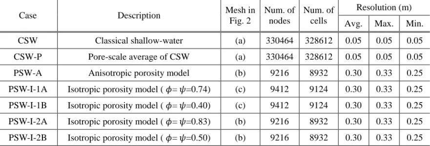
• Table 1. Shallow-water model formulations and corresponding meshes 2
shown in Fig. 2. 3
• Table 2. L1 norms of flood depth for calibration of roughness height
4
(ks) on CSW (unit: cm).
5
• Table 3. L1norms of flood depth for calibration of drag coefficient (coD)
6
on PSW-A and PSW-I. 7
• Table 4. Model parameters and run time. 8
• Table 5. L1 norms of flood depth and velocity based on calibration and
9
reference solution. 10
x (m) y (m ) -3 -2 -1 0 1 2 3 0 1 2 3 4 5 (a) x (m) y (m ) -3 -2 -1 0 1 2 3 0 1 2 3 4 5 (c) x (m) y (m ) -3 -2 -1 0 1 2 3 0 1 2 3 4 5 (b)
Fig. 3. Computational mesh for (a) CSW and CSW-P, (b) PSW-A, PSW-I-2A and PSW-I-2B, and
X (m) Y (m ) -2 -1.5 -1 -0.5 0 0.5 1 1.5 2 0 0.5 1 1.5 2 2.5 3 3.5 0.16 0.15 0.14 0.13 0.12 0.11 0.10 0.09 0.08 0.07 0.06 0.05 0.04 0.03 0.02 0.01 h (m) X (m) Y (m ) -2 -1.5 -1 -0.5 0 0.5 1 1.5 2 0 0.5 1 1.5 2 2.5 3 3.5 0.16 0.15 0.14 0.13 0.12 0.11 0.10 0.09 0.08 0.07 0.06 0.05 0.04 0.03 0.02 0.01 h (m)
Fig. 3. Contours of water depth 50 s after dam-break on CSW with (a) 0.05 m and
(a) (b)
0 100 200 300 400 500 600 Time (s) 0 3 6 9 12 15 h ( c m ) h0= 0.30m on CSW Measured ks=0.03 cm ks=0.05 cm ks=0.10 cm ks=0.20 cm ks=0.30 cm Sta. 2 0 100 200 300 400 500 600 Time (s) 0 1 2 3 4 5 h0= 0.30m on CSW Measured ks=0.03 cm ks=0.05 cm ks=0.10 cm ks=0.20 cm ks=0.30 cm Sta. 6 0 100 200 300 400 500 600 Time (s) 0 1 2 3 4 5 h0= 0.30m on CSW Measured ks=0.03 cm ks=0.05 cm ks=0.10 cm ks=0.20 cm ks=0.30 cm Sta. 7 0 100 200 300 400 500 600 Time (s) 0 2 4 6 8 10 h ( c m ) h0= 0.30m on CSW Measured ks=0.03 cm ks=0.05 cm ks=0.10 cm ks=0.20 cm ks=0.30 cm Sta. 16 0 100 200 300 400 500 600 Time (s) 0 3 6 9 12 15 h0= 0.30m on CSW Measured ks=0.03 cm ks=0.05 cm ks=0.10 cm ks=0.20 cm ks=0.30 cm Sta. 19 0 100 200 300 400 500 600 Time (s) 0 1 2 3 4 5 h0= 0.30m on CSW Measured ks=0.03 cm ks=0.05 cm ks=0.10 cm ks=0.20 cm ks=0.30 cm Sta. 21
Fig. 4. Flood depth sensitivity to roughness height (ks) on CSW.
0 100 200 300 400 500 600 Time (s) 0 5 10 15 20 25 h ( c m ) h0= 0.30m Measured CSW CSW-P PSW-A PSW-I-1A PSW-I-1B PSW-I-2A PSW-I-2B Sta. 2 0 100 200 300 400 500 600 Time (s) 0 1 2 3 4 5 h0= 0.30m Measured CSW CSW-P PSW-A PSW-I-1A PSW-I-1B PSW-I-2A PSW-I-2B Sta. 5 0 100 200 300 400 500 600 Time (s) 0 1 2 3 4 5 h0= 0.30m Measured CSW CSW-P PSW-A PSW-I-1A PSW-I-1B PSW-I-2A PSW-I-2B Sta. 6 0 100 200 300 400 500 600 Time (s) 0 1 2 3 4 5 h ( c m ) h0= 0.30m Measured CSW CSW-P PSW-A PSW-I-1A PSW-I-1B PSW-I-2A PSW-I-2B Sta. 7 0 100 200 300 400 500 600 Time (s) 0 3 6 9 12 15 h0= 0.30m Measured CSW CSW-P PSW-A PSW-I-1A PSW-I-1B PSW-I-2A PSW-I-2B Sta. 15 0 100 200 300 400 500 600 Time (s) 0 2 4 6 8 10 h0= 0.30m Measured CSW CSW-P PSW-A PSW-I-1A PSW-I-1B PSW-I-2A PSW-I-2B Sta. 16 0 100 200 300 400 500 600 Time (s) 0 2 4 6 8 10 h ( c m ) h0= 0.30m Measured CSW CSW-P PSW-A PSW-I-1A PSW-I-1B PSW-I-2A PSW-I-2B Sta. 17 0 100 200 300 400 500 600 Time (s) 0 4 8 12 16 20 h0= 0.30m Measured CSW CSW-P PSW-A PSW-I-1A PSW-I-1B PSW-I-2A PSW-I-2B Sta. 18 0 100 200 300 400 500 600 Time (s) 0 3 6 9 12 15 h0= 0.30m Measured CSW CSW-P PSW-A PSW-I-1A PSW-I-1B PSW-I-2A PSW-I-2B Sta. 19 0 100 200 300 400 500 600 Time (s) 0 2 4 6 8 10 h ( c m ) h0= 0.30m Measured CSW CSW-P PSW-A PSW-I-1A PSW-I-1B PSW-I-2A PSW-I-2B Sta. 20 0 100 200 300 400 500 600 Time (s) 0 2 4 6 8 10 h0= 0.30m Measured CSW CSW-P PSW-A PSW-I-1A PSW-I-1B PSW-I-2A PSW-I-2B Sta. 21
Fig. 5. Comparison of predicted flood depth and measurement for h0=0.30 m.
0 100 200 300 400 500 600 Time (s) 0 7 14 21 28 35 h ( c m ) h0= 0.45m Measured CSW-S CSW-U PSW-A PSW-I PSW-I Sta. 2 0 100 200 300 400 500 600 Time (s) 0 1 2 3 4 5 h0= 0.30m Measured CSW-S CSW-U PSW-A PSW-I PSW-I Sta. 5 0 100 200 300 400 500 600 Time (s) 0 1 2 3 4 5 h0= 0.30m Measured CSW-S CSW-U PSW-A PSW-I PSW-I Sta. 6 0 100 200 300 400 500 600 Time (s) 0 2 4 6 8 10 h ( c m ) h0= 0.45m Measured CSW-S CSW-U PSW-A PSW-I PSW-I Sta. 7 0 100 200 300 400 500 600 Time (s) 0 5 10 15 20 25 h0= 0.45m Measured CSW-S CSW-U PSW-A PSW-I PSW-I Sta. 15 0 100 200 300 400 500 600 Time (s) 0 4 8 12 16 20 h0= 0.45m Measured CSW-S CSW-U PSW-A PSW-I PSW-I Sta. 16 0 100 200 300 400 500 600 Time (s) 0 3 6 9 12 15 h ( c m ) h0= 0.45m Measured CSW-S CSW-U PSW-A PSW-I PSW-I Sta. 17 0 100 200 300 400 500 600 Time (s) 0 6 12 18 24 30 h0= 0.45m Measured CSW-S CSW-U PSW-A PSW-I PSW-I Sta. 18 0 100 200 300 400 500 600 Time (s) 0 4 8 12 16 20 h0= 0.45m Measured CSW-S CSW-U PSW-A PSW-I PSW-I Sta. 19 0 100 200 300 400 500 600 Time (s) 0 3 6 9 12 15 h ( c m ) h0= 0.45m Measured CSW-S CSW-U PSW-A PSW-I PSW-I Sta. 20 0 100 200 300 400 500 600 Time (s) 0 2 4 6 8 10 h0= 0.45m Measured CSW-S CSW-U PSW-A PSW-I PSW-I Sta. 21
Fig. 6. Comparison of predicted flood depth and measurement for h0=0.45 m.
0 100 200 300 400 500 600 Time (s) 0 40 80 120 160 200 V ( c m /s ) h0= 0.30m CSW CSW-P PSW-A PSW-I-1A PSW-I-1B PSW-I-2A PSW-I-2B Sta. 2 0 100 200 300 400 500 600 Time (s) 0 40 80 120 160 200 h0= 0.30m CSW CSW-P PSW-A PSW-I-1A PSW-I-1B PSW-I-2A PSW-I-2B Sta. 5 0 100 200 300 400 500 600 Time (s) 0 20 40 60 80 100 h0= 0.30m CSW CSW-P PSW-A PSW-I-1A PSW-I-1B PSW-I-2A PSW-I-2B Sta. 6 0 100 200 300 400 500 600 Time (s) 0 30 60 90 120 150 V ( c m /s ) h0= 0.30m CSW CSW-P PSW-A PSW-I-1A PSW-I-1B PSW-I-2A PSW-I-2B Sta. 7 0 100 200 300 400 500 600 Time (s) 0 40 80 120 160 200 h0= 0.30m CSW CSW-P PSW-A PSW-I-1A PSW-I-1B PSW-I-2A PSW-I-2B Sta. 15 0 100 200 300 400 500 600 Time (s) 0 40 80 120 160 200 h0= 0.30m CSW CSW-P PSW-A PSW-I-1A PSW-I-1B PSW-I-2A PSW-I-2B Sta. 16 0 100 200 300 400 500 600 Time (s) 0 40 80 120 160 200 V ( c m /s ) h0= 0.30m CSW CSW-P PSW-A PSW-I-1A PSW-I-1B PSW-I-2A PSW-I-2B Sta. 17 0 100 200 300 400 500 600 Time (s) 0 40 80 120 160 200 h0= 0.30m CSW CSW-P PSW-A PSW-I-1A PSW-I-1B PSW-I-2A PSW-I-2B Sta. 18 0 100 200 300 400 500 600 Time (s) 0 20 40 60 80 100 h0= 0.30m CSW CSW-P PSW-A PSW-I-1A PSW-I-1B PSW-I-2A PSW-I-2B Sta. 19 0 100 200 300 400 500 600 Time (s) 0 20 40 60 80 100 V ( c m /s ) h0= 0.30m CSW CSW-P PSW-A PSW-I-1A PSW-I-1B PSW-I-2A PSW-I-2B Sta. 20 0 100 200 300 400 500 600 Time (s) 0 30 60 90 120 150 h0= 0.30m CSW CSW-P PSW-A PSW-I-1A PSW-I-1B PSW-I-2A PSW-I-2B Sta. 21
Fig. 7. Comparison of predicted velocity for h0=0.30 m.
0 100 200 300 400 500 600 Time (s) 0 50 100 150 200 250 V ( c m /s ) h0= 0.45m CSW CSW-P PSW-A PSW-I-1A PSW-I-1B PSW-I-2A PSW-I-2B Sta. 2 0 100 200 300 400 500 600 Time (s) 0 50 100 150 200 250 h0= 0.45m CSW CSW-P PSW-A PSW-I-1A PSW-I-1B PSW-I-2A PSW-I-2B Sta. 5 0 100 200 300 400 500 600 Time (s) 0 30 60 90 120 150 h0= 0.45m CSW CSW-P PSW-A PSW-I-1A PSW-I-1B PSW-I-2A PSW-I-2B Sta. 6 0 100 200 300 400 500 600 Time (s) 0 30 60 90 120 150 V ( c m /s ) h0= 0.45m CSW CSW-P PSW-A PSW-I-1A PSW-I-1B PSW-I-2A PSW-I-2B Sta. 7 0 100 200 300 400 500 600 Time (s) 0 50 100 150 200 250 h0= 0.45m CSW CSW-P PSW-A PSW-I-1A PSW-I-1B PSW-I-2A PSW-I-2B Sta. 15 0 100 200 300 400 500 600 Time (s) 0 50 100 150 200 250 h0= 0.45m CSW CSW-P PSW-A PSW-I-1A PSW-I-1B PSW-I-2A PSW-I-2B Sta. 16 0 100 200 300 400 500 600 Time (s) 0 50 100 150 200 250 V ( c m /s ) h0= 0.45m CSW CSW-P PSW-A PSW-I-1A PSW-I-1B PSW-I-2A PSW-I-2B Sta. 17 0 100 200 300 400 500 600 Time (s) 0 50 100 150 200 250 h0= 0.45m CSW CSW-P PSW-A PSW-I-1A PSW-I-1B PSW-I-2A PSW-I-2B Sta. 18 0 100 200 300 400 500 600 Time (s) 0 30 60 90 120 150 h0= 0.45m CSW CSW-P PSW-A PSW-I-1A PSW-I-1B PSW-I-2A PSW-I-2B Sta. 19 0 100 200 300 400 500 600 Time (s) 0 30 60 90 120 150 V ( c m /s ) h0= 0.45m CSW CSW-P PSW-A PSW-I-1A PSW-I-1B PSW-I-2A PSW-I-2B Sta. 20 0 100 200 300 400 500 600 Time (s) 0 30 60 90 120 150 h0= 0.45m CSW CSW-P PSW-A PSW-I-1A PSW-I-1B PSW-I-2A PSW-I-2B Sta. 21
Fig. 8. Comparison of predicted velocity for h0=0.45 m.
X (m) Y (m ) -2 -1.5 -1 -0.5 0 0.5 1 1.5 2 0 0.5 1 1.5 2 2.5 3 3.5 0.16 0.15 0.14 0.13 0.12 0.11 0.10 0.09 0.08 0.07 0.06 0.05 0.04 0.03 0.02 0.01 h (m) X (m) Y (m ) -2 -1.5 -1 -0.5 0 0.5 1 1.5 2 0 0.5 1 1.5 2 2.5 3 3.5 X (m) Y (m ) -2 -1.5 -1 -0.5 0 0.5 1 1.5 2 0 0.5 1 1.5 2 2.5 3 3.5 X (m) Y (m ) -2 -1.5 -1 -0.5 0 0.5 1 1.5 2 0 0.5 1 1.5 2 2.5 3 3.5 X (m) Y (m ) -2 -1.5 -1 -0.5 0 0.5 1 1.5 2 0 0.5 1 1.5 2 2.5 3 3.5 X (m) Y (m ) -2 -1.5 -1 -0.5 0 0.5 1 1.5 2 0 0.5 1 1.5 2 2.5 3 3.5 (a)
Fig. 10. Contours of water depth 50 s after dam-break on (a) CSW-P, (b) PSW-A, (c) PSW-I-1A, (b) (c) (d) (e) (f) Fig.9
0 1 2 3 4 5
Distance from Dam (m)
0 5 10 15 20 h ( c m ) h0= 0.30m: Profile B-B' Measured CSW CSW-P PSW-A PSW-I-1A PSW-I-1B PSW-I-2A PSW-I-2B t = 10 s 0 1 2 3 4 5
Distance from Dam (m)
0 5 10 15 20 h ( c m ) h0= 0.30m: Profile B-B' Measured CSW CSW-P PSW-A PSW-I-1A PSW-I-1B PSW-I-2A PSW-I-2B t = 50 s 0 1 2 3 4 5
Distance from Dam (m)
0 5 10 15 20 h ( c m ) h0= 0.30m: Profile B-B' Measured CSW CSW-P PSW-A PSW-I-1A PSW-I-1B PSW-I-2A PSW-I-2B t = 100 s 0 1 2 3 4 5
Distance from Dam (m)
0 5 10 15 20 h ( c m ) h0= 0.30m: Profile B-B' Measured CSW CSW-P PSW-A PSW-I-1A PSW-I-1B PSW-I-2A PSW-I-2B t = 200 s
Fig. 9. Profile of flood depth after dam-break for h0=0.30 m at B-B’ in Fig. 1(c).
Table 1. Shallow-water model formulations and corresponding meshes shown in Fig. 2
Case Description Mesh in
Fig. 2 Num. of nodes Num. of cells Resolution (m) Avg. Max. Min. CSW Classical shallow-water (a) 330464 328612 0.05 0.05 0.05 CSW-P Pore-scale average of CSW (a) 330464 328612 0.05 0.05 0.05 PSW-A Anisotropic porosity model (b) 9216 8932 0.30 0.33 0.25 PSW-I-1A Isotropic porosity model ( 𝜙= 𝜓=0.74) (c) 9412 9124 0.30 0.33 0.25 PSW-I-1B Isotropic porosity model ( 𝜙= 𝜓=0.40) (c) 9412 9124 0.30 0.33 0.25 PSW-I-2A Isotropic porosity model ( 𝜙= 𝜓=0.83) (b) 9216 8932 0.30 0.33 0.25 PSW-I-2B Isotropic porosity model ( 𝜙= 𝜓=0.50) (b) 9216 8932 0.30 0.33 0.25
Table1
Table 2. L1 norms of flood depth for calibration of roughness height (ks) on CSW (unit: cm).
Case ks
(cm)
Gages inside block zone Gages outside block zone Entire Avg. 2 11&18 12&19 13&20 14&21 15 16 17 Avg. 3&7 4&6 5 Avg.
CSW 0.03 1.08 1.22 0.66 0.44 0.58 1.49 0.23 0.29 0.75 0.33 0.39 0.81 0.51 0.63 0.05 0.94 1.23 0.66 0.44 0.62 1.49 0.23 0.29 0.74 0.35 0.44 0.82 0.54 0.64 0.10 0.71 1.24 0.66 0.44 0.70 1.48 0.23 0.29 0.72 0.40 0.53 0.89 0.61 0.66 0.20 0.56 1.25 0.66 0.45 0.83 1.46 0.23 0.30 0.72 0.49 0.66 1.03 0.72 0.72 0.30 0.57 1.26 0.67 0.46 0.91 1.44 0.23 0.30 0.73 0.56 0.74 1.12 0.81 0.77 Table2