Advertising in a Competitive Market: The Role of Product
Standards, Customer Learning, and Switching Costs
The MIT Faculty has made this article openly available.
Please share
how this access benefits you. Your story matters.
Citation
Anderson, Eric T., and Duncan Simester. “Advertising in a
Competitive Market: The Role of Product Standards, Customer
Learning, and Switching Costs.” Journal of Marketing Research 50,
no. 4 (August 2013): 489–504.
As Published
http://dx.doi.org/10.1509/jmr.11.0538
Publisher
American Marketing Association
Version
Original manuscript
Citable link
http://hdl.handle.net/1721.1/90833
Terms of Use
Creative Commons Attribution-Noncommercial-Share Alike
Detailed Terms
http://creativecommons.org/licenses/by-nc-sa/4.0/
Advertising in a Competitive Market:
The Role of Product Standards, Customer Learning and
Switching Costs
*May 2013
Eric T. Anderson
Northwestern University
Duncan Simester
MIT Sloan School of Management
Standard models of competition predict that firms will sell less when competitors target their customers with advertising. This is particularly true in mature markets with many competitors selling relatively
undifferentiated products. We present findings from a large-scale randomized field experiment that contrast sharply with this prediction. The field experiment measures the impact of competitors’ advertising on sales at a private label retailer of apparel, home furnishings and sporting goods. Surprisingly, for a substantial segment of customers the competitors’ advertisements increased sales at this retailer. This is a robust effect, obtained through experimental manipulation and measuring actual purchases by large samples of randomly assigned customers. The effect is also large with customers ordering over 4% more items in some categories in the Treatment condition (compared to the control). We compare how these positive spillovers vary across product categories to illustrate the importance of product standards, customer learning, and switching costs. The findings have the potential to change our understanding of competition in mature markets.
Keywords: advertising, product standards, customer learning, switching costs
* We thank our research assistant Hojin Jung for his contribution to this work. This paper has benefitted from seminar participants at the 2010 Yale Customer Insights Conference, and the 2011 Yale Marketing Industrial Organization Conference, together with audiences at the following universities: Alberta, Berkeley, Carnegie-Mellon, MIT, and Wisconsin.
1 | P a g e
1.
Introduction
We report the findings from a large scale field experiment to investigate the impact of advertising in a competitive market. The field experiment was conducted with the cooperation of a large national retailer that sells private label apparel, home furnishings and sporting goods. Although we cannot reveal the identity of the retailer, for ease of exposition we will label it “Retail World”. In the field experiment approximately 370,000 of Retail World’s past customers were randomly assigned
The field experiment takes advantage of a common direct-mail practice: sharing of customer information between competing retailers. Sharing is often done on a reciprocal basis, so that firms exchange information for an equivalent number of customers. Firms use this information to identify where to send direct mail advertising, and this provides a unique opportunity to design a field experiment to measure the impact of competitors’ advertising on a firm’s sales. We measure this impact by comparing purchases at Retail World between the two experimental conditions using 20-months of transactions. This period encompasses the twelve month treatment period and eight subsequent months, and includes over one million orders and almost $100 million in Retail World revenue.
to two experimental conditions. The 185,000 customers in the Treatment condition received over 1.1 million targeted direct mail advertisements from Retail World’s close competitors. Most of these
advertisements consisted of competing catalogs containing product information, prices and images for hundreds of products. Customers in the Control condition did not receive these advertisements.
Surprisingly, we find that for a substantial segment of customers the competitors’ advertisements increased sales at Retail World. This effect is large and it is obtained through comparison of actual purchases by large samples of randomly assigned customers. What makes the outcome particularly surprising is that the apparel, home furnishings and sporting goods categories are mature and comprised of many retailers selling relatively undifferentiated products.1
The size of the positive spillovers varied across customers. The largest increase in Retail World sales was from customers who had not made a recent Retail World purchase. The effect also varied across product categories. To explain these positive spillovers and the variation across both categories and customers
The maturity of the markets ensures that all customers are aware of the product categories. Customers can easily search and purchase products at competing firms, customers do not have to learn how to use the products, and compatibility between products is generally not specific to a firm. These are product categories in which we might expect the threat from competition to be particularly strong. Yet, we find positive spillovers from the competitors’ advertising.
1 The US retail apparel market contributes almost 3% of the US gross domestic product. In 2007 customers in the US purchased approximately 20.1 billion garments and 2.4 billion pairs of shoes, representing approximately $371 billion in revenue (AAFA 2008). Sales of apparel and shoes are particularly strong in catalog and Internet channels. The Direct Marketing Association (DMA 2006) reports that the apparel category has a higher volume of Internet and catalog orders than any other product category. In 2006 approximately 32% of US adults ordered an item of apparel from a direct retailer (including 23% of males and 40% of females). Moreover, fully 24% of the 100 largest catalog retailers sell apparel. Not surprisingly, almost all major apparel retailers now use direct mail advertising and catalog and Internet channels to complement their traditional retail stores.
2 | P a g e we will distinguish between the decision to make a purchase in a category, and the selection of which retailer to purchase from. Competitors’ advertising may influence the first decision by priming customers to think about the category. However, even though the need to purchase may have been primed by competitors’ advertising, some customers returned to Retail World to satisfy this need. The focus of the paper is on the choice of which retailer to purchase from. In preliminary interviews for this research some customers described examples of products that they only buy from the Retail World because they have learned which sizes fit. One customer described how he had mailed an outline of his foot to Retail World, which the company used to determine his appropriate size. When he orders Retail World footwear he believes it will fit. However, he also knows that sizing differs across brands and so he avoids buying footwear elsewhere. A key feature of this example is the standardization of product sizes. While footwear sizes are standardized within Retail World’s (private label) brand, they are different from sizes at competing brands.2
Standardization in sizes does not extend to all categories. For example, swimwear sizes are not
standardized even within Retail World’s brand. Customers may need a size 8 when purchasing one style of Retail World swimwear and a size 10 when purchasing another style. As a result the fit of past swimwear purchases may not help predict the fit of a new swimsuit. We will show that variation in how much customers learn about sizes from past purchases helps to explain where the impact from the competitors’ advertising was largest.
If sizes were standardized across all brands, this customer could use Retail World’s size information to also order from other retailers.
While the customer interviews yielded useful initial insights, formally documenting these effects required that we construct measures of how much customers learn from past purchases. Fortunately this market provides an ideal measure of customer learning: changes in customer return rates. The main reason that customers return items is due to concerns about product fit. We compare the response to the competitors’ advertising with the change in return rates between customers’ first and last orders in the category. We find a clear relationship: categories with the larger decreases in return rates due to poor fit are the categories with the most positive treatment effects in the competitive advertising experiment. Across the 35 largest categories, the pair-wise correlation between the Change
in Return Rates and the response to the competitors’ advertising is -0.41 (the rank-order correlation is
-0.50). We interpret this as evidence that learning about product sizes created switching costs in favor of Retail World. These switching costs led customers to purchase from Retail World, even though their need to purchase was primed by the competitors.
Related Literature
Spillover effects have often been studied using Feldman and Lynch’s (1988) accessibility-diagnosticity framework. This theory predicts that “an earlier response will be used as a basis for another subsequent response if the former is accessible and if it is perceived to be more diagnostic than other accessible inputs” (at page 421). In our application, products are associated through a network that includes both retail brands and categories. A retail advertisement may activate the retail brand, a category need and in-turn competing retail brands. This model has been used to explain both positive and negative spillovers among competing brands. For example, Janakiraman, Sismeiro and Dutta (2009) develop an
3 | P a g e empirical framework to investigate positive spillovers between competing brands in the pharmaceutical industry. They find that customers’ quality beliefs about the first entrant can influence customers’ prior beliefs about the quality of later entrants, but only if the products are similar. They do not find any evidence of positive spillovers through advertising. In particular, physicians do not appear to use detailing activities for one drug to form quality perceptions of competing drugs.
Examples of positive advertising spillovers have been established in the context of umbrella brands (among non-competing brands). For example, Balachander and Ghose (2003) show that these positive spillovers may not only project from the parent brand to the brand extension, but that reciprocal spillovers may also operate in the opposite direction (see also Morrin 1999).
Negative spillovers among competing brands have also been documented. Roehm and Tybout (2006, 2009) demonstrate how a product scandal may spillover from a brand like Vioxx, which was recalled due to safety concerns, to damage a competing brand like Celebrex. Analogously, Dark and Richie (2007) illustrate how deceptive advertising can have negative consequences for firms who are unrelated to the original deception. Our findings contribute to our understanding of spillovers by documenting both the existence of positive advertising spillovers between competing brands, and highlighting the moderating role of consumer switching costs.
Our findings also contribute to an extensive literature establishing the existence of state dependencies (consumer loyalty) in consumer choice (Dubé, Hitsch, Rossi and Vitorino 2008; Erdem 1996; Keane 1997; and Seetharaman, Ainslie and Chintagunta 1999). Switching costs represent an important potential source of state dependence. The earliest papers in the switching cost literature assumed that switching costs were exogenous and common across firms. Under these conditions switching costs tend to reduce competition and increase profits in equilibrium (Klemperer 1987). More recently it has been recognized that switching costs may be endogenous. For example, Bergemann and Välimäki (1996) endogenize switching costs in a multi-armed bandit problem in which buyers learn about product quality through experience. If firms can control the level of switching costs we might expect that they would prefer to increase them in order to dampen competition. However, the literature often predicts the opposite result. Anticipation that high switching costs leads will lead to higher second-period profits induces firms to compete aggressively in the first period. If the resulting price competition erodes profits, then firms may reduce switching costs to dampen first-period competition (see for example Caminal and Matutes 1990, Marinoso 2001, Bouckaert and Hans Degryse 2004, and Cabral and Villas-Boas 2005). These distinct goals of “investing” to capture sticky customers and “harvesting” the surplus from them once captured makes it difficult to predict whether the presence of switching costs will increase or decrease the intensity of competition. This has led to recent empirical research evaluating the
contrasting predictions. Dubé, Hitsch and Rossi (2009) provide a prominent recent example. They study the refrigerated orange juice and margarine categories and report that the presence of switching costs can act to amplify the intensity of competition in these grocery markets. Their study focuses on price competition among heterogenous firms and they find that intermediate levels of switching costs may lead to lower prices. When switching costs are much larger, their numerical simulations show that prices can rise as competition is dampened.
Our findings complement these results by extending our understanding of how switching costs impact competitive intensity. The standard result in this context is that large switching costs create lock-in that insulates customers from competitors’ actions. The surprise in our findings is that in the presence of
4 | P a g e switching costs competitors’ actions can generate positive spillovers that are large enough to outweigh competitive substitution. Moreover, the extant switching cost literature has largely focused on price competition in markets for low-involvement fast-moving consumer goods, while we focus on
competitive advertising in markets for higher-priced consumer durables.
Dubé, Hitsch and Rossi (2009) attribute the state dependence in their study to a “psychological” switching cost, including cognitive dissonance in which customers change their preferences to rationalize previous choices. Elsewhere the literature has distinguished between “transaction costs” and “learning costs.” Examples of transaction costs include the cost of travelling to different gasoline stations or the time required to evaluate alternative suppliers and establish new account information. Learning costs describe the time and effort customers incur when learning how to use a new product (Erdem and Keane 1996, Ackerberg 2003, Crawford and Shum 2005). Nilssen (1992) argues that this distinction is important. He predicts that because learning costs are only incurred once for each supplier while transaction costs are incurred every time a customer switches, transaction costs lead to a larger increase in equilibrium prices and contribute to a greater loss of social welfare.
The switching costs we identify in this paper do not fit neatly into either category. Because customers must learn about product fit when purchasing from a retailer they exhibit some of the characteristics of a learning cost. However, the cost to the customer also includes the risk of purchasing the wrong item, which is not the time and effort typically associated with learning. If customers purchase items that do not fit they may incur a transaction cost to return an item.
The findings provide support for recent work on the role that the Internet plays in lowering search costs. The fit of apparel products is a feature that is not easy for customers to search on over the Internet. To evaluate fit customers must actually try the products on, either by visiting a store or ordering the items. Lal and Sarvary (1999) study markets in which customers can search for some product features using the Internet, but other product features require a physical inspection.3
The results in this paper can also be compared with the literature on product standards, which has demonstrated that competition can result in the adoption or preservation of socially inefficient standards (see for example Farrell and Saloner 1985 and 1986; Katz and Shapiro 1985 and 1994; and Bessen and Farrell 1994). While the body of theoretical work is now very extensive, there has been recent recognition that there is need for more empirical work on this topic (Suarez 2005; Birke 2009). Much of the literature has focused on the role of network effects in technology markets (see for example Gupta, Jain and Sawhney 1999; Basu, Mazumdar and Raj 2003; Sun, Xie and Cao 2004; Dubé, Hitsch and Chintagunta 2010; and Wang and Xie 2011). Our findings can be interpreted as evidence that competition can lead to the adoption of socially inefficient standards even in non-technology markets and without the presence of strong network effects. There have been many large-scale studies
They show that the presence of non-digital product features can increase customer loyalty, as customers may not risk physically searching for products with better non-digital attributes, and instead, remain with the product that they are familiar with. This is essentially the same intuition that we use in this paper to explain why customers are more loyal to Retail World in categories in which they must learn about product sizes.
3 Related work has attributed higher price sensitivity on the Internet to the lower cost of search. Examples include evidence that airline demand is more sensitive to price changes in the Internet channel than in the traditional channel (Granados, Gupta and Kauffman 2012); and that apparel and home furnishing demand is more sensitive to charging sales tax on the Internet channel than in the catalog channel (Anderson, Fong, Simester and Tucker 2010).
5 | P a g e documenting the variation in sizes across US apparel brands. For example, Kinley (2005) sent a team of research assistants into 20 retail stores in a Southwestern city to measure the sizes of 1,011 pairs of pants. They report large discrepancies across brands at every size level.4
The variation in apparel sizes survives despite numerous attempts to introduce standard sizes. As early as 1969 the International Standards Organization proposed a very flexible system of standard apparel sizes that promised to greatly reduce customer confusion. Other researchers have also proposed standard sizing systems (see for example Ashdown 1998; Caldwell 1996; Chun-Yoon and Jasper 1996; and Tamburrino 1992). However, none of these sizing systems have been widely adopted (Kinley 2005). Even though apparel retailers could in principle standardize the sizes of their products they choose not to do so. Industry commentators have attributed this reluctance to adopt a common standard to a desire among retailers to make it more difficult for customers to switch stores:
5
“Retailers and clothing makers thrive on sizing confusion. Consumers who find a brand that fits are likely to stick with it, and a standard sizing system would encourage them to visit other stores.”
Barbaro (2006 at page 1)
A similar explanation is offered by Ellison and Ellison (2009) to explain why firms may want to obfuscate, in order to make it difficult for customers to compare prices. In their setting firms forgo standardization to obstruct price search by customers, resulting in less competition (see also Bergen, Dutta and Shugan 1996; and Gaudel and Sugden 2012). Our findings provide evidence that in apparel markets the absence of standardization yields a similar outcome by making it more difficult for customers to switch to
competing retailers.
Structure of the Paper
The paper proceeds in Section 2 with a detailed description of the study design. We present aggregate results in Section 3 and then in Section 4 investigate the role of customer loyalty and product
standardization. The paper concludes in Section 5 with a review of the findings.
2. Study Design
The study was conducted with the cooperation of a medium-sized retailer (”Retail World”) that sells apparel, home furnishings and sporting goods. With few exceptions, all of the products sold by this retailer are private label products carrying the firm’s own brand.6
4 Delk and Cassill (1989), Workman (1991), Tamburrino (1992) and Workman and Lentz (2000) report similar findings.
Although many competitors sell
5 The failure to adopt standard sizing systems is also sometimes attributed to “customer vanity”. Manufacturers of more expensive clothing reportedly tend to increase the physical dimensions to satisfy customers who want to believe that they fit a smaller size. There is evidence to support these claims; Kiley (2005) Sieben and Chen-Yu (1992) both report that more expensive products tend to have larger dimensions at a given size.
6 Private label apparel represents over 40% of all apparel sales (Cohen 2009) and up to 50% of sales in department stores (Trefis Group 2010). For many large retailers such as The Gap, J Crew, and Abercrombie and Fitch private label sales represent almost all of their sales. Moreover, direct mail advertising is one of the largest forms of advertising; in 2010 direct mail advertising spending increased 3.1% to $45.2 billion (Levey 2011). This compares
6 | P a g e similar products, Retail World’s private label products are exclusively available from its own catalog, Internet and retail store channels. The products are moderately priced ($48 on average) and past
customers return to purchase relatively frequently (1.2 orders containing on average 2.4 items per year).
Competitive Advertising
Like many retailers in this market, Retail World regularly participates in competitive advertising
programs that facilitate acquisition of prospective customers. Retailers who decide to join one of these programs agree to provide contact information (name and mailing address) and purchase histories of past customers. In return for providing data, a participating firm has access to customer information from other firms that join the program. A third-party acts as a clearinghouse and limits information flow between the firms. Participating firms do not generally have direct access to the names and purchase histories of other firms’ customers. Instead, each firm makes a request for customers with a specific demographic profile and transaction history. Three examples of actual mailing requests from the competitive advertising event that we study are summarized in Table A1 in the appendix (the examples are disguised to protect confidentiality).
In the competitive advertising event that we study a total of 64 of the Retail World’s competitors mailed at least one advertising piece to Retail World customers across a period of approximately 12-months (May 1, 2006 through May 14, 2007). Many of these competitors mailed multiple advertising pieces, and so a total of 217 different competitive advertising pieces were sent to the Retail World customers. Because the companies in some cases requested two different samples for the same advertising piece (e.g. 10,000 female buyers and 15,000 male buyers), the total number of requests exceeded the number of mailings. In particular, there were 301 requests spread across the 217 advertising pieces.
Design of Field Experiment
We use a field experiment to investigate how participation in this event affected purchases from Retail World. Prior to the start of the field experiment
To confirm that the allocation of customers to the two conditions was random we compared historical purchases from Retail World by the two samples. In particular, we compared the average units purchased and average revenue prior to the start of the competitive advertising event. If the assignment were truly random, we should not observe any systematic differences in historical sales
Retail World selected a sample of almost 370,000 customers and then randomly assigned them to Treatment and Control conditions. The randomization was done using the customers’ account numbers, which ensured that the randomization was done at a customer level (rather than across geographic regions or some other aggregate level). The
randomization resulted in a Treatment sample of 184,455 customers and a Control sample of 184,625 customers. All of these customers had made at least one purchase from Retail World in the 12-months before the start of the competitive advertising event. Customers in the Treatment condition were included in the cooperative mailing pool given to the third party. The customers in the Control condition were withheld from this pool of names.
with $56 billion spent on television advertising and just $27.7 billion on digital (Internet) advertising. Despite these expenditure levels, direct mail has received much less attention in the literature than digital advertising.
7 | P a g e between the two samples. Reassuringly, none of the differences are significant despite the large sample sizes (we report these historical comparisons in Table 1 in the next section).
Customers in the Treatment and Control conditions both continued to receive catalogs from Retail World. Retail World used the same mailing policy for all customers irrespective of the experimental condition they were in. It is also helpful to note that Retail World maintains a single price policy. Although the price of an item may vary over time, all customers purchasing that item at any point in time pay the same price. This policy ensures that there were no differences in the prices that customers paid across the two experimental conditions.
The opportunity to compare exogenously manipulated treatment and control groups is an important characteristic of the study that overcomes a problem that has plagued many previous studies of advertising. In general advertising decisions are endogenous, and are often at least partly determined by expectations about sales levels. As a result, simply measuring the level of association between advertising sales does not allow us to draw causal inferences about how advertising affects sales (Bagwell 2007). It is generally even more difficult to identify how sales are affected by competitors’ advertising. In most cases it is not possible to distinguish which customers are targeted by competitors, or to account for the factors that may have contributed to the targeting decisions.
The Treatment
In total approximately 1.15 million competitive mailing pieces were sent to the 184,455 customers in our sample, or approximately 6.23 competitive mailing pieces per customer. We do not know which customers received which competitor’s mailing. However, we do know the criteria that competitors used to request customers for each mailing. We summarize these criteria in Table A2, which is located in the appendix. The most common criteria were the recency of customers’ last purchases and the amount spent on those purchases. Of the 301 requests, 87% included a recency criterion, while 80% included an “amount spent” criterion. Other common criteria included the type of catalog that customers had purchased from (50% of requests), the product category (43%), the customer’s gender (37%) and the zip code they lived in (17%).7
We can also compare our eligibility estimates with measures describing customers’ actual historical purchases from Retail World. These results are reported in Table A3 of the Appendix. They reveal a clear pattern: the competitors tended to request Retail World’s most valuable customers. These include customers who had ordered more recently, more frequently and had placed larger orders with Retail World.
We caution that we cannot use the mailing requests to construct probabilities that an individual
customer received a specific competitive mailing. Because many of the requests included a criteria that previously used customers were excluded (see the examples in Table A1), the actual mailing samples were not independent across the mailing efforts. In general, this “no previously used customers” criteria will reduce the heterogeneity in actual mailing frequencies across customers. Because the eligibility for the competitive mailings varied according to customers’ purchasing histories, we also need
8 | P a g e to be careful when evaluating how the results of the experiment varied according to customer
characteristics. If we observe a larger effect among customers who were eligible to receive more mailings then we cannot easily distinguish whether it was the customer characteristics that amplified the effect or the increase in the number of competitive mailings that these customers received.8
3. Initial Results
Retail World did not receive data describing which of its customers made purchases from any of the competing firms. However, it does maintain complete records of customers’ purchases of its own products. We compare purchases made by customers in the two experimental conditions. We compare purchases over a period of approximately 20-months (the “Measurement Period”). This period starts from the first mailing date in the competitive advertising event (May 1, 2006) through December 28, 2007 (almost eight months after the event finished on May 14, 2007). The average units purchased and average revenue in the two conditions are reported in Table 1.
Table 1 about here
Customers in the Treatment condition purchased 7.67 units, compared to 7.66 units in the Control condition. The difference in these averages (0.015) is not significant. There is also no significant
difference in the average revenue per customer. To help interpret this null result it is helpful to ask how big the difference in these averages would need to be in order for the difference to be statistically significant. The standard error of the difference in the two sample means are $1.5865 (revenue) and 0.0475 (units). Therefore, given the sample means for the control condition, the difference in the means would need to be equal $3.11 (revenue) and 0.09 (units) to be significantly different.
From a practical perspective this result implies that on average there is no cost to the firm in allowing its competitors to advertise to its customers, even when these competitors are able to select the most valuable customers. We were surprised by this result. Given the number of competitors, maturity of the market, and relatively low levels of differentiation between products, we anticipated that allowing competitors to advertise to Retail World’s customers would result in substitution of demand from Retail World to the competitor. The findings in Table 1 do not support this prediction. If anything, the
differences in average sales are in the opposite direction.
One possible interpretation of this null overall result is that customers have self-selected to their
favorite firms, and their demand is not sensitive to the actions of the competing firms. However, we will demonstrate that we should not conclude from this null overall result that the competitors’ advertising did not have any effect on Retail World’s sales. Instead we will show that the null result is caused by aggregating positive effects in some categories with negative effects in others. The remainder of the
8 We also note that because eligibility for the competitive mailings was primarily determined by historical
purchasing history, eligibility changed as customers purchased. For example, consider a mailing that was only sent to customers who had purchased within the last 3-months. At the start of the event a customer may not have been eligible for this mailing. However, if this customer purchased from Retail World then the customers would have become eligible immediately after that purchase.
9 | P a g e paper explores these interactions by comparing how the outcome varied across different customers and product categories. We begin by comparing the outcome for different segments of customers.
Time Since Last Purchase
One factor that may contribute to how customers respond to advertising is the extent to which their demand is already depleted. We might expect that customers who have just purchased may have satiated their demand, making it less likely they will react to an advertisement. To investigate this possibility we use the timing of customers’ purchases prior to the start of the competitive mailing to measure whether the effect of competitive advertising is influenced by the time since a customer’s prior purchase.
Recall that all of the customers in the study had made at least one purchase from Retail World in the twelve months before the start of the field experiment. We grouped customers into three mutually exclusive segments by dividing these twelve months into three time periods. The first segment includes customers who had made a purchase from Retail World within four-months of the start of the event. Customers in the second segment had made their most recent purchase between four and eight months prior to the start of the event. Customers in the third segment had made their most recent purchase between eight and twelve months of the start of the event. For each segment we then calculated the difference between the Treatment and Control conditions in average sales across the twenty-month Measurement Period. The findings are summarized in Table 2 (where we also report the historical sales comparisons for these three segments).
Table 2 about here
The competitive advertising did not have a significant effect on sales at Retail World among customers who had recently purchased from that firm. However, among customers whose prior purchases were the least recent (Segment 3), competitive advertising led to a significant increase in sales at Retail World. This is the opposite of what we would expect if the competitive advertising led solely to substitution to the competitors.
It is helpful to remember factors that cannot explain the difference in sales for Segment 3. We can rule out the possibility that the interaction between the response to the competitive mailing and the timing of customers’ prior purchases reflects heterogeneity in the treatment itself. As we reported in Table 1, the competitors tended to request customers who had purchased more recently. In particular,
customers in Segment 3 were eligible to receive an average of just 8.2 competitive mailings. This is much lower than the averages of 50.0 and 28.3 eligible requests in Segments 1 and 2 (respectively). It seems implausible that the positive effects in Segment 3 (higher orders, items, units and revenue) can be attributed to a smaller experimental treatment.
The difference in units sold in Segment 3 also cannot be explained by differences in the customers themselves. Our analysis compares customers in the two experimental conditions and random
assignment ensures that there are no systematic differences between customers in the two conditions. Note that the findings in Table 2 confirm that for all three segments the historical sales to customers in the Treatment and Control conditions were not significantly different. Given the very large sample sizes this confirms that the random assignment of customers to the Treatment and Control conditions was performed correctly.
10 | P a g e In Segment 3 we do observe slightly (although not significantly) higher sales in the Treatment condition than in the Control condition. To confirm that customer differences do not explain the differences during the Measurement Period we can use a multivariate approach to control for any historical differences between the customers. This also provides an opportunity to investigate other factors that may have contributed to the results. Our multivariate analysis is conducted in two parts. In the first part we measure purchases by each customer across all categories, while in the second part we measure purchases by each customer in each category.
Customer-Level Analysis
The dependent variable in this first part of the analysis measures the number of units that customer i purchased during the Measurement Period. Because Units Purchasedi is a “count” variable, we estimate a negative binomial model. To estimate the impact of the timing of a customer’s prior purchase in the category we calculate Recencyi, which is defined as the number of days (in hundreds) since a customer’s last purchase (prior to the treatment). We then interact Recencyi with a binary variable identifying customers in the treatment condition (Treatmenti). We also estimate a separate specification in which we group customers into Segments 1, 2 and 3 (as defined earlier) and estimate the impact of the treatment separately for these three segments.
As additional controls we considered what other factors might be correlated with the timing of
customer’s prior purchases. There are two obvious candidates. First, we would expect the time since a customer’s last purchase in the category to be affected by how frequently the customer purchases. We measure this by simply counting the number of prior units purchased (Prior Unitsi). Notice that this also explicitly controls for any differences in the historical units purchased between the Treatment and Control conditions. Second, we might expect that the timing of customers’ last purchase may be affected by the seasonality in their purchasing patterns. Recall that the treatment started on May 1 and so customers who only purchase at Christmas will tend to have a different Recencyi measure than customers who purchase at other times of this year.9
To ensure that the relationship between the experimental treatment and the timing of customers’ prior category purchases (Recencyi) is not due to either the frequency with which customers purchase or the seasonality of their purchases, we include interactions between the treatment and these controls in our model specification. In particular, we estimate the following model:
To control for the impact of this seasonality we calculated the percentages of a customer’s (pre-treatment) purchases that are made in each calendar month (Month 1, …, Month 12).
𝜆𝑖 = β1Treatmenti+ β2Treatmenti∗ Recencyi+ β3Treatmenti∗ Prior Category Unitsi
+ � φmTreatmenti∗ Month mi 11
m=1
+ 𝐁𝐗
11 | P a g e The vector X contains a complete set of control variables, including main effects for Recencyi,, Prior
Unitsi,, and the Month mi variables. We also include main effects for the demographic variables.10
The coefficient of interest is β2. This measures how the effect of the treatment varies according to the timing of the customer’s most recent prior purchase. The findings are reported in Table 3 (to
demonstrate robustness we also include a base model without covariates). For ease of exposition we do not report the coefficients for our monthly control variables (seasonality) or their interaction with the treatment.
Table 3 about here
The results confirm that competitive advertising led to a large increase in purchases from Retail World among customers whose last purchases in the category were less recent. A 100-day increase in the time since a customer’s last purchase is associated with a 1.61% increase in the impact of the competitive advertising. Moreover, we now see that the significant impact of the competitive advertising extends beyond Segment 3. For customers in Segment 1 (who had last purchased within 4-months of the start of the test) the competitive advertising is associated with a 2.53% increase in unit sales, which is not statistically significant. For Segments 2 and 3 the estimated increases in unit sales are 3.75% and 7.12% (respectively). The effects for these last two segments are both statistically significant (p<0.05).
Customer x Category-Level Analysis
Notice that the timing of a customer’s last purchase will generally vary across categories. While a customer may have purchased a pair of pants recently, they may not have purchased footwear. While customers may have depleted their demand for one category (pants), they may not have depleted demand for other product categories (footwear). To investigate these possibilities we re-analyzed sales at the category level.
A category is defined using two dimensions: product type (e.g. footwear, tops, swimwear, pants) and customer gender (for items where gender is relevant). We focus on the 35 largest categories, which represent 81% of all purchases (the remaining purchases are spread across approximately 200 other categories). We stack the data so that for each customer we obtain 35 observations, one for each category. The dependent variable measures the number of units that customer i purchased from category c during the test period. To account for category differences we estimate a quasi-maximum likelihood (QML) Poisson model with (conditional) category fixed effects (Wooldridge 1999). This estimator is consistent under very general conditions. For example, in contrast to the regular Poisson model the estimator is consistent even if there is over-dispersion or under-dispersion in the latent variable model. Moreover, the robust variance-covariance matrix described by Wooldridge (1999) allows for deviations from the Poisson distribution together with arbitrary category-level fixed effects.
10 We are missing demographic observations for a small number of customers. For these observations we set the demographic variables at zero and identify the missing data using binary flags (that we also include as controls).
12 | P a g e To estimate the impact of the timing of a customer’s prior purchase in a category we calculate Category
Recencyi,c, which is defined as the number of days (in hundreds) since a customer’s last purchase in the category (prior to the treatment). We then estimate the QML Poisson model including Category
Recency both as a main effect and interacted with the binary Treatment flag. As additional controls we
measure the number of prior units purchased at the category level (Prior Category Unitsi,c). We also again control for the impact of seasonality and estimate the following system of independent variables:
𝜆𝑖,𝑐= β1Treatmenti+ β2Treatmenti∗ Category Recencyi,c+ β3Treatmenti∗ Prior Category Unitsi,c
+ � φmTreatmenti∗ Month mi 12
m=2
+ 𝐁𝐗
The vector X again contains a complete set of control variables, including main effects for the demographic variables. Recall also that the model explicitly controls for arbitrary category-level differences using (conditional) category fixed effects. The coefficient of interest is β2. This measures how the effect of the treatment varies according to the timing of the customer’s most recent prior purchase in that category. In Table 4 we report findings when using Category Recency (Model 1) and when using a log transformation of Category Recency (Model 2). We also report a model in which we include both Category Recency and overall Recency both as main effects and interacted with the
Treatment variable (Model 3). The standard errors are clustered by category to account for any
correlation in the errors across customers within the category.
Recall that in our prior analysis every customer had made a prior purchase from the firm, and so
Recencyi is well-defined when we calculate it at the aggregate level. However, not all customers have a prior purchase in all 35 categories. Because the behavior of these customers does not inform us about how the timing of prior category purchases influenced the outcome, when estimating the impact of
Category Recency we restrict attention to observations in which customers have made a purchase in the
category. In later analysis (Section 4) we use a different approach that relaxes this restriction. Table 4 about here
The findings in Table 4 replicate the earlier results. The competitive advertising led to a larger increase in purchases from Retail World among customers whose last purchases in the category were less recent. In Model 1 we see that a 100 day increase in the time since a customer’s last purchase in the category is associated with a 0.33% increase in the response (in that category) to the competitors’ advertising. Interestingly, in Model 3 where we include Category Recency and overall Recency, both interactions are significant. This indicates that demand depletion is not completely specific to a category. It appears that among customer who have purchased recently, it is more difficult to prompt an additional purchase, even in categories they have not recently purchased. For example, a recent purchase of pants appears to make it more difficult to prompt an additional purchase of footwear (for at least some customers). This could be explained by these customers having a budget constraint for apparel generally, rather than separate constraints for footwear and pants.
13 | P a g e Our calculation of the time since a customer’s last category purchase does not account for variation in the inter-purchase intervals between categories. However, there is considerable variation across categories in the typical interval between purchases, which may also influence whether a customer’s demand for products in a category is depleted. For example, while pants have an average
inter-purchase interval of approximately eighteen months, the average inter-inter-purchase interval for underwear is closer to three years. Therefore, if the last purchase occurred two years ago, this may indicate that a purchase of pants is overdue, but customers are not yet ready to purchase underwear. To investigate this possibility we calculated the average inter-purchase interval for each category. We then re-analyzed the time since a customer’s last purchase by re-scaling the time since a customer’s last
category purchase according to the number of inter-purchase intervals. The results are also reported in Table 4 (Models 4 and 5).
We report two specifications. First, we treat the number of (category) inter-purchase intervals since a customer’s last purchase in the category as a continuous measure (Intervals Since Last Purchasei,c) and interact this continuous measure with the treatment (Model 4). For every additional inter-purchase interval since a customer’s last category purchase the impact of the competitive advertising increased by an average of 2.01%. Second, in the same way that we grouped customers into segments according to the timing of their last purchases, we can also group them according to the category inter-purchase intervals since their last purchase. We compare customers whose purchases were less recent with benchmark customers whose previous purchases were most recent.11
Summary
In particular, our benchmark includes customers who made a prior purchase within 1 inter-purchase interval of the start of the treatment. If a customer’s last category purchase was between 1 and 2 inter-purchase intervals prior to the start of the treatment, then the impact of the competitive advertising was 2.86% higher than the benchmark customers. If their last category purchase was over 2 inter-purchase intervals ago, the effect increased by 5.85% compared to the benchmark customers.
An initial comparison of purchases during the Measurement Period indicates that there is no significant difference in the outcomes in the Treatment and Control condition. However, further investigation reveals that we do observe a significant difference in the outcomes for customers who had not
purchased recently. We illustrate this interaction using a variety of approaches, including both the time since a customer made any purchase from the firm, and the timing of purchases in specific categories. Our analysis includes controls for a variety of customer differences, together with arbitrary category-level effects.
We interpret the interaction between the timing of a customer’s last purchase and the response to the competitive mailing as evidence of demand depletion. Satiation among customers who had recently purchased appears to have muted their reaction to the competitors’ advertising, limiting any increase in primary demand. However, we do not have data describing purchases from competing firms and so we cannot directly measure the change in primary demand.
11 Notice that the treatment effect for these benchmark customers can be calculated from the Treatment coefficient (-0.99%), but must also be conditioned on the number of prior category units that the customer has purchased.
14 | P a g e Instead, we focus on understanding why customers responded to the competitors’ advertising by purchasing from Retail World rather than the competitors. We turn to this issue in the next section where we explore how the impact of the competitive advertising varied across different product categories.
4. Switching Costs and Customer Learning
As we discussed in the Introduction, we interviewed a sample of Retail World’s customers as
background research for this study. An issue that arose frequently in these interviews was the role of product sizes. Some customers described examples of products that they only buy from Retail World because they have learned which sizes fit them. They expressed reluctance to buy from competitors because they are less certain about fit. A key feature of this argument is the specificity of product fit. For example, while footwear sizes are standardized within the Retail World (private label) brand, sizes typically vary across brands. If the sizes of footwear were standardized across brands customers could use Retail World’s size information to also order products from other firms. Similarly, if there is no standardization in sizes, either because sizes are unimportant (e.g. backpacks), or because fit varies across products even within a firm (e.g. swimwear), then standardization will again not contribute to customer loyalty.
To evaluate the extent to which customers learn standardized sizes over time we constructed measures of the change in product return rates over time. In particular, comparing the return rate on a
customer’s first purchase in a category and that customer’s most recent purchase may provide a measure of learning about product fit. The more learning that occurs the larger the expected reduction in return rates.
To obtain reliable estimates of the return rates we used the complete purchase histories for a sample of 3,634,695 Retail World customers.12 Their purchase histories include a total of over 93 million
purchases representing over $3.6 billion in revenue. The historical data for these customers describes when a customer returns an item and the reason for the return. In particular, the sample includes a total of over 15.1 million returns. For approximately 78% of these returns we have a variable describing the reason that the item was returned.13
12 We obtain similar results if we calculate return rates using historical transactions by the 369,080 customers in the study. However, the additional sample size yields more precise estimates of the return rates.
In Table 5 we list each of the return reasons and describe the frequency with which they appear. The most common reason that items are returned is that they are the wrong size, which contributes approximately half (46.6%) of all reasons for returns. The next most frequent reason is that the customer did not like the item when it arrived, generally because they did not like the color, material or styling. Defects contribute only a small portion of the returns.
13 The firm has used the same set of explanations for why items are returned throughout the transaction history. Approximately half of the returns with missing reasons occur before February 23, 1996, which was the first date that the firm started recording reasons for returns. After this date they occur with slightly diminishing frequency over time. To ensure that the Return Trend is not affected by missing return reasons, when calculating the Return Trend for each reason we omit all observations for a customer in a category if a return on the first or last category order is not accompanied by a reason.
15 | P a g e Table 5 about here
There are some items for which we would expect more learning about product sizes than other items. These categories provide an opportunity to investigate our interpretation that the reduction in return rates provides a way to measure how much customers learn about product sizes. First, we might expect that customers will learn less about the size of “Childrens” items versus other items. Because childrens’ sizes change, experiences with the fit of past purchases may not provide as much information as the fit of future purchases in childrens’ product categories than in other product categories. Second, there are many items that do not have sizes. This includes non-apparel items (e.g. backpacks) and some apparel items for which “one size fits all” (e.g. scarves).
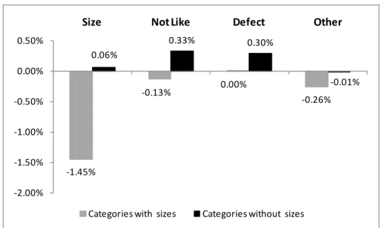
In Figures 1 and 2 we report the average difference between a customer’s first purchase in a category and their last purchase in a category according to whether: (a) the item is in the Childrens’ category or not and (b) whether the items in the category have sizes or not. The unit of observation is a customer in a category, and we use all of the observations for which the customer made at least two purchases in the category (so that we can calculate the change in the return rate). We report the difference in return rates for each of the four return reasons.
Figures 1 and 2 about here
There are several findings of interest. First, for categories without sizes there is essentially no change (0.06%) in the return rates due to size between a customer’s first and last category order. Further investigation confirms that the first and last return rates due to size are essentially zero in these categories. This is precisely what we would expect and offers reassurance that the return rate for sizes does not include returns for other reasons. Second, for those categories with sizes we see a large reduction (-1.45%) in the return rate due to sizes between customers first and last orders. This is consistent with our interpretation that customers learn about sizes as they place more orders in these categories. Third, the reduction in the return rate due to sizes is considerably smaller for Childrens’ categories than for other categories (-0.88% versus -1.50%). This is consistent with customers learning less about sizes from past purchases in Childrens’ categories than in other categories.
The change in return rates for the other three return reasons are also interesting. For these other return reasons the differences between categories with and without product sizes, and between
Childrens’ and other categories are much smaller than we observe for returns due to size. However, the sample sizes are very large and so even these smaller differences are statistically significant. It appears that when a customer returns an item because of poor fit this is generally categorized accurately as a size-related return. However, the larger reduction in returns on categories with sizes for these other three return reasons could indicate that some of the size returns spillover to these other return reasons. These attributions are not necessarily errors. Notice that a customer who finds that an item does not fit could quite reasonably indicate that they do not like the item, or interpret the poor fit as a defect. Any measurement errors that result from these spillovers will hinder (not help) validation of our prediction that the response to the competitive advertising event is associated with the change in the size return rate.
Return rates due to defects and because customers do not like the items exhibit a slight increase in categories without sizes. One possible explanation is that Retail World has a generous returns policy
16 | P a g e and the increase in return rates in these two categories may reflect customers learning about this policy. If this explanation is correct then, in the absence of learning about sizes, we might expect return rates in every product category to be higher for the last purchase than for a customer’s first purchase.
The Change in Return Rates and the Response to the Competitors’ Advertising
Our analysis again focuses on the 35 largest product categories. However, in this analysis we add an additional refinement to our definition of a category. Preliminary investigation revealed that for some apparel items Retail World uses different “size types”’ within a category. For example, women’s pants come in 3 different size types:
• {S, M, L XL, XXL …} • {1, 2, 3, 4, 6, 8, …}
• 23”, 24”, 25”, 26”, 28”, 30”, 32”, 34”
We would expect that learning would only occur within one of these narrow product categories. For example, learning about {S, M, L XL, XXL …} sizes may not help customers learn about {1, 2, 4, 6, 8, …} sizes. For this reason we use our separate sample of 3.6 million customers to identify the most common size type within each category and in our Size Learning analysis restrict attention to purchases and returns within this size type.14
To construct a category-level measure of the amount of learning about sizes in each category we calculated the difference in the return rate between a customer’s first and last purchase in each category and then averaged across customers. Because there is heterogeneity in the number of orders that customers place in different categories, we used two different approaches. In the first approach we averaged all customers who placed at least two orders in the category, while in the second approach we restricted attention to customers who had made exactly three orders in the category. The second approach was suggested by a reviewer and controls for heterogeneity in the frequency of orders across categories. As we would expect the two measures are highly correlated; the pair-wise correlation between them across the 35 categories is 0.97.
In Table 6 we report the pair-wise correlation between these two measures and the response to the competitors’ advertising event measured by the number of units purchased during the twenty month Measurement Period. We report the pair-wise correlations separately for all four return reasons. The key finding is that the faster the reduction in the return rate due to sizes between a customers’ first and last orders, the larger the response to the competitive advertising. This is consistent with the
explanation that customers returned to purchase from Retail World because they had learned about product sizes from previous purchases. The rank-order correlation between the change in returns due to size and the response to the competitive advertising is even larger (0.50), indicating that the
relationship cannot be attributed to mere outliers.
Table 6 and Figure 3 about here
14 The demand depletion interpretation that motivated our analysis of the recency of customer’s prior category purchases is not sensitive to these size types. For example, purchasing a size L pair of pants may deplete demand for size 10 pants as well as size L pants.
17 | P a g e In Figure 3 we provide a scatter plot of the response to the competitors’ advertising (in each category) and the change in return rates due to size. The relationship is clearly observable in this figure. The figure highlights why we observe a null overall effect; the impact of the competitive advertising is positive in some categories and negative in others. The figure also illustrates the magnitude of the interaction effect. In particular, if we group the 35 categories into quintiles (of 7 categories each) according to the change in returns due to size, the mean response to the competitors’ advertising in each quintile is monotonically decreasing. The first quintile (the leftmost portion of Figure 3) has the largest decrease in returns due to size and a mean response of 0.87%. In contrast, this effect declines to -1.8% and -3.1% in quintiles 4 and 5 (the rightmost portions) which have the smallest decrease in returns due to size. Importantly, this segmentation of the data clearly highlights the competing positive and negative effects of competitive advertising. We do observe negative advertising effects, but these are limited to categories with low consumer loyalty (the reduction in returns is smallest). Positive spillovers exist, but are limited to categories with high consumer loyalty (the reduction in returns is largest). While learning about sizes appears to play an important role in explaining the variation in the response to the competitive advertising, learning about the other return reasons is apparently less important. We do see a negative correlation between the other three return reasons and the response to the
competitive advertising. However, none of these correlations are statistically significant.
Number of Prior Purchases
Our interpretation of the change in returns measure suggests that customers who have made more prior purchases in the category should have learned more about products sizes. However, we have not directly tested how the response to the competitive mailings varies according to the number of prior purchases a customer has made in a category. Doing so requires that we overcome an important confound. A customer who has made more prior purchases from Retail World in a category may be more loyal to Retail World for reasons other than their knowledge of sizes (to aid exposition we will label this “generic loyalty”). An increase in purchases from Retail World as a result of receiving competitors’ advertising may just reflect this generic loyalty.
To demonstrate that the relationship between prior purchases and the response to the competitive advertising (if any) is due to learning about sizes rather than just generic loyalty, we will again rely on a comparison across categories. In particular, the generic loyalty explanation operates for every category, while we only expect prior purchases to contribute to learning about sizes in some categories. If we can show that the relationship between prior purchases and the response to the competitor’s advertising is stronger in categories in which there is more learning about product sizes, we can claim that the relationship is attributable to customer learning rather than other sources of loyalty.
We begin by constructing a measure of the rate at which customers learn about product sizes in each category. In particular, for each category we estimate how the change in returns (between the first and last order) varies according to the total number of orders a customer has made in the category. The slope of this relationship provides a measure of how quickly customers learn from previous orders. In categories in which customers learn more about the firm’s products we would expect this slope to be more negative, so that greater learning leads to a faster reduction in returns. For ease of exposition we
18 | P a g e label this slope the “Return Trend”.15
We then construct a measure of how much we expect each customer to have learned about sizes in each category by multiplying this measure of the rate of learning with the number of orders that customers have placed in each category:
A large positive Return Trend indicates that customers quickly increase their rate of returns (across orders), while a large negative trend indicates that the rate of returns quickly decreases.
Size Learningi,c = Return Trendc * Prior Category Ordersi,c
We add this variable to the QML Poisson customer x category-level model used to estimate the recency interactions in the previous section. In particular, we include both Size Learning as a main effect, and an interaction between Size Learning and the Treatment variable. It is the coefficient for this Treatment interaction that is the coefficient of interest. We caution that the interpretation requires care because this is a 3-way interaction between the Return Trend, the number of Prior Category Orders, and the
Treatment variable. The coefficient measures how an increase in the number of prior customer orders
affects the response to competitors’ advertising in categories in which there is a lot of learning about product sizes compared to categories without a lot of learning about product sizes.
Recall from our earlier discussion that Category Recency is not well-defined if a customer does not have a prior purchase in a category. It was for this reason that when we investigated the Treatment *
Category Recency interaction in the previous section we omitted these observations. In order to retain Category Recency as a control in our Size Learning model we use two different approaches. First, as in
Section 3 we estimate the model when omitting observations for customers with no prior purchases in a category (Model 1). In the second approach we include these observations and constructed a binary flag identifying customers with no prior purchases in a category.16 We include this binary flag as both a main effect and interacted with the Treatment variable (Model 2). This second approach recognizes that while these observations do not contribute to our understanding of the Category Recency interaction, they may provide insight in this model. In particular, customers with no prior category purchases cannot have learned any size information from past purchases. Our interpretation that learning about sizes contributes to customer loyalty suggests that the competitors’ advertising should have a smaller effect on purchases from Retail World for these observations.
The findings are reported in Table 7 (we again cluster the standard errors by category). In both models the coefficient for the interaction between Treatment and Size Learning is negative and highly
significant. This indicates that the response to the competitive advertising was higher among customers who had more prior experience in categories where the Return Trend is more negative. It is consistent
15 In each category we use OLS to estimate the Return Trend using the separate sample of 3.6 million customers. We use all customers who placed at least two orders in the category. The average sample size for these estimates is approximately 143,000, with a minimum of 10,000 observations in any category.
16 Notice that in Model 1 the sample size is smaller than the sample size for the models reported in Table 4. This reflects the narrower definitions of a category to focus on a single size type.
19 | P a g e with the interpretation that prior purchases lead to more loyalty in categories in which customers learn more quickly about product sizes.
Table 7 about here
We also observe a negative interaction between the Treatment variable and No Prior Category Purchase. This is consistent with our prediction that these customers would have a less favorable response to the competitive advertising. Notice that for these customers both Category Recency and Prior Category
Units equal zero, and so the estimated net impact of the Treatment on category sales for these
customers is -6.62% (adjusting the 3.28% main Treatment coefficient with just the -9.90% No Prior
Category Purchase interaction coefficient). This result highlights the mix of positive and negative
treatment effects. We observe a positive main effect from advertising but a negative effect among customers who have no history in a category.
5. Conclusions
Standard models of competition predict that firms will sell less when competitors target their customers with advertising. We have presented findings that contrast with this prediction and demonstrated that advertising can lead to positive spillovers for other firms even in a competitive market. We investigate how these positive spillovers vary across product categories. The findings reveal that the product categories with the largest spillovers are the categories in which customers appear to learn about product attributes from prior purchases. Detailed data on the reasons that customers return items allowed us to investigate what customers are learning. We show that the rate that customers learn about size information is closely related to the response to the competitive advertising.
We also investigated how the response to the competitive advertising varied according to how many times customers had previously purchased in a category. We find that customers who have made more prior purchases were more likely to respond to the competitors’ advertising by purchasing at Retail World. However, this only holds in product categories in which there is evidence that customers learn about product sizes from prior purchases. This distinction is important; it suggests that the relationship between past purchasing and the positive spillovers can be attributed to learning about product sizes, rather than other generic sources of customer loyalty.
Our findings provide unique measures of the impact of advertising in a competitive market, and we believe that the results have the potential to change our understanding of competition in mature markets. First, we show that advertising by a competitor may increase another firm’s sales. This result can be compared with previous studies of competitive advertising, which have generally focused on negative spillovers. For example extensive research in the tobacco industry has studied whether tobacco advertising leads to brand switching or an increase in primary demand: does Marlboro advertising lift Marlboro sales by increasing smoking, or by switching smokers from Rothmans to Marlboro? Few empirical studies anticipate the possibility of positive spillovers from competitors’ advertising, such as a positive impact of Marlboro advertising on sales of Rothmans.