Publisher’s version / Version de l'éditeur:
American Journal of Nano Research and Applications, 5, 1, pp. 1-6, 2017-04-17
READ THESE TERMS AND CONDITIONS CAREFULLY BEFORE USING THIS WEBSITE. https://nrc-publications.canada.ca/eng/copyright
Vous avez des questions? Nous pouvons vous aider. Pour communiquer directement avec un auteur, consultez la
première page de la revue dans laquelle son article a été publié afin de trouver ses coordonnées. Si vous n’arrivez pas à les repérer, communiquez avec nous à [email protected].
Questions? Contact the NRC Publications Archive team at
[email protected]. If you wish to email the authors directly, please see the first page of the publication for their contact information.
NRC Publications Archive
Archives des publications du CNRC
This publication could be one of several versions: author’s original, accepted manuscript or the publisher’s version. / La version de cette publication peut être l’une des suivantes : la version prépublication de l’auteur, la version acceptée du manuscrit ou la version de l’éditeur.
For the publisher’s version, please access the DOI link below./ Pour consulter la version de l’éditeur, utilisez le lien DOI ci-dessous.
https://doi.org/10.11648/j.nano.20170501.11
Access and use of this website and the material on it are subject to the Terms and Conditions set forth at
The linewidth broadening factor: a length-scale-dependent analytical
approach
Benhsaien, Abdessamad; Lu, Zhenguo; Hinzer, Karin; Hall, Trevor James
https://publications-cnrc.canada.ca/fra/droits
L’accès à ce site Web et l’utilisation de son contenu sont assujettis aux conditions présentées dans le site LISEZ CES CONDITIONS ATTENTIVEMENT AVANT D’UTILISER CE SITE WEB.
NRC Publications Record / Notice d'Archives des publications de CNRC:
https://nrc-publications.canada.ca/eng/view/object/?id=80ed0a00-3c4e-4b50-ba64-abbeff96a538 https://publications-cnrc.canada.ca/fra/voir/objet/?id=80ed0a00-3c4e-4b50-ba64-abbeff96a538http://www.sciencepublishinggroup.com/j/nano doi: 10.11648/j.nano.20170501.11
The Linewidth Broadening Factor: A
Length-Scale-Dependent Analytical Approach
Abdessamad Benhsaien
1, 2, 3, Zhenguo Lu
2, 3, Karin Hinzer
3, Trevor James Hall
31
Department of Mathematics, CÉGEP de l’Outaouais, Gatineau, Canada
2
Institute for Microstructural Sciences, National Research Council, Ottawa, Canada
3
Centrre for Research in Photonics, University of Ottawa, Ottawa, Canada
Email address:
[email protected] (A. Benhsaien)
To cite this article:
Abdessamad Benhsaien, Zhenguo Lu, Karin Hinzer, Trevor James Hall. The Linewidth Broadening Factor: A Length-Scale-Dependent Analytical Approach. American Journal of Nano Research and Applications. Vol. 5, No. 1, 2017, pp. 1-6. doi: 10.11648/j.nano.20170501.11
Received: February 28, 2017; Accepted: March 30, 2017; Published: April 17, 2017
Abstract:
A first-order frequency-dependent formula of the linewidth broadening factor (α–factor) is derived in terms of scattering rates whilst, a mesoscopic disk approach is used in order to accompany the dimension effect to the spontaneous emission lifetime (inverse of scattering rate). An excitonic correction to the relaxation properties is shown to occur provided the binding energy of the electron and hole is comparable to their eigenenergy-separation. The ensuing analysis is independent of the selected III-V material system and resides upon three simplifying assumptions which allow for analytical formulae to be derived.Keywords:
α–Factor, Linewidth, Enhancement, Scattering, Spontaneous Emission, Exciton, Mesoscopic, Quantum Dot1. Introduction
Semiconductor lasers host the dual quantized behavior akin to the light-matter interaction. Whereas, the micro-width of the embedded heterostructure waveguide cuts off high order photon modes, the nano-scale thinning along the vertical growth direction (such as in nano-structures) results in a discrete phase space of carriers. Given the recent advances in etching, patterning and growth methods, self-assembled quantum dot (SAQD) lasers are expected to have a considerably improved dynamic performance. Theoretically, a single quantum dot boasts a delta-like spectrum owing to its highly localized carriers. Yet, a single quantum dot may not display a nil α–factor around the material gain peak (homogeneous broadening) due to carrier scattering and other adverse broadening phenomena. The spectra of SAQDs get further broadened as a result of the spatial fluctuation in the resonance energy (inhomogeneous broadening). In the sequel, the α–factor dependence on the dimensionality is rigorously shown to be twofold, namely:
a) An explicit weak dependence emanating from the asymmetry of the active medium;
b) An implicit strong dependence emanating from the area/volume subject to the confining potential.
2. A Survey of the Measurment
Techniques
The calculation of the α–factor is at best a very subjective effort. The latter trait reflects the complex interplay of various coupled physical phenomena. It is a daunting task to isolate, let alone to assess, the effects of the major contributing phenomena while alienating those deemed to play a minor role. Moreover, the existing measurement techniques bear blatant discrepancies which are far from being reconcilable. To date, there has been remarkably no comparative study of the commonly used methods to measure the α–factor. Lately, the known measurement techniques have been applied to quantum dot media. Unlike numerical models predicting near zero α–factor, the experimental methods report a very wide range of values extending over the interval [0 a. u.; 60 a. u.]. Following are highlights of several experimental methods encountered in the literature:
a) The Hakki–Paoli method [1] directly measures the refractive index change - by detecting the frequency shift of longitudinal Fabry–Perot mode resonances - and the differential gain as the carrier density is varied by
2 Abdessamad Benhsaien et al.: The Linewidth Broadening Factor: A Length-Scale-Dependent Analytical Approach
slightly changing the current in a subthreshold regime. b) The Linewidth method measures the spectrum linewidth
and fits the results to known parameters, so that the α– factor can be extracted by applying Henry formula (equation (26) [2]).
c) The Modified Linewidth method measures the linewidth in terms of the emitted power in the threshold region, and the ratio of the slope of the linewidth vs. inverse power curve gives directly the α-factor [3].
d) The FM/AM method [4] relies on high–frequency current modulation which generates both amplitude (AM) and optical frequency (FM) modulation. The ratio of the FM to AM gives a direct measurement of the α– factor.
e) The Fiber Transfer Function method exploits the interaction between the chirp of a high–frequency modulated laser and the chromatic dispersion of an optical fiber, which produces a series of minima in the amplitude transfer function vs. modulation frequency. By fitting the measured transfer function, the α–factor can be retrieved [5].
f) The Optical Injection method, considers the light from a master laser being injected into a slave laser under test, to lock the slave optical frequency to that of the master. The locking region is characterized through the injected power level and frequency detuning, showing an asymmetry in frequency due to a non–zero α–factor [6, 7].
g) The Optical Feedback method is based on the self– mixing interferometry configuration and, according to the Lang–Kobayashi theory, the α–factor is determined from the measurement of specific parameters of the resulting interferometric waveform, without the need to directly measure the feedback strength [8].
Last, extreme caution must be exercised if interpreting the experimentally measured α–factor values or any other related parameters. The absence of a consensus regarding the α– factor formulae lends to speculations as to what parameter to draw a conclusion upon. For example, the α–factor can
equivocally be proportional to either the induced refractive index or effective refractive index change due to an elemental
variation of the injected carrier density into a microcavity. That alone may not ascertain the α–factor since the two interpreted figures are usually within two orders of magnitudes in an optical cavity.
3. A First-Order Approxiamtion to the
α–Factor
The α–factor is expressed in terms of the first-order susceptibility,
χ ν
( )1( )
= ℜe( )
χ
( )1 + ℑj m( )
χ
( )1 of the lasing medium. In particular, this allows scattering rates - responsible for broadening the spectrum line- and resonance parameters to be explicitly recast. Thus, it can be shown that:(
)
( )( )
( )( )
(
(
)
)
1 2 2 1 ; CV CV CV CV CV e N m N χ ν ν α ν ν ν χ ∂ ℜ − Γ ∂ Γ = = ∂ ℑ − − Γ ∂ (1)ν denotes here an oscillating frequency within a detuned
bandwidth centered at the resonant frequencyνCVof a
two-level system.ΓCVdenotes the transition rate (i.e. probability rate per unit time) of the carrier promoted from/to the valence state V to/from the conduction state C. 2ℏΓCV is the FWHM
of the broadening distribution as a result of the carrier-carrier scattering, carrier-phonon scattering and other dissipative scattering phenomena.
For simplicity, formula (1) assumes that:
A1: the transition energy ECVtr = EC−EV , the energy
separation of the valence state V and conduction state C, is independent of the carrier density;
A2: the difference in the occupation probabilities of the
states C and V fC− fV is independent of the carrier density.
A3: the energy separation between two consecutive
eigenstates is larger than the Boltzmann energy 25...30
B
k T ≈ meV.
The above three assumptions must not be confused with the fact that:
The eigenenergies E and EC V depend on the carrier density;
The (quasi-)Fermi-level and therefore the occupation probabilities fc and fv depend on the carrier density.
At resonance, in the presence of scattering, the α–factor is nil according to (1). Such is the ideal theoretical case. Note that the α–factor expression (1) applies to all spatial confinement dimensions alike.
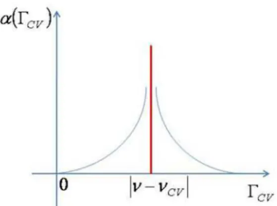
Away from resonance, and within a reasonable detuning bandwidth around νCV , two limiting cases need to be distinguished as depicted by the α–factor vs. scattering rate profile in figure 1:
The α–factor vanishes if the scattering rate approaches two unrealistic values, namely:
(
)
(
)
0 lim lim 0 CV CV CV CV α ν ν α ν ν + Γ →∞ Γ → ≠ = ≠ = .The α–factor shoots up asymptotically if the scattering rate approaches a physical singularity pointΓ = −CV
ν ν
CV ≠0.Note that the case 0 1
CV s
−
Γ ≈ corresponds to an infinite free carrier capture –into a bound state- lifetime making it physically unrealistic. Whereas, the case Γ → ∞CV
corresponds to extremely fast carrier dynamics given the short associated lifetime in this case. Either way, a low α– factor is constrained to scattering rates avoiding the latter extreme cases while being considerably far away from either side of the singularity point Γ = −CV ν νCV. Nonetheless, a
shorter scattering lifetime implies a faster consumption of the trapped carriers into the bound states (i.e. inside the active medium) causing the lasing threshold current to go up. In this manner, many carriers will not survive to relax farther into the deeper lying bound energy states (ground state for instance) and thus will not participate in lasing oscillations. Therefore, the quest for a low α–factor should be pre-constrained to scattering rates in the range
0< Γ << −CV
ν ν
CV in order to alleviate the carrier relaxation retardation.4. Spontaneous Emission Lifetime: Weak
Dimensionality Dependence
The recombination of an electron in the conduction band with a hole in the valence band is accompanied by the emission of a photon. The duality of the light-matter interaction grants that the time evolution, the spatial distribution and the spectrum of the spontaneous emission depend on the electromagnetic properties of the guiding medium. The latter attributes may be tailored within a resonating host medium such as a cavity. Thus, the quantum Hamiltonian of the optical field may be approximated by a combination of n independent harmonic oscillator Hamiltonians, each corresponding to a classical eigenmode of the optical field (i.e. photon) in the cavity with an oscillating frequencyνn.Many authors use the first quantized expression of the optical field since the concept of spontaneous emission comes out naturally in the treatment. The Fermi golden rule can be shown to give the spontaneous emission lifetime τsp (inverse of the transition probability
rate ΓCV) as:
(
)
2 1 , , 2 ; , sp CV q CV q TE TM σ σ τ− π κ δ ν ν σ = Γ =∑
− = (2)where the emitted photon has energy ℏνCVand momentum
q
ℏ . The polarization-dependent coupling of the electron to the optical mode is quantified through the constantκq,σ . Following Sugawara et. al. [9], an expression for the spontaneous emission lifetime is given by:
2 2 1 2 3 0 0 2 r CV , sp CV e n P TE TM m c σ ν τ σ ε − = = ℏ (3) Aside from being explicitly polarization dependent, formula (3) reveals also that the nanosecond-order
spontaneous emission lifetime is weakly dependent on the dimension of the spatial confinement. Such a dependence is borne by the matrix element PCVσ being inherently anisotropic for low dimensional media lacking geometrical symmetry [10]. No allusion in the literature is made to this fact; it is rather aberrantly assumed that the electron-hole spontaneous lifetime is dimension independent! (3) can thus furnish a preliminary means to investigate the weak dependence of the
α–factor on the dimension. As an illustration, the ratio of
spontaneous lifetime of a quantum-dot and a quantum-well is given by:
( )
( )( )
( )( )
( )( )
( )( )
( )( )
( ) 0 2 0 0 1 2 2 2 2 1 CV sp CV sp CV CV P A A P σ σ σ σ τ τ − − = = (4)where the dimension-dependent anisotropy factors ACV
σ have
been derived in [11].
Table 1. Dimension-dependent ratio of spontaneous lifetimes. C-HH TE C-LH ™ ( )( ) ( )( ) 0 1 2 1 − − sp sp τ τ 0.750 0.625
According to Henry’s formula [2], the linewidth ∆ν is proportional to 2
1+α . It follows from the results of table 1 that the emission line in quantum dots is at least 33% narrower than in the quantum well case. This implies that the
α–factor of the quantum dots enhances the spectra linewidth
by at least 15% for TE-polarized signals as it can be deduced from (4) that:
( )
( )( )
( ) ( ) ( ) 2 0 0 2 2 2 1 3 5 2 2 2 1 CV CV A A σ σ α α + = ≈ + (5)The linewidth enhancement of quantum dot media can attain 21% over that of quantum wells for TM-polarized fields according to (5).
5. Spontaneous Emission Lifetime:
Strong Dimensionality Dependence
Up until now, the interband electron-hole transitions have been considered irrespective of the energy binding the electron-hole pair. The electron-hole interaction in bulk media, through the Coulomb potential, will clearly be modified should both particles be confined along any spatial direction. Further localizing the electron and hole restricts the phase space of either particle causing its bound eigenenergies and momenta to be quantized accordingly. In parallel, the joint density of states undergoes a manifest change due to a strong dependence on the spatial confinement (i.e. material dimension). The latter dependence characterizes the optical susceptibility (absorption/gain) spectra.4 Abdessamad Benhsaien et al.: The Linewidth Broadening Factor: A Length-Scale-Dependent Analytical Approach
The optical susceptibility process involving the Coulomb interaction of the electron-hole pair is known as the excitonic susceptibility. A bulk exciton is composed of an electron in the conduction band and a hole in the valence band under the
Coulomb interaction. Excitons as bound states cannot exist
under the population inversion. In order for excitons to generate gain, the bound exciton emission energy (frequency) should be shifted from resonance through some mechanism such as scattering (refer to figure 1). The exciton selection rule ensures that a photon is emitted in the direction of the center-of-mass of the electron and hole two-particle system.
If the exciton interacts with the optical mode, the Fermi
golden rule can be shown again to give the exciton
spontaneous emission lifetime (inverse of the transition probability rateΓeg) as:
(
)
2 1 , , 2 ; , sp eg q g q TE TM σ σ τ− π κ δ ν ν σ = Γ =∑
− = (6)where νg denotes the exciton resonant frequency. The procedure to derive the exciton spontaneous lifetime is similar to that of the electron-hole pair [9]. The basic rules to derive the exciton lifetime in a quantum well are:
Momentum conservation: the selection rule of the in-plane wavevector is taken into account between the photon, q , ||
and the exciton center-of-mass motion, K(i.e. q||=K). Energy conservation: only excitons with a wavevector q ||
within a critical value qccan radiate spontaneously.
Due to the momentum conservation rule, the exciton spontaneous emission properties depend on the area/volume (i.e. strong dimension dependence) hosting the confining potential. This dependence is hidden in, the exciton to ground transition matrix element, Pegq,
σ
this time and can be expressed as in (7) for quantum wells:
(
) (
)
, || || , 0 q eg CV k P σ ≈Pσ Dϕ r = δ K −q (7) or, as in (8) in the case of quantum dots:( )
2 , 3 0; q eg CV ex P σ ≈Pσ∫
d Rψ R (8)Ris the exciton center-of-mass motion vector. The exciton wave function
ψ
ex(
r re; h)
=ϕ
(
re−rh)
×χ
( )
R can be separated into the ground state for the relative motion(
r re r)
ϕ
= − :( )
ex r ex ex e r λ ϕ π λ λ − = (9)and the wave function for the center-of-mass
( )
1 iKRR e
V
χ = (10)
This is in complete contrast to the electron-hole pair, whereby, the spontaneous emission lifetime is independent of the nanostructure dimension except in the transition matrix element (i.e. weak dependence) as highlighted in section 4.
Note that the wavevector selection rule for the center-of-mass motion is K=qand so the excitons emit photons along the direction ofK . This is a key concept to conceive the exciton-photon interaction and fast spontaneous emission in quantum wells.
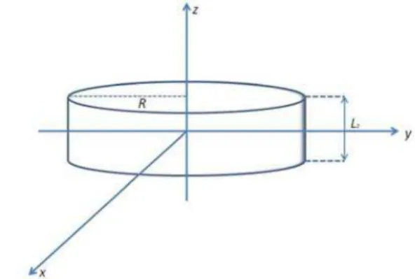
In order to witness the effect of the dimension on the spontaneous emission lifetime (and therefore the α–factor), the exciton is embedded within a mesoscopic disk as shown in figure 2. The disk has a radius R and its thickness Lz is at
most twice the Bohr radius of the exciton λex. The disk
consists of a direct bandgap semiconductor and it is assumed that both an electron and a hole are confined in the disk by the potential barriers of the surrounding regions.
Figure 2. Mesoscopic disk of radius R and thickness Lz.
When the radius R is much larger than the exciton wavelength, ( ex
r
R n
λ
>> ) the disk represents a quantum well with thickness Lz . The disk is mesoscopic when
2 eg ex r R n λ
λ < < where λeg is the exciton-to-ground transition
resonance. The disk is a quantum dot if 2
z
L
R≈ . This time, it
can be shown that [9]: ( )
( )
2 2 2 2 1 2 2 2 0 0 0 0 2 , c q q CV sp r eg e P qe dq m n TE TM σ β τ ϕ β πε ν σ − − = = ∫
ℏ (11)The picosecond-order spontaneous emission ratio depends on the areaπR2 =2πβ2
swept by the motion of the exciton center-of-mass. Formula (11) enables the analysis of the linewidth enhancement under different spatial confinement regimes through the mesoscopic radius
β
, namely:Microscopic region: R≤λex ⇔βqc <<1: The integral in equation (11) reduces to
0
c
q
qdq
(inverse) spontaneous lifetime is:
( )
( )( ) (
)
( )
( ) 2 2 2 2 0 0 1 2 2 0 0 0 2 2 2 CV c sp CV r eg e P q A m n σ σ β β τ ϕ πε ν − = ∝ ℏ (12) The factor β2in formula (12) represents the excitonic correction to formula (3) in the form of a mesoscopic enhancement to the linewidth.
Mesoscopic region 2 2 2 eg eg ex r c r ex R n q n λ λ λ β λ ≤ ≤ ⇔ ≤ ≤ :
The inverse spontaneous lifetime is given by:
( )( ) ( ) ( ) ( ) ( ) 2 2 2 2 2 2 012 1 2 2 2 2 2 0 0 1 1 0 2 c c q q CV sp r eg c c CV e e e P m n q q A β β σ σ τ ϕ πε ν − − − − − − − = ∝ ℏ (13) Macroscopic region: 2 2 2 eg eg c r ex R q n λ β λ λ ≥ ⇔ ≥ :
As
β
increases, formula (13) approaches that giving the inverse lifetime of a quantum well such that:( )
( ) ( ) ( ) ( ) ( ) 2 2 2 2 2 2 2 1 2 2 2 2 2 0 0 1 1 0 2 c c q q CV sp r eg c c CV e e e P m n q q A β β σ σ τ ϕ πε ν − − − − − = ∝ ℏ (14)In this manner, (13) connects continuously the microscopic and macroscopic limits of the scattering rates (inverse of the lifetime) via the mesoscopic regions. In order to observe the linewidth dimension dependence closely, we define the following ratio:
( )
( )( )
( ) ( )( )
( )( )
( ) ( )(
)
2 2 2 2 1 0 (2) (2) (0) 2 0 0 1 1 2 c q sp sp eg CV sp eg c sp CV weak strong e A q A β σ σ τ τ τ β τ − − − − Γ = = = × Γ (15)Figure 3. Linewidth mesoscopic enhancement under different spatial
confinement regimes.
Irrespective of the material system and its electronic structure, the ratio given by formula (15) allows a comparative analysis of the linewidth under different spatial confinements. In particular: ( )
( )
( )( )
( ) 2 0 (2) 0 0 lim c CV sp q sp CV A A σ β σ τ τ → =: Toward the quantum limit, the mesoscopic linewidth enhancement is at its maximum. Quantum dots of sizable dimension 0<<βqc≤1 , however, will observe a linewidth enhancement commensurate with the degree of confinement as can be seen from the microscopic region in figure 3. ( )
( )
( )( )
( ) 2 0 2 (2) 0 2 1 1 lim c CV sp q sp CV A e e A σ β σ τ τ → −= : In the mesoscopic region, the
stronger the confinement is, (i.e. the closer the normalized parameter βqc is to a unity), the better the linewidth
enhancement as can be seen observed from the mesoscopic region in figure 3. ( )0 (2) lim 0 c sp q sp β
τ
τ
→∞ = : As the disc radius exceeds2
eg r
n λ
, the exciton center-of-mass momentum K spreads outside the critical value of qcin the reciprocal space. Hence, the components
that never contribute to the spontaneous emissions increase. As expected, the larger the normalized parameter βqc is (i.e.
the weaker the spatial confinement), the less of an enhancement to the linewidth is observed as depicted by the macroscopic region in figure 3.
6. Spontaneous Emission Lifetime:
Temperature Dependence
Herein, the phonon-assisted interband transitions are carefully and purposefully alienated in favor of spontaneous emissions. Consequently, in view of assumption (A3), the
non-negligible spectrum broadening akin to the carrier-phonon scattering is neglected. A premise for this would be an astute epitaxial design whereby the lasing eigenstates are more than the Boltzmann energy apart. It is important to note
that assumption (A3), being completely physical, enables to
study the lasing characteristics irrespective of the controversial material parameters.
The exciton thermal distribution in the reciprocal Kspace induces an exciton emission lifetime dependence on the temperature as well. It remains to investigate closely how the change in dimensionality affects this temperature dependence. Resort is made to the mesoscopic disc approach so that progressive changes to the lifetime are made in terms of the spatial confinement.
Assuming that the thermal distribution in K||space is a Boltzmann distribution and averaging the lifetime over K||
space, the temperature dependence of the exciton lifetime in quantum wells is given as [10]:
1 1 1 ( ) (0 ) 1 c (0 ) T T c sp sp sp c T T K e K T T T τ− ≈τ− − − ≈τ− >> (16) where c c B c T q k
6 Abdessamad Benhsaien et al.: The Linewidth Broadening Factor: A Length-Scale-Dependent Analytical Approach
linearly with temperature in quantum wells.
In quantum disks, the temperature dependence of the exciton lifetime is given by [9]:
(
)
( )(
)
( ) 0 0 , 1 1 , , , exp ( ) (0 ) exp R r k n B k n sp sp R r kl nm B k l n m c E E k T T K E E k T τ− τ− ∆ + ∆ − ≈ ∆ + ∆ − ∑
∑
(17) where 00 R R R kl kl E E E ∆ = − and 10 r r r nm nm E E E ∆ = − . Thedenominator in (17) represents all the carrier distribution and the numerator represents the carrier distribution to the optically active states. The exciton binding energy is
r R
B nm kl
E =E +E . The lifetime increases as the temperature increases contributing thus to further thermal broadening of the line. By virtue of the result shown elsewhere [12], the stronger the confinement, the larger the energy separation between the active discrete states, equation (17) reduces in the case of zero-dimensional two-level energy system to a constant value
τ
sp−1( )T ≈τ
sp−1(0 )K . In quantum dots satisfying assumption (A3), the spontaneous lifetime is kept almost constant up to room temperature. Indeed, quantum dots do offer an alternative to quantum wells with minimal thermal line broadening.7. Conclusion
The present analytical study confirms that quantum dots shall have a linewidth broadening factor up to two orders of magnitude smaller than that of quantum wells. In fact:
( )
( )
( )( )
2 2 ( 2 ) ( 0 ) ( 2 ) ( 0 ) ( 2 ) 1 2 ( 0 ) ( 0 ) 2 ( 2 ) 2 ( 0 ) ( 2 ) 10 10 eg eg eg eg eg eg eg eg eg eg ns ps ν ν τ α α ν ν τ − Γ − − Γ Γ × = × ≈ = ≅ = Γ − − Γ Γ (18)The linewidth mesoscopic enhancement of (18) is primarily attributed to an acceleration of the carrier relaxation mechanism subsequent to additional spatial confinement. The classical study of the relative motion of the electron and hole and the exciton center-of-mass motion reveal that the enhancement is furnished in the form of an excitonic correction to the spontaneous emission lifetime.
The linewidth two-order-enhancement (18) is a gauge of further spectral purity of which, the potential can be reaped by tailoring the exciton within an advanced cavity such as lateral-coupling distributed feedback (LC-DFB) lasers [13, 14, 15].
References
[1] I. D. Henning, J. V. Collins, “Measurements of the semiconductor laser linewidth broadening factor”, Electron. Lett., 19, pp. 927, 1983.
[2] C. H. Henry, “Theory of the linewidth of semiconductor lasers”, IEEE J. Quantum Electron., 18, pp. 259-264, 1982. [3] A. Villafranca, J. A. Lázaro, I. Salinas and I. Garcés
“Measurement of the Linewidth Enhancement Factor in DFB Lasers Using a High-Resolution Optical Spectrum Analyzer”
IEEE Photon. Technol. Lett., 17, 2268-2270, 2005.
[4] C. Harder, K. Vahala, A. Yariv, “Measurement of the linewidth enhancement factor of semiconductor lasers”, Appl. Phys. Lett., 42, pp. 328-330, 1983.
[5] F. Devaux, Y. Sorel, J. F. Kerdiles “Simple measurement of fiber dispersion and of chirp parameter of intensity modulated light emitter” J. Lightwave Technol., 11, 1993.
[6] Hui, R.; Mecozzi, A.; D'Ottavi, A.; Spano, P, “Novel measurement technique of _ factor in DFB semiconductor lasers by injection locking”, Electron. Lett., 26, pp. 997 - 998, 1990.
[7] Liu, G.; Jin, X.; Chuang, S. L., “Measurement of linewidth enhancement factor of semiconductor lasers using an injection-locking technique”, IEEE Photon. Technol. Lett., 13, pp. 430 - 432, 2001.
[8] Y. Yu, G. Giuliani, S. Donati, "Measurement of the Linewidth Enhancement Factor of Semiconductor Lasers Based on the Optical Feedback Self-Mixing Effect", IEEE Photon. Technol. Lett., 16, pp. 990-992, 2004.
[9] M. Sugawara, “Self-Assembled InGaAs/GaAs Quantum Dots”, Semiconductors and Semimetals, vol. 60, Academic Press, 1999, 0-12-752169-0.
[10] S. L. Chuang, “Physics of Optoelectronic Devices”, Wiley Series in Pure and Applied Optics, 1995, ISBN 0471109398. [11] A. Benhsaien, “Self-Assembled Quantum Dot Semiconductor
Nanostructures Modeling: Photonic Device Applications”, MASc thesis, 2006.
[12] A. Benhsaien, T. J. Hall, “Self-Assembled Quantum Dot Semiconductor Nanostructure Modeling”, IEEE Journal of Optical and Quantum Electronics, OQEL565R1, 2008. [13] K. Dridi, A. Benhsaien, J. Zhang, T. J. Hall, “Narrow
linewidth 1560 nm InGaAsP split-contact corrugated ridge waveguide DFB lasers’’, Optics Letters 39 (21) · October 2014.
[14] K. Dridi, A. Benhsaien, J. Zhang, K. Hinzer, T. J. Hall, “Narrow linewidth two-electrode 1560 nm laterally coupled distributed feedback lasers with third-order surface etched gratings’’, Optics Express 22(16) August 2014.
[15] K. Dridi, A. Benhsaien, J. Zhang, T. J. Hall, “Narrow Linewidth 1550 nm Corrugated Ridge Waveguide DFB Lasers’’, IEEE Photonics Technology Letters 26(12):1192-1195 June 2014.