Bridging the Li-Carter’s gap: a locally coherent mortality forecast
approach
Quentin Guibert∗1,2,5, Stéphane Loisel†1, Olivier Lopez‡3, and Pierrick Piette§1,4
1
Univ Lyon, Université Claude Bernard Lyon 1, Institut de Science Financière et d’Assurances (ISFA), Laboratoire SAF EA2429, F-69366, Lyon, France
2
Ceremade, UMR 7534, Université Paris-Dauphine, PSL Research University, 75016 Paris, France
3
Sorbonne Université, CNRS UMR 8001, Laboratoire de Probabilités Statistique et Modélisation, LPSM, 4 place Jussieu, F-75005 Paris, France.
4
Seyna, 58 rue de la Victoire, 75009 Paris, France
5
Prim’Act, 42 avenue de la Grande Armée, 75017 Paris, France
February 7, 2020
Abstract
Countries with common features in terms of social, economic and health systems generally have mortality trends which evolve in a similar manner. Drawing on this, many multi-population models are built on a coherence assumption which inhibits the divergence of mortality rates be-tween two populations, or more, on the long run. However, this assumption may prove to be too strong in a general context, especially when it is imposed to a large collection of countries. We also note that the coherence hypothesis significantly reduces the spectrum of achievable mortality dispersion forecasts for a collection of populations when comparing to the historical observations. This may distort the longevity risk assessment of an insurer. In this paper, we propose a new model to forecast multiple populations assuming that the long-run coherent prin-ciple is verified by subgroups of countries that we call the "locally coherence" property. Thus, our specification is built on a trade-off between the Lee-Carter’s diversification and Li-Lee’s concentration features and allows to fit the model to a large number of populations simultane-ously. A penalized vector autoregressive (VAR) model, based on the elastic-net regularization, is considered for modeling the dynamics of common trends between subgroups. Furthermore, we apply our methodology on 32 European populations mortality data and discuss the behavior of our model in terms of simulated mortality dispersion. Within the Solvency II directive, we quantify the impact on the longevity risk solvency capital requirement of an insurer for a sim-plified pension product. Finally, we extend our model by allowing populations to switch from one coherence group to another. We then analyze its incidence on longevity hedges basis risk assessment.
JEL Classification: C18, C32, C53, J11.
Keywords: Coherent mortality forecasting; Multi-population; Basis risk; Vector Autoregression; Elastic-Net. ∗ Email: [email protected]. † Email: [email protected]. ‡ Email: [email protected]. § Email: [email protected].
1
Introduction
Around the world, the life expectancy of many countries has significantly risen over the past decades. This general augmentation implicitly suggests that common drivers are shared between populations such as lifestyle factors, the level of socioeconomic inequalities or the quality of the health system. However, this improvement is not equally shared among all groups of populations, precisely because the driving features are heterogeneous at an individual level. The links and differences between groups are important to understand for demographic and actuarial studies, since they may cause is-sues in managing social security system, pension funds or in defining longevity risk hedging solution. This explains the growing interest in mortality forecasting of multiple populations, especially to
un-derstand the effect of sub-groups on an overall population (Danesi et al., 2015; Bergeron-Boucher
et al.,2018; Cairns et al., 2019) or to enhance the projections robustness for populations with not
well-known trends, see e.g. Li et al. (2018).
Since the introduction of the augmented common factor approach by Li and Lee (2005), many
multi-population models have been developed. Most of them are extensions of the Lee and Carter
(1992) model or the CDB models (Cairns et al., 2006), and rely on a so-called coherence principle,
see Villegas et al. (2017) for a review. This concept, introduced by Li and Lee (2005), consists in
imposing that the mortality rates of two populations (or more) do not diverge in the long run. In such a specification, common age and period effects are estimated for a group of mortality data, the population specific trend being therefore modeled via mean-reverting process. This principle
is also introduced in the so-called GRAVITY model (Dowd et al., 2011) or in the Common Age
Effect (CAE) model (Kleinow, 2015; Enchev et al., 2017). Although this assumption may be
relevant for close populations, Li et al. (2017) have pointed out that it is often only suitable for
specific populations and over limited time windows. Hence, this approach is more likely to become unsatisfactory when it is applied to a large collection of populations. Furthermore, by inhibiting the divergence between populations, an irrelevant use of the mortality convergence principle may thereby distort the projections spectrum of mortality dispersion among the populations. In that context, extending the current mortality forecasting models for a large number of populations is challenging as it involves to cluster together similar countries and separately forecasting those with
diverging mortality dynamics, as noted by Richman and Wuthrich (2018).
Motivated by the need of applying stochastic mortality models to a large collection of popu-lations, our aim in this paper is to find a trade-off between the full coherence principle between populations and the noncoherence situation where single stochastic mortality models are considered independently. These two situations can be considered as border cases of the inter-group depen-dence possibilities, and are both undesirable, in a general context, for life insurers which are assisted by stochastic mortality multi-population models in their longevity risk solvency capital assessment. Indeed, a fully coherent model can overestimate the capital requirement through the concentration between the populations it imposes, whereas the use of independent single-population models may induce an underestimation of this capital. Note also that an inappropriate use of coherent mortality model for populations with heterogeneous mortality profiles or vice-versa can significantly affect the
effectiveness of reinsurance management strategies, see e.g. Yang et al. (2019). Similar problem
appears also for the pricing and the hedging of longevity risk transfer solutions where an accurate risk assessment is required, especially for the corresponding basis risk.
To overcome this issue, Li et al. (2017) introduce the concept of semicoherence which contains
the mortality differentials into a tolerance corridor. In other words, the two population mortal-ity dynamics can diverge over certain periods of time, but not permanently. Their semicoherent mortality projection is based on a threshold vector autoregressive process, which can be seen as a
vector autoregressive (VAR) model characterized by a parameter set and autoregressive order which
change according to the time series regime. Zhou et al. (2019) recently improve this approach by
introducing a threshold vector error correction model and taking into account long-term equilib-rium between time series. However, these models are developed for only two populations and their VAR structure contained many parameters, which is a serious limitation in the large-scale mortality forecasting framework.
In this paper, we propose an alternative approach, named "local coherence", which allows us to model simultaneously a large collection of populations by assuming the mortality coherence principle is satisfied for several subgroups of populations. Although our approach is mainly based on existing models, such as the Lee-Carter or the Li-Lee models, it intends to gain in flexibility by offering a trade-off between diverging mortality forecasts, obtained with a single stochastic mortality model,
and fully coherence forecasts. In that way, our goal is similar to the Li et al. (2017) semicoherence
one, i.e. offering a compromise between the fully coherence and the independence situations, even if the approach differs. Notably, in our case the size of the populations collection can be large and the proposed model includes the two border cases.
Within a locally coherent group, the dynamics of the mortality is based on a Li and Lee (2005)
model. To capture both long-term relationships and short-term interactions between groups, a VAR process models the improvements in the common mortality trends of each group. A similar specification for a small group of populations is proposed by several authors in the literature, see
Zhou et al. (2014), Kleinow (2015), and Enchev et al. (2017) among others. However, a VAR
model may suffer of over-fitting issue when the size of the group increases, since historical series are relatively short and strongly correlated. For our large-scale general context, we then use a VAR-ENET approach. Based on an elastic-net regularization technique, this VAR estimation is relevant with high dimensional time series and offers good in-sample and out-of-sample performances in a
mortality forecasting framework (Guibert et al., 2019).
For illustrative purpose, we estimate our locally coherent model on a collection of 16 European countries, by distinguishing the gender. We propose two approaches to cluster these populations in coherent groups, regarding to the historical mortality rates data or expert judgments. Our results highlight a better control of the mortality rates dispersion forecasting among the populations. In addition, we show the importance of having an accurate level of variability when considering the solvency capital requirement of an European life insurer exposed to longevity risks from multiple populations.
Furthermore, we extend our model by allowing the populations to switch dynamically from one group of coherence to another. Thus, the coherence may be specified locally not only in the spatial dimension, i.e. according to the populations, but also in the temporal dimension. Such switches can be caused by changes in socio-economic features driving the mortality dynamics. We underpin the importance this extension by analyzing the impact of a specific switch on a Longevity Divergence Index Value, similar to the one that the Kortis bond is based on.
The remainder of this paper is organized as follows. In Section2, we recall the usual Lee-Carter
and Li-Lee models and show the mortality dispersion forecasting issue. Section 3 introduces our
locally coherent model and shows how it fills the gap between a fully coherent and an independent
situations. We also present the VAR-ENET estimation method retained in the paper. Section 4
presents two clustering approaches for identifying coherent groups: one based on expert judgments and a data-driven approach. The results obtained on the groups composed of 32 European pop-ulations is discussed, and we demonstrate the interest for the risk-based capital requirement of a
local coherence, and illustrates its impact on a basis risk assessment example. Finally, Section 6
concludes the paper and gives several improvements for future researches.
2
The mortality dispersion issue
2.1 Notation
As noted in the Section1, a large range of models have been developed for mortality modeling and
forecasting within the multi-population framework. In this paper, we do not limit our study to the specific two-population context: we consider a more general scope of a collection I of populations,
where its cardinal Iě 2 is potentially high. Furthermore, we note X and T the collections of integer
ages and calendar years respectively.
For pi, x, tq P I ˆ X ˆ T , we note Dpiqx,t the number of people in the i-th population who die in
year t and aged x at their last birthday. The so-called "exposure to risk", noted Ex,tpiq, represents
the amount of person years lived by people of population i aged rx, x ` 1q in year rt, t ` 1q. Thus,
the central death rate mpiqx,t is given by
mpiqx,t “ D
piq x,t
Ex,tpiq
. (2.1)
In the two populations framework, the coherence can be analyzed by focusing on the difference
of log–mortality rates at a specific age x, which we note δx,t “ ln mp1qx,t ´ ln m
p2q
x,t. The coherence
hypothesis specifies that for all xP X , the series pδx,tqt do not diverge. We extend this measure to
the general multiple populations case where I is potentially important. Thus, for an age and time
px, tq, and a collection I of populations, we define δI
x,t the dispersion of mortality rates
δIx,t“ d 1 I´ 1 ÿ iPI ´ ln mpiqx,t´ ln mx,t ¯2 , (2.2) where ln mx,t “ 1I ř iPI
ln mpiqx,t is the mean of log mortality rates over the collection I. In this
way, this measure allows us to evaluate the heterogeneity of the mortality levels among a set of populations. The specific case of a coherent multi-population model corresponds to a situation
where for all xP X the dispersion`δI
x,t
˘
tPT is controlled and can not diverge.
2.2 The Lee-Carter model
There is a broad variety of mortality models that have been introduced in the actuarial science and demography literature. In this paper, we choose to focus on the Lee-Carter model, which is one of the most used by practitioners. We first quickly recall the model using the previous notation
and adopting a multi-population point of view. Thus, Lee and Carter (1992) propose to model the
central death rates of the i-th populaton such as
ln mpiqx,t “ αpiqx ` βpiqx κ
piq t ` ǫ
piq
where αpiqx and βxpiqare age-specific effect parameters, κpiqt represent the temporal mortality dynamics,
and ǫpiqx,t are residual terms. For the sake of the uniqueness of the solution, the usual constraints are
imposed in the estimation process
ÿ
tPT
κpiqt “ 0 and ÿ
xPX
βxpiq“ 1. (2.4)
Thus, αpiqx are set to be the averages of log mortality central rates over the period T considered,
and the series of parameters βpiqx and κpiqt are estimated thanks to the application of the singular
value decomposition (SVD) method.
Furthermore, we model the dynamic of the time series κpiqt as a random walk with a drift cpiq
κpiqt “ cpiq` κpiqt´1` epiqt , (2.5)
where the innovations ´epiqt ¯
iPI is an I–dimensional Gaussian white noises with mean 0 and a
diagonal variance–covariance matrix Σ1.
The Lee-Carter (LC) being a single population mortality model, we note that no relationships between the different populations are taken into account. As a consequence, the derived mortality forecasts are independent and can diverge. It creates a potentially large diversification effect on the projection of the longevity risk within a stochastic multi-population framework.
2.3 The coherent Li-Lee model
As an alternative, Li and Lee (2005) extend the Lee-Carter model to the multi-population scope by
imposing a common trend BI
xKtI to the collection I of considered populations, i.e.
ln mpiqx,t “ αpiqx ` BI xK I t ` βxpiqκ piq t ` ǫ piq x,t. (2.6)
The coherence is then enforced by modeling the dynamic of time series κpiqt via a mean-reverting
process. We retain here a first order autoregressive (AR) model
κpiqt “ apiqκpiqt´1` rpiqt , (2.7)
where the innovations´rtpiq¯
iPIare an I–dimensional Gaussian white noises with mean 0 and a
diag-onal variance–covariance matrix Σ2. We denote mIx,t the mortality rates of the overall population,
i.e. the gathering of all populations from the collection I
mIx,t “ D I x,t Ex,tI , (2.8) where DI x,t“ ř iPI Dpiqx,t and EI x,t “ ř iPI
Epiqx,t. Thus, the fit of a Lee-Carter model on these series, under
the usual constraints ř
tPT
KtI “ 0 and ř
xPX
the single population context, the age–population specific series of parameters αpiqx are set to be the
averages of log-mortality central rates over the training period T . Finally, the population–specific
temporal dynamic factors βxpiqκpiqt are obtained thanks to the SVD method, with the constraints
ř
tPT
κpiqt “ 0 and ř
xPX
βxpiq“ 1, for each i P I.
Similarly to the Lee–Carter model, time series KI
t is modeled as a random walk with drift
KtI “ cI ` Kt´1I ` eIt, (2.9)
where eI
t is a Gaussian white noise with mean 0 and related variance σI2.
Thus defined, the Li–Lee (LL) extension enforces the specific mortality rates of the whole collec-tion I of populacollec-tions to follow the same trend and converge in the long-run. Even if the populacollec-tion–
specific temporal factors κpiqt allow a population to slightly derives from this trend for a short period
of time, the mean–reverting property brings it back to the common dynamic over the long run. From a longevity risk management point of view, it then implies a limited diversification among the population in a stochastic evaluation context.
2.4 Mortality dispersion on the HMD
Let us now focus on a group of 16 western European countries, namely: Austria (AUT), Bel-gium (BEL), Switzerland (CHE), West Germany (DEUW), Denmark (DNK), Spain (ESP), Finland (FIN), France (FRA), Ireland (IRL), Italy (ITA), Luxembourg (LUX), Netherlands (NLD), Nor-way (NOR), Portugal (PTR), Sweden (SWE) and Great Britain (GBR). Furthermore, we consider separately the male and female populations for each country. Thus, our collection I of interest is
composed of I “ 32 populations, each one of them being defined by a couple pcountry, sexq. The
data is extracted from the Human Mortality Database (HMD, 2019). For the age–period training
set, we retain Xˆ T “ t45, . . . , 90u ˆ t1960, . . . , 2014u, and we fit single LC models as well as a LL
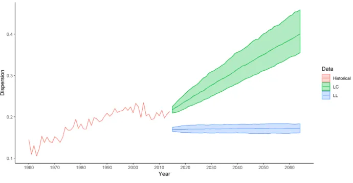
model, as described in Sections2.2 and2.3. The Figure 1 represents the dispersion δI
85,t estimated
on the historical data and on the projections over 50 years obtained with the both stochastic mor-tality models. For the latter, we plot the median together with the 95% prediction intervals derived from 500 Monte-Carlo simulations.
First, let us remark that the dispersion measure at age 85 has nearly doubled between the 1960’s and the 2000’s, and seems more stable in recent years. As expected, the predicted dispersion is significantly different between the results from the LC and the LL models. In the first case, both the median and the width of the prediction intervals of the dispersion increase linearly with the projection horizon. In other words, the mortality rates at age 85 of the considered populations become more and more dissimilar in average, and this heterogeneity significantly varies from one stochastic scenario to another. On the contrary, the LL’s forecasts exhibit a strongly stable disper-sion: according to them, not only the median is constant over time, but also the confidence intervals are very narrow comparing to the historical data and their bandwidth does not augment with the projection horizon. In term of generated mortality scenarios, it implies that a considerable majority of them lead to very similar pattern of mortality rates, even in the long term.
Both the LC and LL models present drawbacks when analyzing the projected dispersion in a longevity risk management framework. By not imposing any relationships between the population mortality dynamics, the LC model artificially creates some diversification in term of longevity risk. Contrariwise, the LL model imposes a strong coherence hypothesis on all the populations, thus leaving no significant scope for even a limited deviation of the mortality between the populations:
Figure 1: Dispersion at age 85 in the western European populations: historical data and median projections by Lee-Carter and Li-Lee models with the corresponding 95% prediction intervals. it assumes a high concentration risk in the longevity evaluation. Intuitively, a longevity risk manager may want to consider some intermediate scenarios between the exaggerated LC’s diversification and LL’s over–concentration.
3
A locally coherent approach
To bridge the gap between the Lee–Carter’s diversification and the Li–Lee’s concentration, we propose a new model based on the idea that the populations are coherent by homogeneous groups, and not all together at the same time. In the populations space, it can be seen as a local version of the coherence property.
3.1 The model
Keeping the notation introduced before, we now denote J a partition of the populations collection
I in J distinct groups. Let φ : I Ñ J be the corresponding classification function that labels a
population to a specific group. We then propose the following model for each population iP I
ln mpiqx,t“ αpiqx ` BxφpiqK
φpiq t ` 1t#φpiqą1uβxpiqκ piq t ` ǫ piq x,t, (3.1)
where # : J Ñ◆ is the cardinal function of a group, and φ piq denotes the coherence group of the
population i.
Similarly to the LL model, for each group j P J , the local common trend factors Bxj and Ktj
are estimated by fitting a Lee–Carter model thanks to the SVD method on the group log mortality rates data
mjx,t “ D j x,t Ex,tj , (3.2) where Djx,t“ ř iPj Dpiqx,tand Ex,tj “ ř iPj
Ex,tpiq, with the usual uniqueness constraints. For each population
i, the series of age factors αpiqx are set to be the averages of log mortality rates over the estimation
period T . Finally, the population–specific mortality dynamic parameters βxpiq and κpiqt are again
estimated through SVD, if the considered population i is assumed to be coherent with at least one of the other population.
To impose the local coherence, we keep the AR(1) dynamic of Equation (2.7) for the population–
specific period factors, but here we do not impose the variance–covariance matrix Σ2 of the
inno-vations´rpiqt ¯
iPI to be diagonal anymore. This allows to capture short–term relationships between
the populations.
Likewise, we also generalize the temporal dynamics of the period group factors to capture possible relationships between the different clusters of populations. Following the underlying idea of
Kleinow (2015) and Zhou et al. (2014), we retain a vector autoregressive (VAR) model. For j P J ,
we note ∆Ktj “ Ktj´ K
j
t´1 the common mortality improvement of the cluster. Given a temporal
lag p, the dynamic of the VARppq is then given by
∆Kt“ C ` p ÿ k“1 Ak∆Kt´k ` Et, (3.3) where ∆Kt “ ´ ∆Ktj¯
jPJ is the vector of mortality improvements at a group level, Ak, k “
1, . . . , p, are Jˆ J-autoregressive matrices, C is a J–dimensional vector of drifts, and Et is a J–
dimensional Gaussian white noise with mean 0 and Σ1 the related covariance matrix. The matrices
Ak, k“ 1, . . . , p, capture the long–run relationships of mortality improvements between groups of
coherent populations, while the variance–covariance matrix Σ1estimates the short–term dependence
structure of innovation shocks.
3.2 Border cases
Before continuing to the practical application of the model and its assessment, we focus on two special border cases. Indeed, by choosing some particular clusters and setting specific parameters, we note that our model includes the original Lee–Carter and Li–Lee models. To recover the LC model, we need to impose the following specifications:
• All the coherence clusters contain only one population, i.e. @i P I, φ piq “ tiu. In other words
we do not impose any coherence between the populations of interest.
• The temporal lag p of the VAR dynamic is set to 0. This point can also be approximated by
applying a high λ in the elastic–net estimation process. The vector C in Equation (3.3) is
then equivalent to the concatenation of the population–specific drifts cpiqfrom Equation (2.5).
• A diagonal structure is enforced to the variance–covariance matrix Σ1, i.e. no short–term
Similarly, we can also retrieve the LL framework from our model by considering the following constraints.
• All the populations are grouping into a single cluster, i.e. @i P I, φ piq “ I, the coherence
property is imposed to the whole demographic set.
• The temporal lag p of the VAR dynamic is set to 0. In particular, we remark that it is a 1–dimensional VAR due to the partition specification.
• A diagonal structure is enforced to the variance–covariance matrix Σ2. Further more, Σ1
being a 1ˆ 1–matrix, we recover the σ2
I of the LL’s common temporal trend dynamic.
Hence, our model framework can be seen as a bridge between the Lee–Carter and the Li–Lee ones. Thereby, for the rest of this paper, we denote it by LC–LL.
3.3 VAR Elastic–Net
In a general context, one can consider a large number J of groups by assuming that the coherence hypothesis is too strong for the populations of interest, thereby increasing dramatically the number of parameters to be estimated in the VARppq. From a statistic point of view, it may lead to high–
dimensional problems with a limited number of observations. Following Guibert et al. (2019), we
apply the extension of the elastic-net regularization and variable selection method proposed by
Zou and Hastie (2005) for the high-dimensional estimation of our autoregressive matrices. This
technique is a combination of the LASSO L1-penalty, introduced by Tibshirani (1996), and the
ridge L2-penalty developed by Hoerl and Kennard (1970). Elastic-net has similar properties of
variable selection as the LASSO. Moreover, it provides a grouping effect: highly correlated variables tend to be selected or dropped together. LASSO and elastic-net have already been extended to
VAR model (Gefang, 2014; Basu et al., 2015), mostly with an economic application (see e.g. Song
and Bickel,2011; Furman,2014) and more recently for mortality modelling (Guibert et al., 2019).
Therefore, we estimate the VARppq model presented in Equation (3.3) with T observations of
the process ∆Kt for tP T “ ttmin, . . . , tmaxu by minimizing the criterion
LpC, A1, . . . , Apq “ 1 T ´ p tmax ÿ t“tmin`p }∆Kt´ C ´ p ÿ k“1 Ak∆Kt´k}2 2 ´ αλ p ÿ k“1 }Ak}1´p1 ´ αq λ 2 p ÿ k“1 }Ak}22, (3.4)
where} . }1 and } . }2 respectively denote the L1 and L2 norms, λą 0 determines the strength
of the penalization, and αP r0, 1s represents the mix between ridge pα “ 0q and LASSO pα “ 1q
penalties. In particular, when α is set such as some LASSO penalty is enforced, i.e. α ą 0, the
higher λ gets, the fewer number of variables is selected.
For sparsity purpose we impose a larger weight to the LASSO penalty by setting α to 0.9. The hyper-parameter λ is then estimated thanks to a 10-folds cross-validation method. To apply this
estimation process, we use the sparsevar R-package (Vazzoler et al., 2016), which is based on the
glmnetone (Friedman et al., 2010). Furthermore, we choose to retain a temporal lag p“ 4 in the
4
Numerical applications
In this section, we compare the forecasting results with different locally coherent specifications
for European populations introduced in Section 2.4. First, we investigate clustering strategies to
determine the coherence groups among the collection of populations. We retain two approaches: expert–based and data–driven. Second, we focus on the main mortality trends that can be derived from these approaches, and their related stochastic scenarios spectrum. Finally, we illustrate the effect of the grouping assumptions on the solvency capital required of a pension product.
4.1 Population clustering
At first glance, the clustering methods can roughly be split between those based on expert judgments and those more data–driven. In the following, we give one example of each for the collection of
western European countries studied in the Section2.4. Our aim here is rather to give an outlook
of some reasonable clustering alternatives than describing exhaustively a methodology for grouping populations. Indeed, such an analysis is a complex task and is out of the scope of this paper,
since it requires to examine not only mortality data (Hatzopoulos and Haberman, 2013) but also
economical, social and environmental criteria as well as the health system of each population.
4.1.1 Coherence by country
In our case, the set of countries we are focusing on tend to strengthen their gender policy in the future. Thus, in the long run, one can assume that within a single country both male and female populations would have similar lifestyle with access to the same level of education, wealthiness
and healthcare, leaving mostly only biological differences. Thereby, we define the partition JM F
such as it clusters the populations by countries. The number of groups J equals then to 16. The corresponding model is noted LC–LL(MF).
An interesting point of this approach is that the VAR model estimates a dependence structure between the countries, allowing a rather easy reading of the autoregressive matrices that represent
the underlying dynamics. Indeed, the common period factors´Ktj, jP JM F
¯
are equivalent to the ones obtained by fitting single population LC models on the overall country. We display the Granger
causality matrices in Figures 8ato 8d of theAppendix 2.
4.1.2 A data mining approach
The main idea of the coherence in the Li–Lee model is to impose a common trend `KI
t
˘
tPT in
the mortality dynamics of each population i. This is done by fitting a Lee–Carter on the overall
population of the retained collection I (see Section2.3). Hence, for a single population i, we consider
its time series´κpiqt ¯
tPT, derived from the LC fitting, as a signature of the mortality dynamics.
To determine the coherence groups, we then apply an unsupervised clustering method on these signatures. We choose the well-known hierarchical cluster analysis (HCA) method. In particular, we retain the Euclidean metric and Ward’s criterion as dissimilarity measure and linkage criterion
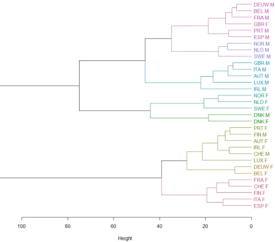
respectively. We display the corresponding dendrogram in Figure2.
We remark that, unlike the previous clustering, the populations are not gathered by country. It even seems to be the opposite: the gender indicator is one of the major splitting criteria. Yet, we
Figure 2: Dendrogram associated with the HCA applied on the LC’s κt, colored according to 8
final clusters. The acronyms for countries are defined in Section 2.4; F and M represent female
and male populations.
note one exception to this comment: the two Danish populations are clustered together, apart from other countries, suggesting that the Danish mortality dynamic exhibits some specific features when comparing to other western European countries.
For the following numerical applications, we choose to retain 8 different clusters, which are
emphasized in the Figure2 through the colors and recalled in the Table 1. We denote the LC–LL
mortality model based on this clustering by LC–LL(HCA8), and the corresponding partition by
JHCA8.
4.2 Dispersion forecasting
We now compare the models that we introduced, i.e. LC, LL, LC–LL(MF) and LC–LL(HCA8), int terms of dispersion. Rather than focusing on the main mortality trends that can be derived from these models, we are more interesting in the scope of this paper to the stochastic scenarios spectrum generated by these models.
Table 1: 8 groups of populations determined by HCA on the LC’s κt.
Group 1 Group 2 Group 3 Group 4 Group 5 Group 6 Group 7 Group 8
DEUW M NOR M GBR M NOR F DNK M PRT F DEUW F FRA F
BEL M NLD M ITA M NLD F DNK F FIN M BEL F CHE F
FRA M SWE M AUT M SWE F AUT F FIN F
GBR F LUX M IRL F ITA F
PRT M IRL M CHE M ESP F
ESP M LUX F
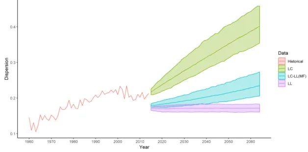
Following the Section 2.4, we display respectively in Figures 3 and 4 the projections obtained
from the LC–LL(MF) and LC–LL(HCA8) approaches, compared to the LC and LL model forecasts.
The red lines correspond to the historical dispersion δI
85,t for the 32 European populations of I at
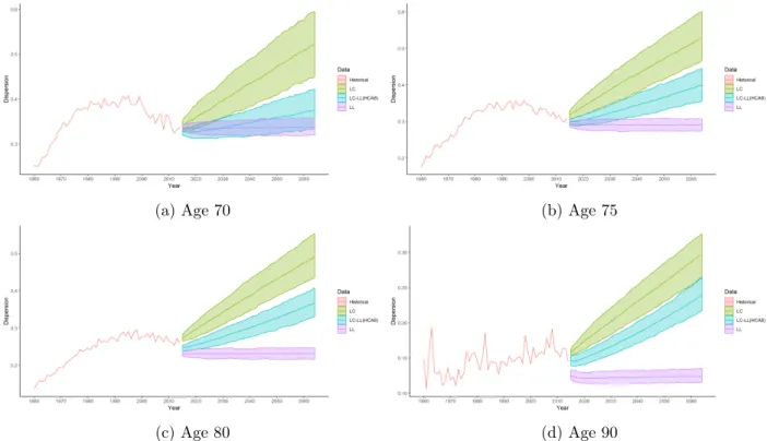
age 85. The same graphs are displayed inAppendix 1 for ages 70, 75, 80 and 90. As expected, the
dispersion predictions produced by the LC–LL models are contained between the LC and LL ones.
Figure 3: Dispersion at age 85 in the western European populations: historical data and median projections by LC, LL and LC–LL(MF) models with the corresponding confidence intervals at 5%
and 95%.
In the LC–LL(MF) case, we note that the dispersion level is comparable to the LL’s projection during the first years, however both the mean dispersion and the width of the confidence intervals are increasing with the projection horizon like in the LC model. This increase is yet significantly slower than the one obtained with the single population framework. While the latter causes a doubling of the dispersion within 50 years, the LC–LL(MF) leads to a dispersion spectrum relatively close to the historical observations of this measure since the 1990’s.
When focusing on the LC–LL(HCA8), we observe that the dispersion dynamic is similar to the LC: both of the models leads to a significant augmentation of the dispersion compared to the historical data. However, in the multi-population model, the increases of the main trend and confidence intervals are more limited. In term of longevity risk, it leads to a significant lower diversification level among the populations.
Figure 4: Dispersion at age 85 in the western European populations: historical data and median projections by LC, LL and LC–LL(HCA8) models with the corresponding confidence intervals at
5%and 95%.
4.3 Solvency Capital Requirement evaluation
Finally, we quantify the impact that the different models could have for a global (re)insurance company in terms of solvency capital requirement evaluation with respect to the longevity risk. To do so, we analyze a simplified situation where the liabilities are pensions to be paid between ages 60 to 90 for each of the 32 populations. Moreover, we focus only on the cohort aged 59 in 2014 and assume that at the valuation date, i.e. end of the year 2014, the number of pensioners is the same in every population. For the sake of simplicity, we retain an annual pension of 100 paid at the end of the year, and a constant discount rate of 1%.
Hence, to evaluate the corresponding provision the actuary needs to forecast the mortality
rates mpiq59`t, 2014`t for pi, tq P I ˆ t1, . . . , 32u. Following the Solvency II framework, the associated
longevity risk solvency capital requirement (SCR) is obtained by estimating the Value at Risk (VaR) at a 99.5% level of the best estimate provision. This is done by simulating 2,000 longevity scenarios
through the stochastic mortality models. We display in the Table2the results of this approach for
the LC, LL, LC–LL(MF) and LC–LL(HCA8) models.
Table 2: Best estimate provision and Solvency capital requirement estimates.
LC LL LC–LL(MF) LC–LL(HCA8)
Provisions (mean) 67,513 67,577 67,675 67,485
VaR 99.5 % 68,059 69,591 68,999 68,954
SCR (VaR - mean) 547 2,014 1,323 1,469
First, we remark that the choice of the model, among the collection we explore in this paper, does not impact much the provision. The absolute difference between the highest provision estimate and the lowest one is of 190, which represents less than 0.3% of the latter. On the contrary, the
range of SCR is significantly wider. As expected, the LC leads to the lowest value because the mortality scenarios are independent from one population to another, thus creating diversification. In comparison, the SCR estimated by the LL is nearly 3.7 times bigger. Indeed, in this case the mortality rate dynamics of all populations follow the same trend, thereby implying a concentration risk on this trend. Finally, between these two extreme modelings, our locally coherent approach
leads to intermediate levels of SCR. For the coherent groups determined in Section 4.1, we retrieve
approximately the average between the LC and the LL results.
5
Toward a dynamic local coherence
In our model introduced in Section3.1, we have supposed that the classification function φ : IÑ J
is constant through time. In other words, a population indefinitely belongs to the same group of coherence. However, in a more general longevity risk assessment framework, it could be interesting to study scenarios in which populations are allowed to switch from one coherence group to another. One of the motivations for such sensitivities is driven by the evaluation of basis risk in some longevity risk hedges. The aim of this section is to describe the stochastic forecasts of the mortality rates in a trend switching framework. Further, we highlight the effet of such switches on a Longevity Divergence Index Value (LDIV).
5.1 Trend switching model
Hereafter, the groups of local coherence j P J are rather to be considered as dominant mortality
trends which lead the mortality dynamics of their related specific populations. Thus, as long as a group of populations are lead by the same dominant trend, they are all coherent between them. On
the contrary to the model of Section3.1, we consider here that J is not necessarily a partition of the
retained collection of populations I anymore. However, it can always be viewed as a partition of a larger collection of populations Ω, which is not fully observed. Thus, depending of the time period,
some of the dominant trends j P J may not be linked to any retained population i P I. During
such periods, they can be viewed as dominant trends, exogenous from the observed collection of
populations. In the same way, we can assume that@j P J , #j ą 1, even if it implies assuming the
existence of populations in Ω which are not present in the retained collection of populations I.
Thus, forpi, x, tq P I ˆ X ˆ T , we propose the following dynamics for the central mortality rates
ln mpiqx,t“ αpiqx ` Bφ tpiq x K φtpiq t ` βxpiqκ piq t ` ad piq x,t` ǫ piq x,t, (5.1)
where function φt : I Ñ J return a set of classification functions, αpiqx are specific population
mortality levels,´Bxj, Ktj
¯
define the dominant mortality trends,´βpiqx , κpiqt
¯
represent specific
pop-ulation mortality dynamics, adpiqt,x are adjustment mortality levels. Considering the time series, we
keep the dynamics of the previous model, i.e. ∆Kt follows a VAR(p) model, see Equation (3.3),
and κpiqt are driven by AR(1) models.
The fact that the classification function φtis now dynamic, it may happen that the switch from
one dominant trend to another creates a significant leap in the mortality dynamics. Indeed, for
two different dominant trends pj1, j2q and a couple age–period px, tq, we do not impose the term
Bj2
dynamics. Thus, to avoid such jumps in the mortality level each time a population changes of dominant trend, we need to add adjustment mortality levels:
adpiqx,t “ t ÿ s“t0`1 Bφs´1piq x Ksφs´1piq´ Bφ spiq x Kφ spiq s , (5.2)
where t0is a time such as adpiqx,t0 “ 0 for all ages x P X . In a practical point of view, φt0piq defines
the initial dominant trend of the population i. Furthermore, we note that, in the non-switching
model case, we have@s P T , φs´1piq “ φspiq “ φ piq, so @t P T , adpiqx,t “ 0. Hence, we retrieve the
dynamics of the LC-LL with constant groups of coherence, see Equation (3.1).
5.2 European LDIV
As previously stated, this extension is motivated by the assessment of basis risk in longevity risk hedges. We choose to focus on one practical example: the Longevity Divergence Index Value (LDIV)
on which the Swiss Re Kortis bond is defined (Hunt and Blake,2015).
Issued in December 2010, the Kortis bond was designed to hedge the basis risk resulting from Swiss Re’s "partial natural hedge" in longevity risk. Indeed, the reinsurer was globally exposed to
• mortality risk on the US male population aged between 55 and 65, • longevity risk on the UK male population aged between 75 and 85.
Even though these two exposures create a natural longevity hedge, a significant basis risk remains between them two, especially if the mortality trends of the corresponding populations diverge. In our model, it would be implied by the fact that the two populations are not linked to the same dominant trend.
The payout of the Kortis bond is based on the level of the LDIV in 2016. To compute this value, we first need to observe the annualized mortality improvement of each population i
Improvementpiqn px, tq “ 1 ´ « mpiqx,t mpiqx,t´n ff 1 n , (5.3)
where n is the averaging period of the bond, equals to 8 years in the Kortis bond’s case. Then, an averaged improvement index is computed over the age classes exposed to the risk
Indexpt, iq “ 1 1` xpiq2 ´ xpiq1 xpiq2 ÿ x“xpiq1 Improvementpiqn px, tq , (5.4)
where for the Kortis bond the age classes are ´xpUKq1 , xpUKq2 ¯ “ p75, 85q and ´xpUSq1 , xpUSq2 ¯ “
p55, 65q. Finally, the LDIV at time t is obtained by
LDIVptq “ Index pt, i1q ´ Index pt, i2q , (5.5)
where in the Swiss Re casepi1, i2q “ pUK, USq and t “ 2016.
To illustrate the impact on the basis risk of a switch of dominant trend, we construct an European LDIV for:
• the Swiss female population, aged between 75 and 85, as the longevity risk exposure i1;
• the French female population, aged between 55 and 65, as the mortality risk exposure i2;
• a risk period n of 8 years, which ends at year t“ 2024.
Moreover, we suppose that at t0“ 2014, the mortality dynamics of the collection of populations
I follow the model of Section 4.1.2, i.e. the LC-LL(HCA8). Thus, the classification function φt0
can be described thanks to Table1. Finally, we suppose that at a time T ą t0, the French female
population switches from its original dominant trend to the dominant trend that the Belgian and German female populations are initially linked to. No further switch are considered. Hence, for
tą t0, we have φtpiq “ $ ’ & ’ % φt0piq if i‰ FRA F ,
φt0pFRA Fq if i “ FRA F and t ă T,
φt0pBEL Fq if i“ FRA F and t ě T.
(5.6)
Figure 5displays the sensibility of our European LDIV(2024) to the switching time T between
t0“ 2016 and 2024. To obtain the results, we simulate 10,000 stochastic mortality scenarios thanks
to our model for each switching time between 2016, i.e. the start of the risk period and 2024, i.e. the end of the risk period. We then retain the median scenario in term of LDIV(2024). As expected, the sooner the switch occurs, the more significant the Longevity Divergence Index Value is. In particular, we remark that the LDIV is 1.8 times higher when the switch happens in 2016 than in 2024. Indeed, the longer the French and Swiss female populations are linked to different dominant trends, i.e. the longer they are not coherent, the more they diverge.
Thus, our extended model allows the longevity risk manager to evaluate the impact of a wide spectrum of stochastic longevity scenarios on his portfolio and the potential hedges together with the corresponding basis risks. In a context where basis risk is one the main challenges that the
longevity risk transfer market is facing (Blake et al., 2019), our framework provides an innovative
point of view for its assessment.
6
Conclusions
In this paper we propose a new notion for multiple populations mortality forecasting that we have named local coherence. Indeed, we remark that full independence and "full" coherence approaches both suffer from drawbacks when considering the mortality projections of a large set of populations. To highlight this point, we compare the dispersion over 32 European populations of mortality rate
forecasts derived from Lee and Carter (1992) and Li and Lee (2005) models. In the first case,
the diversification in the stochastic scenarios is overestimated, whereas, in the second method, the concentration is exaggerated.
To overcome this issue, our locally coherent mortality model allows to forecast populations with homogeneous mortality profiles by coherence groups, where the long–term relationships between inter-group populations are only modeled through a VAR process without any coherence constraints. Thus, it offers a trade-off between the two border coherence cases, which are included in our model. The practitioners have then the possibility to easily simulate a larger spectrum of longevity scenarios to evaluate their risks compared to the usual models cited before.
Figure 5: Median European LDIV(2024) according to the switching time of the French female population.
To assess the behavior of our model, we have compared it with the Lee-Carter and Li-Lee’s ones over the set of European countries for some numerical applications. We notably show that the retained coherence hypothesis can have a major impact on the longevity risk solvency capital requirement for a global life insurance company within the Solvency II framework. Thereby, the large freedom of our model allows to evaluate more precisely this crucial risk measure.
Finally, we have extended the locality coherence property of our model to the temporal dimen-sion. By allowing populations to switch from one group of coherence to another, we expand the spectrum of possible stochastic mortality scenarios. This innovative methodology is particularly interesting in a longevity hedges’ basis risk assessment context. Thus, we propose a new framework that should be useful for the development of the longevity risk transfer market.
Our proposed method is a first step for modeling together both homogeneous and heterogeneous populations in terms of mortality profiles. It opens up some pathways for future research. We do not further investigate the difficult issue of how grouping a large set of populations. Our approach how-ever stresses the importance of developing techniques for identifying homogeneous/heterogeneous groups of population based not only on trend and volatility patterns in mortality dynamics, but also by considering economical, social and environmental criteria or the effectiveness of the health system. In addition, we also believe that groups of populations evolve dynamically. This means that some groups have a behavior which gradually converge to those of another groups, e.g. the
less developed countries would probably follow the trend of developed countries (Li et al.,2018), or
diverge from each other. Another potential improvement is thus to consider methods for detecting
References
Basu, S., Michailidis, G., and others (2015). Regularized estimation in sparse high-dimensional time
series models. The Annals of Statistics 43.4, pp. 1535–1567. doi: 10.1214/15-AOS1315.
Bergeron-Boucher, M.-P., Simonacci, V., Oeppen, J., and Gallo, M. (2018). Coherent Modeling and Forecasting of Mortality Patterns for Subpopulations Using Multiway Analysis of Compositions: An Application to Canadian Provinces and Territories. North American Actuarial Journal 22.1,
pp. 92–118. doi: 10.1080/10920277.2017.1377620.
Blake, D., Cairns, A. J. G., Dowd, K., and Kessler, A. R. (2019). Still living with mortality: the
longevity risk transfer market after one decade. British Actuarial Journal 24. doi: 10.1017/
S1357321718000314.
Cairns, A. J. G., Blake, D., and Dowd, K. (2006). A Two-Factor Model for Stochastic Mortality with Parameter Uncertainty: Theory and Calibration. Journal of Risk and Insurance 73.4, pp. 687–
718. doi:10.1111/j.1539-6975.2006.00195.x.
Cairns, A. J. G., Kallestrup-Lamb, M., Rosenskjold, C., Blake, D., and Dowd, K. (2019). Modelling Socio-Economic Differences in Mortality Using a New Affluence Index. ASTIN Bulletin: The
Journal of the IAA 49.3, pp. 555–590. doi:10.1017/asb.2019.14.
Danesi, I. L., Haberman, S., and Millossovich, P. (2015). Forecasting mortality in subpopulations us-ing Lee–Carter type models: A comparison. Insurance: Mathematics and Economics 62, pp. 151–
161. doi:10.1016/j.insmatheco.2015.03.010.
Dowd, K., Cairns, A. J. G., Blake, D., Coughlan, G. D., and Khalaf-Allah, M. (2011). A Gravity Model of Mortality Rates for Two Related Populations. North American Actuarial Journal 15.2,
pp. 334–356. doi: 10.1080/10920277.2011.10597624.
El Karoui, N., Loisel, S., and Salhi, Y. (2017). Minimax optimality in robust detection of a disorder time in doubly-stochastic Poisson processes. The Annals of Applied Probability 27.4, pp. 2515–
2538. doi:10.1214/16-AAP1266.
Enchev, V., Kleinow, T., and Cairns, A. J. G. (2017). Multi-population mortality models: fitting,
forecasting and comparisons. Scandinavian Actuarial Journal 2017.4, pp. 319–342. doi: 10 .
1080/03461238.2015.1133450.
Friedman, J., Hastie, T., and Tibshirani, R. (2010). Regularization Paths for Generalized Linear Models via Coordinate Descent. Journal of Statistical Software 33.1, pp. 1–22.
Furman, Y. (2014). VAR Estimation with the Adaptive Elastic Net. SSRN Scholarly Paper ID 2456510. Rochester, NY: Social Science Research Network.
Gefang, D. (2014). Bayesian doubly adaptive elastic-net Lasso for VAR shrinkage. International
Journal of Forecasting 30.1, pp. 1–11. doi: 10.1016/j.ijforecast.2013.04.004.
Guibert, Q., Lopez, O., and Piette, P. (2019). Forecasting mortality rate improvements with a
high-dimensional VAR. Insurance: Mathematics and Economics 88, pp. 255–272. doi: 10.1016/j.
insmatheco.2019.07.004.
Hatzopoulos, P. and Haberman, S. (2013). Common mortality modeling and coherent forecasts. An empirical analysis of worldwide mortality data. Insurance: Mathematics and Economics 52.2,
pp. 320–337. doi: 10.1016/j.insmatheco.2012.12.009.
HMD (2019). Human Mortality Database. University of California, Berkeley (USA), and Max Planck Institute for Demographic Research (Germany). Available at www.mortality.org (data down-loaded on 2019-07-08).
Hoerl, A. E. and Kennard, R. W. (1970). Ridge regression: Biased estimation for nonorthogonal
problems. Technometrics 12.1, pp. 55–67. doi: 10.1080/00401706.1970.10488634.
Hunt, A. and Blake, D. (2015). Modelling longevity bonds: Analysing the Swiss Re Kortis bond.
Longevity Risk and Capital Markets Solutions Conference 63, pp. 12–29. doi: 10 . 1016 / j . insmatheco.2015.03.017.
Kleinow, T. (2015). A common age effect model for the mortality of multiple populations. Insurance:
Mathematics and Economics. Special Issue: Longevity Nine - the Ninth International Longevity
Risk and Capital Markets Solutions Conference 63, pp. 147–152. doi: 10.1016/j.insmatheco.
2015.03.023.
Lee, R. D. and Carter, L. R. (1992). Modeling and Forecasting U. S. Mortality. Journal of the
American Statistical Association 87.419, pp. 659–671. doi:10.2307/2290201.
Li, H., Lu, Y., and Lyu, P. (2018). Coherent Mortality Forecasting for Less Developed Countries. SSRN Scholarly Paper ID 3209392. Rochester, NY: Social Science Research Network.
Li, J. S.-H., Chan, W.-S., and Zhou, R. (2017). Semicoherent Multipopulation Mortality Modeling: The Impact on Longevity Risk Securitization. Journal of Risk and Insurance 84.3, pp. 1025–
1065. doi:10.1111/jori.12135.
Li, N. and Lee, R. (2005). Coherent mortality forecasts for a group of populations: An extension of
the Lee-Carter method. Demography 42.3, pp. 575–594. doi: 10.1353/dem.2005.0021.
Richman, R. and Wuthrich, M. V. (2018). A Neural Network Extension of the Lee-Carter Model to Multiple Populations. SSRN Scholarly Paper ID 3270877. Rochester, NY: Social Science Research Network.
Song, S. and Bickel, P. J. (2011). Large vector auto regressions. arXiv preprint arXiv:1106.3915. University of California, Berkeley.
Tibshirani, R. (1996). Regression shrinkage and selection via the lasso. Journal of the Royal
Statis-tical Society. Series B (Methodological) 58.1, pp. 267–288. doi: 10.1111/j.2517-6161.1996. tb02080.x.
Vazzoler, S., Frattarolo, L., and Billio, M. (2016). sparsevar: A Package for Sparse VAR/VECM Estimation. R package version 0.0.10.
Villegas, A. M., Haberman, S., Kaishev, V. K., and Millossovich, P. (2017). A comparive study of two-population models for the assessment of basis risk in longevity hedges. ASTIN Bulletin: The
Journal of the IAA 47.3, pp. 631–679. doi:10.1017/asb.2017.18.
Yang, S. S., Yeh, Y.-Y., Yue, J. C., and Huang, H. C. (2019). Understanding Patterns of Mor-tality Homogeneity and Heterogeneity Across Countries and Their Role in Modeling Mortal-ity Dynamics and Hedging LongevMortal-ity Risk. North American Actuarial Journal, pp. 1–24. doi:
10.1080/10920277.2019.1662315.
Zhou, R., Wang, Y., Kaufhold, K., Li, J. S.-H., and Tan, K. S. (2014). Modeling Period Effects in Multi-Population Mortality Models: Applications to Solvency II. North American Actuarial
Journal 18.1, pp. 150–167. doi: 10.1080/10920277.2013.872553.
Zhou, R., Xing, G., and Ji, M. (2019). Changes of Relation in Multi-Population Mortality
Depen-dence: An Application of Threshold VECM. Risks 7.1, p. 14. doi: 10.3390/risks7010014.
Zou, H. and Hastie, T. (2005). Regularization and variable selection via the elastic net. Journal
of the Royal Statistical Society: Series B (Statistical Methodology) 67.2, pp. 301–320. doi: 10. 1111/j.1467-9868.2005.00503.x.
Appendix 1
Dispersion projections
(a) Age 70 (b) Age 75
(c) Age 80 (d) Age 90
Figure 6: Dispersion in the western European populations: historical data and median projections by LC, LL and LC–LL(MF) models with the corresponding confidence intervals at 5% and 95%.
Appendix 2
Granger matrices from the LC-LL(MF) model
The matrix A1 (Figure 8a) exhibits mostly negative coefficients, shaped into a diagonal structure.
We hereby capture the country–specific period effect. Indeed, when modeling the single population
LC’s κpiqt dynamics by an AR(1), we generally obtain negative autoregressive estimates. Displayed
in a matrix way for a multi-population point of view, it leads to a negative diagonal matrix. We also remark some vertical patterns within the Granger causality matrices. In term of mortality dynamics, this should be interpreted as a persistent effect of a single country to a group countries.
For example, in the autoregressive matrix A3 (Figure8c), we note the existence of a positive vertical
structure on the Swiss population. Hence, the Swiss mortality improvement seems to Granger cause the mortality improvement on 6 other countries, namely BEL, DEUW, GBR, IRL, NLD and PRT. A chock in the mortality rates in the Switzerland would then reverberate 3 years later in the 6 countries. In this way, the vertical structure can be seen as some kind of leader effect.
(a) Age 70 (b) Age 75
(c) Age 80 (d) Age 90
Figure 7: Dispersion in the western European populations: historical data and median projections by LC, LL and LC–LL(HCA8) models with the corresponding confidence intervals at 5% and 95%.
(a) A1 (b) A2
(c) A3 (d) A4
Figure 8: Estimated autoregressive matrices A1, . . . , A4 of the VAR-ENET from the LC–LL(MF)
model.