HAL Id: hal-01741613
https://hal.archives-ouvertes.fr/hal-01741613
Submitted on 23 Mar 2018
HAL is a multi-disciplinary open access
archive for the deposit and dissemination of
sci-entific research documents, whether they are
pub-lished or not. The documents may come from
teaching and research institutions in France or
L’archive ouverte pluridisciplinaire HAL, est
destinée au dépôt et à la diffusion de documents
scientifiques de niveau recherche, publiés ou non,
émanant des établissements d’enseignement et de
recherche français ou étrangers, des laboratoires
To cite this version:
Lynda Khiali, Dino Ienco, Maguelonne Teisseire. Object-oriented satellite image time series
anal-ysis using a graph-based representation.
Ecological Informatics, Elsevier, 2018, 43, pp.52-64.
�10.1016/j.ecoinf.2017.11.003�. �hal-01741613�
DOI: doi:10.1016/j.ecoinf.2017.11.003 Reference: ECOINF 822
To appear in: Ecological Informatics Received date: 12 July 2017
Revised date: 25 September 2017 Accepted date: 26 November 2017
Please cite this article as: Khiali, Lynda, Ienco, Dino, Teisseire, Maguelonne, Object-Oriented Satellite Image Time Series Analysis using a Graph-Based representation,
Eco-logical Informatics (2017), doi:10.1016/j.ecoinf.2017.11.003
This is a PDF file of an unedited manuscript that has been accepted for publication. As a service to our customers we are providing this early version of the manuscript. The manuscript will undergo copyediting, typesetting, and review of the resulting proof before it is published in its final form. Please note that during the production process errors may be discovered which could affect the content, and all legal disclaimers that apply to the journal pertain.
ACCEPTED MANUSCRIPT
Object-Oriented Satellite Image Time Series Analysis
using a Graph-Based representation
Lynda Khialia, Dino Iencoa,b, Maguelonne Teisseirea
aIrstea, UMR TETIS, Montpellier, France bLIRMM, Montpellier, France
Abstract
Nowadays, remote sensing technologies produce huge amounts of satellite im-ages that can be helpful to monitor geographical areas over time. A satellite image time series (SITS) usually contains spatio-temporal phenomena that are complex and difficult to understand. Conceiving new data mining tools for SITS analysis is challenging since we need to simultaneously manage the spa-tial and the temporal dimensions at the same time. In this work, we propose a new clustering framework specifically designed for SITS data. Our method firstly detects spatio-temporal entities, then it characterizes their evolutions by mean of a graph-based representation, and finally it produces clusters of spatio-temporal entities sharing similar temporal behaviors. Unlike previous approaches, which mainly work at pixel-level, our framework exploits a purely object-based representation to perform the clustering task. Object-based analy-sis involves a segmentation step where segments (objects) are extracted from an image and constitute the element of analysis. We experimentally validate our method on two real world SITS datasets by comparing it with standard tech-niques employed in remote sensing analysis. We also use a qualitative analysis to highlight the interpretability of the results obtained.
Keywords: Remote sensing data, satellite images time series, clustering, object based image analyses.
Email addresses: [email protected](Lynda Khiali), [email protected] (Dino Ienco), [email protected] (Maguelonne Teisseire)
ACCEPTED MANUSCRIPT
1. Introduction
Nowadays, modern satellite technologies are used to collect huge volume of Earth Observation data [1]. Such data constitute a rich source of information that is stored in remote sensing images archives. Such archives can be exploited to analyze areas that cannot be easily accessed by experts in order to then organize field campaigns in specific zones of interest.
Satellite images can be employed to remotely monitor artificial and natural phenomena such as urban areas expansion, changes in natural habitats, agri-cultural land use evolution, and climate change impacts [2, 3]. The analyses are performed by gathering time series of satellite images that consider the same spatial extent over different timestamps. While standard time series ap-proaches involve the study of independent phenomena that evolve over time [4], the analysis of time series of satellite images involves simultaneously considering the temporal dimension characterizing data evolution, and spatial interaction among the entities present in the data. This is why, due to the increasing vol-ume of remote sensing time series generated by modern satellites programs such as the Copernicus program 1, it is crucial to conceive and develop innovative
data mining tools to automatically browse and explore such data.
Another challenge related to remote sensing analysis is the granularity of the analysis we want to exploit in order to depict the underlying phenomena in the remote sensing time series [5]. Recently, [5] was one of the first studies to use object-based analysis instead of based one. While in the pixel-based analysis, the basic units evaluated are pixels, in object-pixel-based analysis, the images are first segmented and these segments (objects) become the basic units in any further analysis. Considering objects instead of pixels has two main advantages: i) objects represent a more coherent piece of information since they are simpler to interpret [6]; ii) objects facilitate data analysis scale-up since, for the same image, the number of objects is usually smaller than the number of
1
ACCEPTED MANUSCRIPT
pixels by several order of magnitude.
Object-based techniques are usually used to perform single (remote sensing) image analysis [5] while, for time series of satellite images, the pixel-based anal-ysis is still favoured since aligning pixels between two consecutive images (of the same resolution) is straightforward as you only have to superpose the images on the pixel grid.
Conversely, aligning objects coming from different images, of the same time series, can be problematic as there is no one to one correspondence.
To perform an object-oriented analysis of SITS data, we propose a novel 3-step methodology involving: i) the detection of spatio-temporal entities (i.e. agriculture plots, forests, meadows, rivers, lakes) from the time series ii) the description of each spatio-temporal entity by means of a graph-based represen-tation and iii) the clustering of the detected spatio-temporal entities to highlight common behaviors present in the study area. The last step of the methodology (the clustering approach) exploits a novel distance measure that simultaneously combines the content information coming from the spectral images and the graph topology supplied by the graph-based representation. The result is a set of clusters presenting spatio-temporal entities that present different evolution behaviors in the study area.
To automatically extract and describe spatio-temporal entities we leverage the method we previously proposed in [7]. For each detected entity, this method builds a graph-based description named evolution graph that summarizes the evolution of the spatio-temporal phenomenon.
We can summarize the contributions of our work as follows:
• We formalize a new framework to perform object-based clustering of Time Series of Satellite Images (SITS);
• We propose a new measure to evaluate distances between two evolution graphs such that any distance-based clustering algorithm can be used to obtain a partition of the evolution graphs ;
ACCEPTED MANUSCRIPT
study areas; we also compare our framework with state of the art methods used to clustering SITS data.
The remainder of this paper is organized as follows. Section 2 explores related works in the area of time series clustering with a major emphasis on satellite data. The proposed clustering framework is described in Section 3. Section 4 introduces the study areas involved in the experiments and it supplies details about data pre-processing. Quantitative and qualitative evaluations are made in Section 5. Finally, Section 6 provides the conclusions of our study.
2. Related work
In the data mining literature many approaches were proposed to cluster time series data [8, 4, 9, 10, 11]. Most of these approaches employ standard clustering algorithms and the novelty in the approach is linked to new ways of evaluating distance (similarity) between time series. One of the most well known measure, to deal with time series data, is Dynamic Time Warping (DTW) [12]. This kind of measure can be used to compute an optimal alignment between two given time series. It is usually employed for long time series that cannot be temporally aligned, and that could contain noise. DTW is generally costly to compute. In [8] the authors propose an approximate and less costly way to compute DTW. The results obtained using the new strategy are in line with the original measure.
In [4], the authors propose a new efficient complexity-invariant distance mea-sure to group together time series. The work underlines that the choice of a good similarity measure is generally more important than the choice of the clustering algorithm for a particular kind of time series data. The proposed measure seems suitable for time series clustering but it considers the objects to be clustered as independent from each other, unlike for remote sensing data where the instances to be clustered are spatially correlated to each other. A Minimum Description Length (MDL) method is proposed in [9]. The work de-fines a parameter-free strategy to cluster together time series considering the
ACCEPTED MANUSCRIPT
compression cost. Experiments show that this algorithm is effective on a wide variety of datasets.
Unlike standard time series analysis, in the remote sensing domain, spatial information plays a predominant role in the analysis of satellite images. For instance, in the works [13, 14, 15, 16] the decision tree approach is adapted to consider spatial regularization in order to reduce the salt-and-pepper noise that can be generated by a pixel-level analysis.
Considering the problem of clustering time series of satellite images, [10] proposes an approach that can deal with irregularly sampled time series. The clustering strategy uses DTW on multivariate time series at the pixel level. Each time series represents a pixel. The time series is built by concatenating the radiometric information of a pixel over the time. The approach has shown its robustness on noisy time series with different lengths.
In order to inject spatial information into the SITS clustering process, [11] in-troduces a methodology for spatio-temporal analysis that combines pixel and object-level information to produce the final clustering solution. Firstly, a seg-mentation is performed on each image of the time series, then the pixel time series is enriched with the object information in order to strengthen the con-nection between pixels belonging to the same segment. The final clustering is performed using the K-Means algorithm and the euclidean distance metric to evaluate proximity between time series. This method can be considered as a first step towards involving the spatial information supplied by object-based analysis. Nevertheless, the work still considers pixels as basic units to be pro-cessed. Another drawback of the approach is related to the time performance: considering pixels instead of objects can negatively influence the scalability of data mining algorithms since, for a given image, the number of objects is usually several order of magnitude smaller than the number of pixels.
ACCEPTED MANUSCRIPT
3. Methodology
In this section, we introduce the definition and the clustering framework we developed to mine time series of satellite images exploiting an object-based representation. To this purpose, we begin by introducing some definitions, then we supply a general overview of our proposal, and finally, we detail the different steps of our proposal.
3.1. Overview of the Methodology
Figure 1 summarizes the different parts of our framework.
Given a SITS data and their associated segmentation, we first select a set of objects that represent the spatial entities we want to monitor over time. We call this subset of objects Reference Objects. The set of Reference Objects (RefObjs) can contain objects coming from any timestamp (Fig. 1(Step1)). Next, for each Reference Object, we create an evolution graph considering all the segments, in all the timestamps, covered by its footprint. Each vertex of a graph corresponds to a segment. Two vertices are linked by an edge if they belong to two successive timestamps and the corresponding objects overlap each other. This allows us to link together objects that span over the same area over the time. The procedure is applied to each object of RefObjs and the result consists in a set of evolution graphs that summarize the different spatiotemporal phenomena existing in the study site (Fig. 1(Step2)). Once the set of evolution graphs is obtained, we propose a new way to compute distances between them in order to successively apply a clustering algorithm with the purpose of organizing and highlighting common patterns among data (Fig. 1(Step3)).
Figure 1: Overview of the different steps of the proposed framework to detect and cluster spatio-temporal entities.
ACCEPTED MANUSCRIPT
3.2. Preliminaries and Notations
For a given study area, we represent a remote sensing time series monitoring such area as an ordered set of images (I1, I2, ..., IT) where the index represents
the image timestamp. The ordered set of images is aligned and covers the same geographical area.
For an image It, we have a set of associated segments Ot= {oit} |Ot|
i=1 where t
is the image timestamp and i is the segment identifier related to the image It.
We wish to stress that the number of segments is not the same for all the images of the time series. We also denote with O the union of all segments belonging to any timestamp (O =Tt=1Ot). Associated to each segment, we can also retrieve
the set of pixels it contains (P ix(oi
t)) and the vector of (radiometric) information
(Inf o(oi
t)) describing its content. The feature vector associated to each segment
is obtained as the average of the radiometric values of its corresponding pixels. The pixel identifier always refers to the same zone. This means that, if two pixels at different timestamps have the same identifier, they correspond to the same geographical area as the different images are spatially aligned.
3.3. Entity Tracking by Graph-Based Representation
In [7], we proposed an automatic technique to track entity evolutions for a given time series of satellite images. The clustering framework leverages this approach to group together similar entities. The approach works at object level unlike to most of previous methods that, instead, consider pixels as the basic unit to study [10]. It consists of two main phases: i) Entity Detection and ii) Evolution Description.
The Entity Detection is aimed at selecting among the segments of all images, a set of reference objects (entities) to be monitored over the time series.
The reasoning behind this procedure is the follows: during the time series, each entity achieves its maximal signal. The maximal signal can be measured by means of its spatial extent. This means that, if we can select segments that cover big zones over the time series, while reducing their degree of overlapping,
ACCEPTED MANUSCRIPT
we can consider such segments as representative of the maximal spatial extents of the underlying entities.
We model this task as a covering set problem [17]: each segment represents a set of pixels and the resulting set needs to cover the study area as completely as possible while minimizing the overlapping among the different selected objects. Algorithm 1 reports the procedure to automatically detect the reference objects. Algorithm 1 EntityDetection(O, α) 1: Segments= O 2: Ref Obj=∅ 3: weight= 0 4: while|Segments| > 0 do 5: obj=−1 6: max weight=−1
7: for allo∈ Segments do
8: if P ix(o) P ix(Ref Obj) =∅ then
9: weight=|P ix(o)|
10: else
11: weight=|P ix(o)−P ix(Ref Obj)||P ix(o)|
12: end if
13: if weight < α then
14: Segments= Segments - o
15: else if weight > max weight then
16: max weight= weight
17: obj= o
18: end if
19: end for
20: ifobj#= −1 then
21: Ref Obj= Ref Obj∪ obj
22: end if
23: end while
24: returnRef Obj
Unlike with the original covering set problem [17], the strategy requires the complete set of segments O and the α threshold as parameters. This second parameter can be used to filter the least relevant segments (it ranges between 0 and 1). At each iteration, the algorithm selects one segment to be added to the final set of reference objects (line 3). To choose which segment should be added to the result, a corresponding weight is computed (line 8-12). The
ACCEPTED MANUSCRIPT
weight of a segment is equal to its size (the number of its pixels) if it does not overlap objects that already belong to the current solution stored in Ref Obj (line 9); otherwise the weight is equal to the ratio between its novelty (new uncovered pixels w.r.t. the current solution) and its size (line 11). If the weight of a segment is inferior to the α parameter (line 8), the segment is erased and it will not be considered in further iterations; otherwise (line 10) the segment weight is employed to assess if this segment can be chosen or not. If an object is selected in the inner loop (line 15), it is added to the resulting set. The algorithm terminates when no more segments can be chosen. The procedure returns a set of objects (Ref Objs) representing the set of entities to be tracked. Given the Ref Objs set, the Evolution Description phase aims at describing each of the reference objects by means of the other segments in the time series. More specifically, for an entity represented by a reference object o∗, the
proce-dure builds a graph-based representation that can be used to depict how the entity spatially evolves over time.
To accomplish this task, we proposed to build a DAG (Dyrected Acyclic Graph), Go∗ = (Vo∗, Eo∗), for each reference object, extracted at the previous
stage. Firstly, we select the segments that can be used to describe the evolution of o∗. The idea is to select the segments, over the whole time series, that spatially
overlap the reference object and then link together such set of segments. The edges are created only between successive segments with a certain spatial degree of overlay. The set of segments is obtained as follows:
Vo∗ = {o|o ∈ O,
|P ix(o∗) ∩ P ix(o)|
|P ix(o)| ≥ σ1or
|P ix(o∗) ∩ P ix(o)|
|P ix(o∗)| ≥ σ2}
We observe that the segments belonging to Vo∗ can be selected at any
times-tamp. In order to avoid the selection of non-representative segments (or parasite segments) w.r.t. the area monitored, we established two conditions: (a) at least σ1 of the object should be inside the Reference Object footprint, (b) the
seg-ment should represent at least σ2of the Reference Object footprint where both
ACCEPTED MANUSCRIPT
and controls the selection of segments that should present most of their spa-tial extent inside the Reference Object footprint. The second parameter (σ2)
is used to retain all the objects covering more than a certain percentage of the Reference Object footprint, irrespective of any other statement.
The set Vo∗ corresponds to the nodes of the graph Go∗ associated to the
reference object.
We define the set of directed edges between the segments of Vo∗ as follows:
Eo∗ = {(oi, oj)|oi∈ Ot∩ Vo∗, oj∈ Ot+1∩ Vo∗ and P ix(oi) ∩ P ix(oj) #= ∅}
The different conditions employed to build the edge set Eo∗ ensure that only
segments belonging to successive timestamps are linked together.
The graph Go∗ describes the evolution of the entity associated to the
ref-erence object o∗. We call it Evolution Graph. By construction, an evolution
graph can be organized by layers. Each layer corresponds to an image in the time series and the layers are arranged in increasing order, w.r.t. the image timestamp. We can also highlight that, for a certain layer, it will contain only one segment (corresponding to the reference object).
Figure 2 shows an example of an evolution graph related to a forest area. We can observe that the graph can be organized into layers and it is oriented from left to right according to the timeline. In this example, we have six layers as the time series is composed of six different images. Each layer of the graph is associated with the set of corresponding image segments that are involved in the spatio-temporal entity description. The color of the segments represent a combination of radiometric information and it can be useful to support the visual analysis of the spatio-temporal phenomenon. The segments are located between the graph and the timeline. The orange node corresponds to the reference object of the evolution graph.
This procedure is applied to each element of the Ref Objs set. The final result is composed of a set of evolution graphs, and each of them describes a different entity of the time series.
ACCEPTED MANUSCRIPT
Figure 2: Evolution graph example representing a sclerophyll forest evolution identified at T2 (illustrated by the yellow segment) and its corresponding segments in the time series (illustrated by the blue segments).
3.4. Clustering Evolution Graphs
Characterizing and summarizing similar behaviors among the set of detected entities can be done through the use of clustering techniques [18]. Such ap-proaches cluster the objects in order to obtain coherent groups in term of their content. Most of the clustering techniques require the definition of a distance (or similarity) measure in order to extract groups of instances that behave sim-ilarly [19].
In our scenario, the clustering process needs to capture the way in which the entities evolve over time. Since the entities we want to cluster are described by the evolution graphs presented in Section 3.3, we proceed as follows: firstly we summarize graph related information, then we build a synopsis representation of each graph and finally we compute the distance between each pair of synopsis to build the pairwise distance matrix.
Figure 3: The procedure to build the synopsis of an evolution graph .
Figure 3 illustrates the process used to extract a synopsis for a specific evolution graph.
Firstly, for each graph, we identify its set of paths. A path is defined as an ordered sequence of adjacent vertices starting from a vertex s at timestamp t1and ending at a vertex v at timestamp tT. For a given evolution graph Go∗
(Fig. 3(a)), we extract all paths starting from s = oi such that oi ∈ O 1∩ Vo∗
and ending at v = oj such as oj ∈ O
T∩ Vo∗. We name PG
o∗ the set of paths
associated with an evolution graph Go∗.
ACCEPTED MANUSCRIPT
are linked, each path is composed of T objects and the reference object will be part of each path.
Then, once the set of paths (PGo∗) is obtained, we build a synopsis
repre-sentation for Go∗. The synopsis itself is a path with the same size of the paths
in PGo∗ and one object (!Ot) per timestamp. Each object !Ot is obtained by
aggregating the radiometric values of the objects, at position t, which belong to the different paths as follows:
Inf o(!Ot) =
"
ot∈PGo∗Inf o(ot)
|PGo∗|
(1) Figure 3(c) graphically depicts this operation.
The intuition behind the synopsis construction is the following: objects that are more important, considering the graph-based representation, are those ob-jects that most greatly influence the graph synopsis. The aggregation step (Fig. 3(c)) employs a weighted average over the radiometric information of each object, the weight associated to each object otin a layer t is equal to the
num-ber of paths it participates in. Indeed, each object is summed as many times as it occurs in the set of paths. For instance, considering the first timestamp in Figure 3, we can observe that the object o1
1 is involved in four different paths
while the object o2
1 participates in only two paths. This fact highlights that
o1
1seems more important than o12 and, this is why, in the aggregation step, o11
has a weight of 4 and o2
1 has an associated weight equal to 2. Once the new
created object !O1is obtained, the corresponding radiometric information vector
(Inf o( !O1)) is obtained by the attribute-wise weighted average between Inf o(o11)
and Inf o(o1
2) where the radiometric information of o11 contributes twice w.r.t.
the radiometric information coming from o2
1since the associated weights are 4
and 2 respectively.
While the evolution graph construction considers the spatio-temporal dimen-sion of the data, the proposed measure also leverages the content information represented by the radiometry of the images.
corre-ACCEPTED MANUSCRIPT
sponding synopsis description. Once the whole set of synopsis is generated, each pair of synopsis is employed to evaluate the distance between the corresponding graphs. Given two graphs G1 and G2, we extract the corresponding synopsis
syn1 and syn2 and, successively, we compute the distance between syn1 and
syn2as reported in Equations 2 and 3.
dists(syn1, syn2) =
"|syn1|
t=1 dist(syn1[t], syn2[t])
|syn1|
(2)
dist(!Oj, !Ol) = ||Inf o(!Oj) − Inf o(!Ol)||2 (3)
Equation 2 computes the distance between two synopsis, syn1and syn2, as
the sum of the distances between each of their components.
More precisely, all the synopsis, by construction, have the same size. This size corresponds to the length of the image time series (|syn1|). For each
times-tamp, we compute the distance between the corresponding synopsis objects of syn1 and syn2, see Equation 3. The distance is obtained by computing the
2-norm of the difference between the radiometric information of the two objects. This information is obtained by the Inf o(·) operator applied to each of the objects. The 2-norm is equivalent to the euclidean distance between the vectors containing the radiometric information.
Finally, a distance matrix containing the distances between any pair of evolu-tion graph is computed. Evoluevolu-tion graphs clustering can be obtained employing any distance based clustering algorithm that directly manages distances without having to consider the original data [18] (i.e. Hierarchical Clustering, Kernel K-Means, Spectral Clustering, DBSCAN, etc.).
3.5. Parameters Setting Method
As previously noted, our framework needs the setting of three different pa-rameters: α, σ1 and σ2. The first parameter limits the overlapping among
the selected reference objects, while the remaining two parameters avoid the selection of noisy segments in the evolution graph construction.
ACCEPTED MANUSCRIPT
To facilitate the choice of these parameter values, we propose to consider the coverage and the redundancy of the extracted evolution graphs. The coverage of the evolution graphs is the spatial extent of all the objects contained in the set of graphs considering all the time stamps. This measure quantifies how much of the study area is covered by the extracted evolution graphs. Concerning the redundancy in the set of extracted graphs, we evaluate this quantity as the portion of the study area that is covered, by at least two different evolution graphs. This quantity measures how much redundancy exists in the obtained solution.
In order to determine the three initial parameters (and the corresponding set of evolution graphs ), we firstly generate different solutions varying the α, σ1
and σ2parameters and then, we fix a threshold (τ ) that defines the minimum
acceptable coverage. The τ threshold is expressed as a percentage of the whole study area. Once the threshold τ is fixed, we obtain a set of solutions that meets this constraint. From this set of solutions, we choose the one with the minimum redundancy value. We should stress that this analysis can be performed in a completely unsupervised way, without the need for a ground truth associated to the SITS data.
4. Data and Pre-Processing
To assess the quality and the performance of our clustering framework we use two LANDSAT 2 satellite image time series that cover the following two
sites:
• Libron Valley site : Located in the South of France, this site is mainly comprised of agricultural plots and natural areas. Its total surface area is proximately about 1,655 ha and a small coastal river named ”Libron” runs through the area. Agricultural plots are mainly concentrated on each side of the Libron waterway. Cereal crops dominate its upstream section 2
ACCEPTED MANUSCRIPT
(northwest of the site) while the downstream section is mainly covered by vineyards (southeast of the site). The natural areas are essentially composed of patches of forest (mainly coniferous) and scrubland. Most of these patches are to the north of the Libron River, some of them surround a golf course located in the northern part of the site. Generally, the boundaries between agricultural and natural areas over this site can be easily recognized in the Landsat images. Such a task is possible because agricultural plots and forest patches are usually bigger than 6-8 ha (i.e. 200 m x 400 m or wider for most of the crop fields).
• Lower Aude Valley site : The Lower Aude valley is a Natura 2000 site3 located in the terminal section of the Aude River. Before reaching
the Mediterranean Sea, the Aude River runs through a flat wetland area of about 4 842 ha. From a biodiversity point of view, 56.3% of the site is composed of natural habitat types of Community interest (NHCI). In total, 19 NHCI are located on the site, including 5 priority habitat types. The most widespread habitats are: Mediterranean saltmarshes and Saline coastal lagoons. The remaining area (43.7%) is principally composed of vineyards, cereal crops and temporary or permanent meadows. In con-trast with the Libron site, the agricultural plots are often small (usually around 1-2 ha) and therefore more difficult to identify using Landsat im-ages. Another particularity of the site is its exposure to flooding events (mostly during winter) as well as to drought episodes (maximum intensity occurring in the end of summer). The floodable areas are situated pre-dominantly around the two coastal lagoons: Vendres in the north part of the site and Pisse-Vaches in the south. The Mediterranean Sea also in-fluence the salinity across the site (soils and water bodies), with a general gradient increasing from northwest to southeast.
3
ACCEPTED MANUSCRIPT
Each time series is composed of six images acquired between February and September 2009. The selected period is deemed more appropriate by remote sensing experts for monitoring and observing the evolution of natural phenom-ena. Each Landsat image is composed of six spectral bands: Blue, Green, Red, Near infrared, Short-wave infrared-1 and Short-wave infrared-2 with a pixel resolution of 30 m. The images are ortho-rectified and spectral indices are ex-tracted. Spectral indices are commonly used in remote sensing as they can be helpful for detecting and characterizing some specific features, like vegetation, soil, water, etc. In this work, we calculated three spectral indices compatible with Landsat data using the formula provided by the literature: a) Normalized Difference Vegetation Index NDVI [20]; b) Normalized Difference Water Index NDWI [21]; c) Visible and Shortwave Infrared Drought Index VSDI [22]. Once all the images are enriched with spectral indices, we perform the segmentation procedure in order to extract a set of segments from each image.
Only the pixels within the boundaries of the study areas are used during the segmentation step (18 394 pixels for the Libron valley and 53 782 for the Lower Aude valley). All the information associated with the image (the six row bands and the three spectral indices) are exploited by the segmentation algo-rithm. Image segmentation was performed with multiresolution segmentation algorithm (MSA - available in eCognition Developer 8.8.1 software4). Each
im-age is segmented independently from the other imim-ages of the time series. The MSA [23] is a region merging algorithm. It works in a bottom-up fashion. The algorithm starts with as many object as the number of pixels and, successively, the most similar pair of objects are grouped together into one large object until the final result is reached. The algorithm agglomerates intermediate objects considering a trade off between radiometric and object shape characteristics. In our scenario, MSA was configured to combine both color and shape components but predominantly color (0.8).
4
ACCEPTED MANUSCRIPT
Considering the whole set of satellite images, the segmentation algorithm generated 1 218 segments for the Libron valley and 3 373 for the Lower Aude valley
5. Experiments
In this section, we assess our clustering framework based on two real world SITS datasets. Firstly, we compare the clustering solutions and the time per-formances obtained by our method w.r.t. state-of-the-art clustering approaches for SITS data. Then, we qualitatively inspect the results obtained with our proposal.
5.1. Parameters Setting
In order to set the parameters of our framework, we leverage the procedure introduced in Section 3.5. We first vary the three parameters (α, σ1 and σ2)
in the range [0.1, 1] with a step of 0.05. Then, we generate the set of evolution graphs for the different combinations. Next, we report the evolution graphs coverage and redundancy. Figures 4 summarizes the obtained results in term of graph coverage for the Libron valley and the Lower Aude valley :
Figure 4: The probability of the evolution graphs coverage rate of the Lower Aude valley (a) and the Libron valley (b) sites.
As we note, 50% of the combinations results in a set of evolution graphs that cover more than 95% of the study area for both sites. After observing the results, we fix the coverage threshold τ at 95% for both datasets. Among the combinations covering more than 95% of the study area, we select the one with the lowest redundancy rate.
ACCEPTED MANUSCRIPT
and 0.85 respectively, which allow us to cover 95.2% of the site with a redun-dancy equals to 24%. Regarding the Lower Aude valley dataset, the param-eter values selected by the automatic procedure are 0.8, 0.4 and 0.95 respec-tively, which enable us to cover 95.5% of the study area with a redundancy of 34.7%. This procedure generates 81 evolution graphs describing the Libron valley dataset and 194 graphs for the Lower Aude valley dataset respectively. 5.2. Experimental Settings
The ground truth associated with our datasets is supplied by remote sensing experts. In order to obtain such ground truth, we firstly extract the complete set of evolution graphs from the satellite time series. Next, we supply the experts with the set of reference objects who then classify these objects within nine different classes. The different classes represent different land cover types (i.e. cereals, vineyards, vegetables, forest, etc.). We would like to remind you that there is a one to one correspondence between reference objects and graphs.
In order to objectively evaluate our proposal, we compare its performance w.r.t. two baselines and a recent approach proposed in [11]. The two base-lines adopted are as follows: i) a pixel-based clustering where the instances to be clustered are the pixel time series. A pixel time series is the ordered con-catenation of radiometric information, associated with to the same pixel, along the time series. We name this baseline Pixel-Based Clustering ; ii) an object-based clustering where the instances to be clustered are the reference objects from which the evolution graphs are built, we call this baseline RObject-Based Clustering; iii) the method proposed in [11] suggests enriching the pixel-based representation with information coming from the segments extracted during the segmentation step. A pixel time series is augmented with the different object information to which the pixel belongs at each timestamp, we refer to this ap-proach as Pixel-Object-Based Clustering.
The goal of this comparison is twofold: first we assess how much the graph structure helps us to detect similar entities w.r.t. considering only reference objects (EGraphClustering vs. RObject-Based Clustering ), second we evaluate
ACCEPTED MANUSCRIPT
how much the combination of both spatial and temporal dimensions, through the graph-based representation, improves the clustering performance w.r.t. consid-ering only the temporal dimension (EGraphClustconsid-ering vs. Pixel-Based Cluster-ingand Pixel-Object-Based Clustering ). The pixel level classification is induced by the classification of the reference objects.
With regard to the clustering algorithms, we couple EGraphClustering and all the different competitors with two different unsupervised learning algorithms: i) a hierarchical agglomerative algorithm and ii) a spectral clustering algorithm. For the hierarchical clustering method, we select the level of the dendrogram with the number of clusters equals to the number of classes while, for the spectral method, we simply fix the number of clusters so that it is equal to the number of classes. For all the competitors, we adopt the euclidean distance metric to build the corresponding distance matrix. We should stress that this is also coherent with the choice made in [11].
To evaluate the quality of the obtained clustering results, we employ two standard external evaluation indices: the Normalized Mutual Information (NMI ) and the Adjusted Rand Index (ARI ) measures [19].
We denote by C = {C1. . . CJ} the partition built by the clustering algorithm
on objects, and by P = {P1. . . PI} the partition inferred by the original
classi-fication. J and I are respectively the number of clusters |C| and the number of classes |P|. We denote by n the total number of objects.
The NMI measure evaluates how much information is common to the clus-tering result and the true class assignment. NMI is computed as the average mutual information between every pair of clusters and classes:
NMI = "I i=1 "J j=1xijlognxxixijj #"I i=1xilogxni "J j=1xjlog xj n
where xij is the cardinality of the set of objects that belong to cluster Cj and
class Pi; xj is the number of objects in cluster Cj; xi is the number of objects
in class Pi. Its values range between 0 and 1.
ACCEPTED MANUSCRIPT
of object pairs belonging to the same cluster in C and to the same class in P. This metric captures the deviation of a from its expected value corresponding to the hypothetical value of a obtained when C and P are two random and independent partitions. The expected value of a denoted by E[a] is computed as follows:
E[a] = π(C) · π(P ) n(n − 1)/2
where π(C) and π(P ) denote respectively the number of object pairs that belong to the same cluster in C and to the same class in P. The maximum value for a is defined as:
max(a) = 1
2(π(C) + π(P ))
The agreement between C and P can be estimated by the adjusted rand index as follows:
ARI(C, P) = a − E[a] max(a) − E[a]
Notice that this index can show negative values, and when ARI(C, P) = 1, we have identical partitions.
We also assess the efficiency of the different methods reporting their time performances in seconds. All the approaches are implemented in Python, we employ the Scikit-learn library [24] to perform clustering and compute the eval-uation metrics. Experiments are carried out on a HP EliteBook Pro, 2.60GHz*4 Intel Core i7 with 32Gb of RAM with Linux Ubuntu 16.04.
5.3. Quantitative results
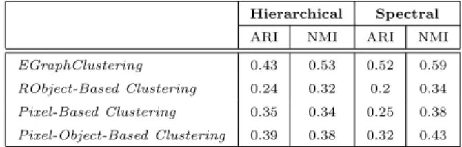
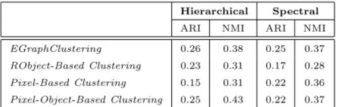
Table 1 and Table 2 provide the NMI and ARI values of the different ap-proaches over the Libron valley and the Lower Aude valley datasets respectively. We observe that the solution obtained using the reference objects (RObject-Based Clustering) always obtains the lowest performance. This result under-lines that considering how entities evolve over the time helps to discriminate among the different classes.
Considering the comparison between EGraphClustering, Pixel-Based Clus-teringand Pixel-Object-Based Clustering, we note that EGraphClustering clearly
ACCEPTED MANUSCRIPT
outperforms the different competitors, with both Hierarchical and Spectral clus-tering, on the Libron valley dataset (Table 1). Concerning the Lower Aude valley dataset (Table 2), we note that EGraphClustering obtains the best performances when the Spectral clustering method is used and even, when the Hierarchical clustering is used, it is still as efficient as all the other methods considering both NMI and ARI.
SITS datasets are different from standard time series data. Generally, time series analysis considers the temporal dimension to be the predominant feature while, in remote sensing analysis, spatial autocorrelation plays a role which is just as important as the temporal factor. Considering also the spatial evolution in order to differentiate among the different classes is crucial since the phenom-ena to be dealt with are fully spatio-temporal.
We would also stress that standard approaches to cluster time series of satel-lite images (Pixel-Based Clustering and Pixel-Object-Based Clustering ) only work at the pixel level while our framework directly manages object-based repre-sentations. Once the initial segmentation is performed, pixels are only employed to build the structure of the evolution graphs and any further operations are performed at the object level.
Hierarchical Spectral ARI NMI ARI NMI EGraphClustering 0.43 0.53 0.52 0.59 RObject-Based Clustering 0.24 0.32 0.2 0.34 Pixel-Based Clustering 0.35 0.34 0.25 0.38 Pixel-Object-Based Clustering 0.39 0.38 0.32 0.43
Table 1: Normalized Mutual Information and Adjusted Rand Index results of the different approaches for the Libron valley dataset employing two different clustering algorithms.
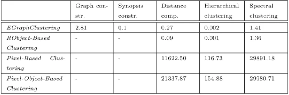
Table 3 and Table 4 summarize the time performances for the different ap-proaches over the Libron valley and the Lower Aude valley datasets respec-tively. For each method, we decompose the total running time. Considering the competing methods, the two major operations consist in pairwise distance matrix computation (Dist. comp.) and the execution of the clustering
algo-ACCEPTED MANUSCRIPT
Hierarchical Spectral ARI NMI ARI NMI EGraphClustering 0.26 0.38 0.25 0.37 RObject-Based Clustering 0.23 0.31 0.17 0.28 Pixel-Based Clustering 0.15 0.31 0.22 0.36 Pixel-Object-Based Clustering 0.25 0.43 0.22 0.37Table 2: Normalized Mutual Information and Adjusted Rand Index results of the different approaches for the Lower Aude valley dataset employing two different clustering algorithms.
rithm (Clustering ). Considering the EGraphClustering framework, two more steps need to be considered: the extraction of the evolution graphs (Graph. const.) and the construction of the synopsis representation for each of the graph (Synopsis constr.). We observe that when working with the same data, EGraphClusteringclearly requires less computational time than all pixel-based competitors. The RObject-Based Clustering approach requires less than a sec-ond to perform hierarchical clustering and about one secsec-ond for the spectral method. The EGraphClustering framework requires around one to two seconds to generate the final clustering solution for both algorithms while, all the pixel-based approaches require around 6 seconds for hierarchical clustering and more than 1 000 seconds for the spectral method on the Libron valley site. Consider-ing the Lower Aude valley site, the pixel-based strategies require more than 100 and 29 000 seconds for the hierarchical and the spectral clustering respectively. The hugely time-consuming computation behavior of pixel-based approaches is related to the use of pixels as basic unit for analysis. These result clearly high-light that our proposal seems more appropriate to the management and mining of huge time series of satellite images as it has proven to be more scalable, in terms of time behavior.
5.4. Qualitative results by Clusters Inspection
In order to better characterize the groups extracted by our approach, we did a manual inspection of the obtained clusters on the two study areas. The results are reported in Figures 5 to 8.
ACCEPTED MANUSCRIPT
Graph con-str. Synopsis constr. Distance comp. Hierachical clustering Spectral clustering EGraphClustering 0.36 0.02 0.05 0.003 1.04 RObject-Based Clustering - - 0.02 0.0007 0.96 Pixel-Based Clus-tering - - 1738.02 6.48 1185.30 Pixel-Object-Based Clustering - - 3013.02 6.04 1153.35Table 3: Time performance (in seconds) of the different approaches for the Libron valley dataset. Graph con-str. Synopsis constr. Distance comp. Hierarchical clustering Spectral clustering EGraphClustering 2.81 0.1 0.27 0.002 1.41 RObject-Based Clustering - - 0.09 0.001 1.36 Pixel-Based Clus-tering - - 11622.50 116.73 29891.18 Pixel-Object-Based Clustering - - 21337.87 154.88 29980.71
Table 4: Time performance (in seconds) of the different approaches for the Lower Aude valley dataset.
Libron valley. The evolution graphs in Figure 5(a) and Figure 5(b) belong to the same cluster while graphs in Figure 6(a) and Figure 6(b) belong to another cluster. The two clusters correspond to the Vineyards and Sclerophyll forest classes respectively. The color of a segment is related to the radiometric values associated to that object.
Considering the graphs related to the Vineyard cluster (Fig. 5(a) and Fig. 5(b)), we observe that, from a radiometric point of view, they have a similar behavior: at the beginning (T1and T2) and at the end (T5and T6) the spectral response
of these areas remain stable while, we observe a significant change in the middle of the time series (T3and T4). This temporal pattern is typical of agricultural
areas where a significant change occurs during the flowering season. Conversely, when we inspect the graphs belonging to the sclerophyll forest cluster (Fig. 6(a)
ACCEPTED MANUSCRIPT
and Fig. 6(b)), we note that a completely different behavior is shown. In this case, the spectral response of the Sclerophyll Forest areas remain stable. This can be explained by the behavior of this kind of vegetation. Sclerophyll forests grow slowly and a time series covering only a period of eight months cannot really depict the dynamics related to this kind of phenomena.
Figure 5: Evolution graph examples: two graphs of the vineyards cluster (a), (b) of Libron valleysite. The graph (a) represents the evolution of a vineyard plot identified at T5and the graph (b) represents the evolution of a vineyards plot identified at T3.
Figure 6: Evolution graph examples: two graphs belonging to the sclerophyll forest cluster (a), (b) of Libron valley site. The graph (a) represents the evolution of a sclerophyll forest area identified at T5and the graph (b) represents the evolution of a sclerophyll forest area identified at T2.
Figure 7: Evolution graphexamples: two graphs of the beach cluster (a), (b) of Lower Aude valley site. The graph (a) represents the evolution of a beach area identified at T4and the graph (b) represents the evolution of a beach area identified at T6.
Figure 8: Evolution graph examples: two graphes belonging to the lagoon cluster (a), (b) of Lower Aude valley site. The graph (a) and (b) represent the evolution of lagoon areas identified at T1.
Figure 7 and Figure 8 show four examples of evolution graphs from the Lower Aude valley. The graphs in Figure 7(a) and Figure 7(b) belong to the
ACCEPTED MANUSCRIPT
same cluster while graphs depicted in Figures 8(a) and 8(b) are, together, in a different cluster. In the case of the Lower Aude valley area, the two clusters correspond to the beach and lagoon classes respectively. Similarly, as highlighted in the previous scenario, the color of a segment is related to the radiometric values associated with it.
By analyzing the two representative graphs of the beach cluster (Fig. 7(a) and Fig. 7(b)), we note that the spectral response of this kind of area remains stable over time. This fact can be easily explained since the sand composing the beaches does not evolve over the eight months considered. The stable spatio-temporal behavior also impacts the structure of the graphs since the obtained evolution graphs, in this case, have a simple topology (a linear structure that is very close to a path). On the other hand, the two graphs representing the lagoon cluster (Fig. 8(a) and Fig. 8(b)) describe two spatio-temporal phenomena that clearly evolve over time. In both cases, we can observe that the radiometric responses change over time. Specifically, they remain stable in the beginning of the time series (T1, T2and T3) and then they change in the remaining time
stamps (T4, T5 and T6). The two evolution graphs represent a lagoon area
that is drying over time, at the end of winter the lagoon contains water while in the spring/summer period, due to different weather conditions, the water disappears and dry zones appear. When considering the topological structure of the two graphs, we can observe that, in the last part of the time series (August/September), both evolution graphs show complex structures since the original homogeneous spatial area is partitioned into different segments due to the emerging dry zones.
We performed similar analysis on other clusters. The findings we obtain are coherent with the examples discussed above. By manual inspection of the clustering results, we also observed that entities belonging to different classes share quite similar graph structures. The graph structure represents only the spatial evolution in terms of fragmentation between the segments of two succes-sive timestamps. This fact highlights that the graph-based representation alone, without the associated radiometric information, will probably not be enough to
ACCEPTED MANUSCRIPT
discriminate between different classes. 5.5. Method Applications
Our strategy is able to supply a compact and meaningful characterization of the underlying phenomena. The clustering result can be further analyzed by experts to detect common behaviors shared by different spatio-temporal entities that lie in the study area. The experimental results highlight that our frame-work can be employed by geographers as cold-start tool to remotely explore and summarize study areas where no previous knowledge is available. It can also support remote sensing researchers to prepare field campaign, thus saving human effort and reducing costs associated with field campaigns as it can be exploited to identify the most interesting areas to visit.
Furthermore, our framework can be used for environmental assessment and monitoring, to detect the affected area by deforestation, soil erosions and fires. The method offers a tool to understand how the areas are (seasonally) evolving and which zones are changing more. This kind of information combined with ecosystem models support the experts to identify the causes of these evolutions, forecast future changes and understanding the behavior of the area’s ecosystem. The framework can be used as well as for land use monitoring. In fact, in case of urban area, it can detect cities expansion and support land use planing tasks. Additionally it can be benefit for farmers to follow the crop growing, also to agricultural managers in order to prevent the socio-economic consequences of drought, climate changes or changes in the agricultural practices.
Finally, land use practices have a major impact on natural resources in-cluding water, soil, nutrients, plants and animals. Our framework can provide information to help developing solutions for natural resource management issues such as salinity and water quality.
6. Conclusion
In this paper, we have presented EGraphClustering, which is a novel frame-work for cluster spatio-temporal entities from SITS data by considering objects
ACCEPTED MANUSCRIPT
instead of pixels as basic unit of analysis. Our framework exploits a graph-based representation to describe spatio-temporal entities. It combines the evolution graph structure with the associated radiometric information to build a synopsis representation for each graph. The synopsis representation is successively ex-ploited to produce the pairwise distance matrix between each pair of evolution graphs. Finally, distance-based clustering algorithms can be leveraged to group together evolution graphs with similar behaviors. We assessed the performances of EGraphClustering on two real world remote sensing time series datasets and we have shown that our strategy outperforms standard pixel-based approaches regarding both clustering quality and computational time. As future work, we would like to investigate how we could adapt our framework to multi-year time series where recurrent phenomena can appear and how to distinguish recurrent spatio-temporal entities w.r.t. other kind of phenomena.
7. Acknowledgment
The authors wish to thank Algerian Ministry of Higher Education and Sci-entific Research and the French Space Study Center (CNES, Dynamitef 2016 TOSCA) for supporting this research. The authors acknowledge also the sup-port of the National Research Agency in the framework of the program ”In-vestissements d’Avenir” for the GEOSUD project (ANR-10-EQPX-20) for the distribution of the Landsat satellite images.
8. Bibliography
[1] S. Nativi, P. Mazzetti, M. Santoro, F. Papeschi, M. Craglia, O. Ochiai, Big data chal-lenges in building the global earth observation system of systems, Environmental Mod-elling and Software 68 (2015) 1–26.
[2] A. Julea, N. M´eger, C. Rigotti, E. Trouv´e, R. Jolivet, P. Bolon, Efficient spatio-temporal mining of satellite image time series for agricultural monitoring, Trans. MLDM 5 (1) (2012) 23–44.
ACCEPTED MANUSCRIPT
[3] W. Dorigo, R. de Jeu, Satellite soil moisture for advancing our understanding of earth system processes and climate change, Int. J. Applied Earth Observation and Geoinfor-mation 48 (2016) 1–4.
[4] G. E. A. P. A. Batista, E. J. Keogh, O. M. Tataw, V. M. A. de Souza, CID: an efficient complexity-invariant distance for time series, Data Min. Knowl. Discov. 28 (3) (2014) 634–669.
[5] T. Blaschke, Object based image analysis for remote sensing, ISPRS Journal of Pho-togrammetry and Remote Sensing 65 (1) (2010) 2–16.
[6] T. Lillesand, R. Kiefer, J. Chipman, Remote sensing and image interpretation (2008). [7] F. Guttler, S. Alleaume, C. Corbane, D. Ienco, J. Nin, P. Poncelet, M. Teisseire, Exploring
high repetitivity remote sensing time series for mapping and monitoring natural habitats - A new approach combining OBIA and k-partite graphs, in: IGARSS, 2014.
[8] Q. Zhu, G. E. A. P. A. Batista, T. Rakthanmanon, E. J. Keogh, A novel approximation to dynamic time warping allows anytime clustering of massive time series datasets, in: SDM, 2012, pp. 999–1010.
[9] T. Rakthanmanon, E. J. Keogh, S. Lonardi, S. Evans, Mdl-based time series clustering, Knowl. Inf. Syst. 33 (2) (2012) 371–399.
[10] F. Petitjean, J. Inglada, P. Gan¸carski, Satellite image time series analysis under time warping, IEEE Trans. Geos. and Rem. Sensing 50 (8) (2012) 3081–3095.
[11] F. Petitjean, C. Kurtz, N. Passat, P. Gan¸carski, Spatio-temporal reasoning for the clas-sification of satellite image time series, Pattern Recognition Letters 33 (13) (2012) 1805– 1815.
[12] T. Rakthanmanon, B. J. L. Campana, A. Mueen, G. E. A. P. A. Batista, M. B. Westover, Q. Zhu, J. Zakaria, E. J. Keogh, Addressing big data time series: Mining trillions of time series subsequences under dynamic time warping, TKDD 7 (3) (2013) 10.
[13] Z. Jiang, S. Shekhar, X. Zhou, J. Knight, J. Corcoran, Focal-test-based spatial deci-sion tree learning: A summary of results, in: Data Mining (ICDM), 2013 IEEE 13th International Conference on, IEEE, 2013, pp. 320–329.
[14] Z. Jiang, S. Shekhar, X. Zhou, J. Knight, J. Corcoran, Focal-test-based spatial decision tree learning, IEEE Transactions on Knowledge and Data Engineering 27 (6) (2015) 1547–1559.
[15] X. Li, C. Claramunt, A spatial entropy-based decision tree for classification of geograph-ical information, Transactions in GIS 10 (3) (2006) 451–467.
ACCEPTED MANUSCRIPT
[16] Z. Jiang, S. Shekhar, P. Mohan, J. Knight, J. Corcoran, Learning spatial decision tree for geographical classification: a summary of results, in: Proceedings of the 20th Inter-national Conference on Advances in Geographic Information Systems, ACM, 2012, pp. 390–393.
[17] V. V. Vazirani, Approximation Algorithms, Springer-Verlag New York, Inc., New York, NY, USA, 2001.
[18] P.-N. Tan, M. Steinbach, V. Kumar, Introduction to Data Mining, (First Edition), Addison-Wesley Longman Publishing Co., Inc., Boston, MA, USA, 2005.
[19] D. Ienco, R. G. Pensa, R. Meo, From context to distance: Learning dissimilarity for categorical data clustering, TKDD 6 (1) (2012) 1.
[20] J. R. Jr, R. Haas, J. Schell, D. Deering, Monitoring vegetation systems in the great plains with erts, NASA special publication 351 (1974) 309.
[21] B. Gao, Ndwi-a normalized difference water index for remote sensing of vegetation liquid water from space, Remote Sensing of Environment 58 (1996) 257–266.
[22] N. Zhang, Y. Hong, Q. Qin, L. Liu, N. Zhang, Y. Hong, Q. Qin, L. Liu, Vsdi: a visible and shortwave infrared drought index for monitoring soil and vegetation moisture based on optical remote sensing, International Journal of Remote Sensing 34 (2013) 4585–4609. [23] M. Baatz, Multiresolution segmentation: an optimization approach for high quality multi-scale image segmentation, Angewandte Geographische Informations verarbeitung XII (2000) 12–23.
[24] F. Pedregosa, G. Varoquaux, A. Gramfort, V. Michel, B. Thirion, O. Grisel, M. Blon-del, P. Prettenhofer, R. Weiss, V. Dubourg, J. Vanderplas, A. Passos, D. Cournapeau, M. Brucher, M. Perrot, E. Duchesnay, Scikit-learn: Machine learning in Python, Journal of Machine Learning Research 12 (2011) 2825–2830.