Time series representation for classification : a motif-based approach

(1)

HAL Id: tel-01922186

https://tel.archives-ouvertes.fr/tel-01922186

Submitted on 14 Nov 2018

HAL is a multi-disciplinary open access

archive for the deposit and dissemination of sci-entific research documents, whether they are pub-lished or not. The documents may come from teaching and research institutions in France or abroad, or from public or private research centers.

L’archive ouverte pluridisciplinaire HAL, est destinée au dépôt et à la diffusion de documents scientifiques de niveau recherche, publiés ou non, émanant des établissements d’enseignement et de recherche français ou étrangers, des laboratoires publics ou privés.

Xavier Renard

To cite this version:

Xavier Renard. Time series representation for classification : a motif-based approach. Data Struc-tures and Algorithms [cs.DS]. Université Pierre et Marie Curie - Paris VI, 2017. English. �NNT : 2017PA066593�. �tel-01922186�

(2)

THÈSE DE DOCTORAT DE

l’UNIVERSITÉ PIERRE ET MARIE CURIE Spécialité

Informatique

École doctorale Informatique, Télécommunications et Électronique (Paris) Présentée par

Xavier RENARD

Pour obtenir le grade de

DOCTEUR de l’UNIVERSITÉ PIERRE ET MARIE CURIE

Sujet de la thèse :

Time Series Representation for Classification:

A Motif-Based Approach

soutenue le 15 septembre 2017 devant le jury composé de :

Mme. Ahlame Douzal Rapportrice M. Louis Wehenkel Rapporteur M. Patrick Gallinari Examinateur M. Pierre-François Marteau Examinateur M. Themis Palpanas Examinateur M. Marcin Detyniecki Directeur de thèse Mme. Maria Rifqi Directrice de thèse M. Gabriel Fricout Encadrant industriel

(3)

(4)

Time Series Representation for Classification

A Motif-Based Approach

(5)

(6)

Abstract

Our research described in this thesis is about the learning of a motif-based representation from time series to perform automatic classification. Meaningful information in time series can be encoded across time through trends, shapes or subsequences usually with distortions. Approaches have been developed to overcome these issues often paying the price of high computational complexity. Among these techniques, it is worth pointing out distance measures and time series representations.

We focus on the representation of the information contained in the time series. We propose a framework to generate a new time series representation to perform classical feature-based classification based on the discovery of discriminant sets of time series subse-quences (motifs). This framework proposes to transform a set of time series into a feature space, using subsequences enumerated from the time series, distance measures and aggre-gation functions. One particular instance of this framework is the well-known shapelet approach.

The potential drawback of such an approach is the large number of subsequences to enumerate, inducing a very large feature space and a very high computational complexity. We show that most subsequences in a time series dataset are redundant. Therefore, a random sampling can be used to generate a very small fraction of the exhaustive set of subsequences, preserving the necessary information for classification and thus generating a much smaller feature space compatible with common machine learning algorithms with tractable computations. We also demonstrate that the number of subsequences to draw is not linked to the number of instances in the training set, which guarantees the scalability of the approach.

The combination of the latter in the context of our framework enables us to take advantage of advanced techniques (such as multivariate feature selection techniques) to discover richer motif-based time series representations for classification, for example by taking into account the relationships between the subsequences.

These theoretical results have been extensively tested on more than one hundred clas-sical benchmarks of the literature with univariate and multivariate time series. Moreover, since this research has been conducted in the context of an industrial research agreement

(7)

(CIFRE) with Arcelormittal, our work has been applied to the detection of defective steel products based on production line’s sensor measurements.

(8)

Résumé

Nos travaux décrits dans cette thèse portent sur l’apprentissage d’une représentation pour la classification automatique basée sur la découverte de motifs à partir de séries temporelles. L’information pertinente contenue dans une série temporelle peut être encodée temporelle-ment sous forme de tendances, de formes ou de sous-séquences contenant habituelletemporelle-ment des distorsions. Des approches ont été développées pour résoudre ces problèmes souvent au prix d’une importante complexité calculatoire. Parmi ces techniques nous pouvons citer les mesures de distance et les représentations de l’information contenue dans les séries temporelles.

Nous nous concentrons sur la représentation de l’information contenue dans les séries temporelles. Nous proposons un cadre (framework) pour générer une nouvelle représenta-tion de séries temporelles basée sur la découverte automatique d’ensembles discriminants de sous-séquences. Cette représentation est adaptée à l’utilisation d’algorithmes de classi-fication classiques basés sur des attributs. Le framework proposé transforme un ensemble de séries temporelles en un espace d’attributs (feature space) à partir de sous-séquences énumérées des séries temporelles, de mesures de distance et de fonctions d’agrégation. Un cas particulier de ce framework est la méthode notoire des « shapelets ».

L’inconvénient potentiel d’une telle approache est le nombre très important de sous-séquences à énumérer en ce qu’il induit un très grand feature space, accompagné d’une très grande complexité calculatoire. Nous montrons que la plupart des sous-séquences présentes dans un jeu de données composé de séries temporelles sont redondantes. De ce fait, un sous-échantillonnage aléatoire peut être utilisé pour générer un petit sous-ensemble de sous-séquences parmi l’ensemble exhaustif, en préservant l’information nécessaire pour la classification et tout en produisant un feature space de taille compatible avec l’utilisation d’algorithmes d’apprentissage automatique de l’état de l’art avec des temps de calculs raisonnable. On démontre également que le nombre de sous-séquences à tirer n’est pas lié avec le nombre de séries temporelles présent dans l’ensemble d’apprentissage, ce qui garantit le passage à l’échelle de notre approche.

La combinaison de cette découverte dans le contexte de notre framework nous permet de profiter de techniques avancées (telles que des méthodes de sélection d’attributs

(9)

variées) pour découvrir une représentation de séries temporelles plus riche, en prenant par exemple en considération les relations entre sous-séquences.

Ces résultats théoriques ont été largement testés expérimentalement sur une centaine de jeux de données classiques de la littérature, composés de séries temporelles univariées et multivariées. De plus, nos recherches s’inscrivant dans le cadre d’une convention de recherche industrielle (CIFRE) avec Arcelormittal, nos travaux ont été appliqués à la dé-tection de produits d’acier défectueux à partir des mesures effectuées par les capteurs sur des lignes de production.

(10)

Introduction

Time series data is everywhere: any measurement of a phenomenon over time produces time series. Every scientific discipline has many examples: physics and natural sciences provide large amounts of time series datasets with measurements of many parameters such as temperature, pressure, flow or concentration in meteorology, climatology, hydrology or earth science. In medicine, electrocardiogram (ECG) and electroencephalogram (EEG) are classical time series use-cases together with many other physiological parameters. In economics and in financial markets, stock market prices are notorious examples. In the industry, process monitoring produces massive amounts of sensor measurements. Time series represent our environment with large quantities of data that require the development of automatic techniques to analyze and extract the relevant information they contain.

Time series mining is the discipline dedicated to the development of such techniques, for the automatic discovery of meaningful knowledge from time series data. It provides techniques and algorithms to perform machine learning tasks on time series (classification, clustering, motif discovery, etc.). Time series mining exists as a specific field because time series have their own properties and challenges. In particular the meaningful information in the time series is encoded across time with trends, shapes or subsequences usually with distortions. Approaches have been developed to overcome these issues while the high computational complexity is handled: for instance, the core of most time series mining algorithms is composed of specific distance measures and time series representations.

This manuscript put an emphasis on the representation of the information contained in the time series. We have identified three main groups of time series representations: time-based representations (a raw time series is transformed into another time series that can be denoised, compressed and with the meaningful information highlighted), feature-based representations (a raw time series is transformed into a classical feature vector with features mainly derived from the feature analysis field, to characterize the structure of the time series for instance) and motif-based representations (meaningful subsequences

(15)

Figure 1.1: An example of time series: the observed globally averaged combined land and ocean surface temperature anomaly (from the 2014 Synthesis Report on climate change -Intergovernmental Panel on Climate Change)

(16)

13 are discovered from the time series: such subsequences can be recurrent, surprising or discriminant).

In this work, our objective is to develop a framework to learn subsequence-based rep-resentations from time series datasets to perform classification. One major drawback of existing classification strategies based on time series subsequences is their very high com-putational complexity. This complexity contributes to limit the expressiveness and the richness of the learned representation from the time series. This work aims to overcome the computational complexity issue to enable in practice the discovery of a rich subsequence-based time series representation for classification.

The theoretical developments of this work are benchmarked on industrial applications in the frame of a CIFRE agreement (industrial research agreement) with Arcelormittal, the worldwide market leader for steel production. Our proposition has been applied to the detection of defective products based on production line’s sensor measurements.

This manuscript is divided into three parts. The first part presents an overview of the time series mining field, the issues to perform machine learning on time series data and usual solutions developed in the literature. The second part details our proposition to learn a subsequence-based representation from time series meaningful for time series classification. The third part is about the evaluation of our approach on the industrial applications.

First part: state of the art to learn from time series

The first part of this manuscript is an overview of the time series mining field, with its challenges and solutions.

In Chapter 2 we detail the notation and the concepts used in the manuscript and we present the main time series mining tasks. Then, we expose the issues to train common machine learning algorithms on time series data and the common approaches to overcome them. Our work is focused on time series classification. We gather the time series classifica-tion approaches in two groups: time-based classificaclassifica-tion (based on distance measures) and feature-based approaches (based on suitable time series representations). Our work focuses on the second approach and more precisely on time series representations for classification: in chapter 3, we present an overview of the time series representation literature.

Second part: our proposition to learn a subsequence-based representation for time series classification

In the second part of this manuscript we introduce our proposition to learn subsequence-based representation for time series classification.

(17)

problem in chapter 5 to formalize a framework for the discovery of subsequence-based representation from time series to perform classification, which produces a classical feature vector suitable for machine learning algorithms. However, the computational complexity of the discovery on time series datasets prevents us to instantiate the framework on real world use-cases. In chapter 6, we demonstrate the possibility to reduce drastically this complexity thanks to the observation that many subsequences are redundant in a time series dataset. Finally, in chapter 7, we cast the discovery of the representation into a classical feature selection problem. Our proposition is evaluated through extensive experiments on more than one hundred datasets from the classical time series mining benchmark.

Third part: industrial applications

Our work is framed in a CIFRE agreement (industrial research agreement) with Arcelor-mittal. The evaluation of our proposition is presented in the third part of this work.

The industrial context, the use-cases and the datasets are presented in chapter 8. In chapter 9, our proposition is benchmarked on the industrial datasets. This chapter also illustrates the potential of subsequence-based representations, and our proposition in particular, to extract interpretable and relevant insights from the time series for process experts to perform further analysis.

We complete this manuscript by a conclusion and a discussion on the perspectives opened by this work.

(18)

Part I

Learning from Time Series

(19)

(20)

17 This part aims to provide the background for our proposition. Chapter 2 begins with a short introduction to the definitions and notations of the main concepts used in the work. Then, an overview of the time series mining field is provided, with a description of the main tasks of the domain. The application of common machine learning algorithms on time series is not straightforward: it raises several issues and challenges that will be discussed. In particular, we will see that a time series hardly fit in the classical static attribute-value model typical in machine learning [Kadous and Sammut, 2005]. Two typical ways to overcome these issues consist in the use of either adequate distance measures or the extraction or meaningful representations of the time series. Since our proposition is about the development of a representation based on subsequences, chapter 3 proposes an overview of the time series representations .

(21)

(22)

Chapter 2

Machine Learning on Time Series

In this chapter, we introduce the time series mining field. We begin with the definitions of the main concepts and notations used in this manuscript. Then, we propose an overview of the main time series mining tasks. Training machine learning models on time series raise issues. We will discuss them and describe two main strategies developed in the literature to overcome them: all time series mining approaches make use of time series representations and distance or similarity measures. Our work, and thus this manuscript, is mainly focused on time series classification.

2.1 Definitions & Notations

We introduce here the concept of time series and the notations used in this manuscript. A time series is an ordered sequence of real variables, resulting from the observation of an underlying process from measurements usually made at uniformly spaced time instants according to a given sampling rate [Esling and Agon, 2012]. A time series can gather all the observations of a process, which can result in a very long sequence. A time series can also result of a stream and be semi-infinite.

Machine learning techniques typically consider feature vectors with independent or uncorrelated variables. This is not the case with time series where data are gathered sequentially in time with repeated observations of a system: successive measurements are considered correlated and the time-order is vital [Reinert, 2010]. The correlation across time of the measurements lead to specific issues and challenges in machine learning, in particular to represent the meaningful information, usually encoded in shapes or trends spanning over several points in time.

Formally, we have a dataset D composed of N time series Tn such that D = {T1, . . . , Tn, . . . , TN}

(23)

Figure 2.1: Example of medical time series: an electrocardiogram (ECG). The relevant information in an ECG is encoded through shapes, thus successive points are correlated (from Wikimedia)

A time series Tn has a length L =| Tn | with Lmin ≤ L ≤ Lmax ∈ N* where Lmin is the smallest time series of D and Lmax is the longest one. Then a time series Tn is noted:

Tn= [Tn(1), . . . , Tn(i), . . . , Tn(L)]

A time series is univariate if for each timestep i the time series value is a scalar, usually a real number such that:

Tn(i) = x such that x ∈ R, ∀i ∈ [1 . . . L]

A time series is multivariate if for each timestep i the time series value is a vector of scalars, usually real numbers. The vector is of dimension M such that:

Tn(i) = [Tn,1(i), . . . , Tn,m(i), . . . , Tn,M(i)] such that Tn,m(i) ∈ R, ∀i ∈ [1, . . . , L] The variable m of a multivariate time series Tnis noted:

Tn,m = [Tn,m(1), . . . , Tn,m(i), . . . , Tn,m(L)]

A multivariate time series is described by a matrix L×M while a univariate time series is described by a vector of length L.

(24)

2.2. OVERVIEW OF THE TIME SERIES MINING FIELD 21

2.2 Overview of the time series mining field

The time series mining field can be seen as an instance of the data mining field applied to time series. It involves machine learning techniques to discover automatically meaningful knowledge from sets of time series. Some time series mining tasks, such as classification, perform predictions based on a representation of the time series. We propose in this section an overview of the different time series mining tasks.

2.2.1 Motif discovery

To introduce the motif discovery task we must define the concept of subsequence. A subsequence s is a contiguous set of points extracted from a time series Tn,m starting at position i of length l such that:

sTn,m(i, l) = [Tn,m(i), . . . , Tn,m(i + l − 1)]

A motif is a subsequence with specific properties. Motif discovery is the process that returns a motif or a set of motifs from a time series or a set of time series. Several types of motifs exist.

Recurrent motif A recurrent motif is a subsequence that appears recurrently in a longer time series or in a set of time series without trivial matches (overlapping areas) [Lin et al., 2002]. Recurrent motifs can also be defined as high density in the space of subsequences [Minnen et al., 2007], their discovery then consist in locating such regions.

Infrequent or surprising motif & anomaly detection An infrequent or surprising mo-tif is a subsequence that has never been seen or whose frequency of occurrence is significantly lower than other subsequences. Several concepts exist around this def-inition, such as the time series discords [Keogh et al., 2005, Keogh et al., 2007] defined as “subsequences maximally different to all the rest of the subsequences (...) most unusual subsequences within a time series” or defined as the detection of previ-ously unknown patterns [Ratanamahatana et al., 2010]. This kind of motif is related with anomaly detection in time series, which aims to discover abnormal subsequences [Weiss, 2004, Leng, 2009, Fujimaki et al., 2009], defined as a motif whose frequency of occurrence differs substantially from expected, given previously seen data [Keogh et al., 2002].

(25)

Figure 2.2: Recurrent motif: 3 similar subsequences can be identified in the time series (illustration from [Lin et al., 2002])

Task-specific relevant motif Motif discovery can be driven with a specific task in mind. For instance, it may be expected from discovered motifs to support a classification task. In this case, a motif or a set of motifs is said to be discriminant of class labels. The time series shapelet [Ye and Keogh, 2009] is one instance of this definition, among others [Zhang et al., 2009].

Many publications discuss the concept of time series motifs with often a proposition of algorithm. Such algorithms usually intend to solve the computational complexity of the motif discovery, since the naive discovery based on exhaustive subsequence enumeration is prohibitive [Keogh et al., 2002, Weiss, 2004, Mueen, 2013]. The precise definition of recur-rent, surprising or relevant is not obvious, many articles propose a criterion or a heuristic to detect motif among subsequences according to their own definition: the definition depends on the task to solve [Ratanamahatana et al., 2010]. A deeper review on motif discovery is performed in section 3.4.

(26)

Figure 2.3: Abnormal, surprising motif (illustration from [Keogh et al., 2005])

Figure 2.4: Examples of characteristic motifs to label motion types from an accelerometer sensor (illustration from [Mueen et al., 2011])

(27)

The motif is a central concept in time series mining since it allows the capture of temporal shapes.

2.2.2 Time series retrieval

Given a query time series Tn, time series retrieval aims to find the most similar time series in a dataset D based on their information content [Agrawal et al., 1993a, Faloutsos et al., 1994]. The querying can be performed on complete time series or on time series subsequences. In the latter case, every subsequence of the series that matches the query is returned. These two querying approaches are named respectively whole series matching and subsequence matching [Faloutsos et al., 1994, Keogh et al., 2001, Ratanamahatana et al., 2010]. Subsequence matching can be seen as a whole time series matching problem, when time series are divided into subsequences of arbitrary length segments or by motif extraction.

One major issue is the computational complexity of the retrieval. Many approaches have been proposed [Agrawal et al., 1993a, An et al., 2003, Faloutsos et al., 1997], and more recent ones [Wang et al., 2013b, Camerra et al., 2014, Zoumpatianos et al., 2016], based on a combination of time series representation (to reduce the dimensionality of the time series and accelerate the querying process) approximate similarity measures (to quickly discard irrelevant candidates without false dismissal, cf. lower bounding principle) and efficient indexing.

Time series retrieval has caught most of the research attention in time series mining [Esling and Agon, 2012].

2.2.3 Clustering

Time series clustering aims to find groups of similar time series in a dataset. These groups are usually found by assembling similar time series in order to decrease the variance inside groups of similar time series and increase the variance between them. A survey on time series clustering can be found in [Liao, 2005]. The main issue of most clustering approaches is to determine the number of clusters. Since clusters are not predefined, a domain expert may often be required to interpret the obtained results [Ratanamahatana et al., 2010].

Clustering is divided into whole sequence clustering and subsequence clustering [Ratanama-hatana et al., 2010]. In whole sequence clustering, the whole time series are grouped into clusters. When the raw time series are considered, specific distance measures can be used to handle distortions and length differences with classical clustering algorithms. In subsequence clustering, subsequences are extracted from time series to perform the cluster-ing. Literature suggests that extracting subsequences must be handled with care to avoid meaningless results [Keogh and Lin, 2005]. In particular, subsequence clustering may not

(28)

Figure 2.5: An example of time series clustering (illustration from [Wang et al., 2005]) provide meaningful results if the clustering is performed on the entire set of subsequences. Relevant subsequences should be extracted from the time series prior to clustering, for instance with a motif discovery algorithm [Chiu et al., 2003].

Time series clustering can be a stage for several other time series mining tasks, such as summarization or motifs discovery algorithm [Keogh et al., 2007].

2.2.4 Temporal pattern mining - Rule discovery

Rule discovery aims to relate patterns in a time series to other patterns from the same time series or others [Das et al., 1998]. One approach is based on the discretization of time series into sequences of symbols. Then association rule mining algorithms are used to discover relationships between symbols (ie. patterns). Such algorithms have been developed to mine association rules between sets of items in large databases [Agrawal et al., 1993b]. [Das et al., 1998], for instance, has extended it to discretized time series. Instead of association rules, decision tree can be learned from motifs extracted from the time series [Ohsaki and Sato, 2002].

2.2.5 Anomaly detection

Anomaly detection is defined as the problem of detecting “patterns in data that do not conform to expected behavior” [Kandhari, 2009]. In a previous paragraph, we mentioned the discovery of motifs on a definition based on abnormal subsequences. Motif is not the only way to label a time series as anomalous, other descriptors can be used. For instance, [Basu and Meckesheimer, 2007] propose an approach based on the difference of a point to

(29)

Figure 2.6: Example of time series classification: a dataset is composed by time series with cylinder, bell and funnel shapes. The task is to learn the information that discriminate these time series to label new time series (illustration from [Geurts, 2001])

the median of the other points in its neighborhood.

2.2.6 Summarization

A time series is usually long with complex information, an automatic summary may be useful to get insights on the time series. Simple statistics (mean, standard deviation, etc.) are often insufficient or inaccurate to describe suitably a time series [Ratanamahatana et al., 2010]. A specific processing has to be used to summarize time series. For instance, anomaly detection and motif discovery can be used to get a summary of the time series content: anomalous, interesting or repeating motifs are reported. Summarization can also be seen as a special case of clustering, where time series are mapped to clusters, each cluster having a simple description or a prototype to provide a higher view on the series.

Related with the summarization task, visualization tools of time series have been de-veloped in the literature (Time Searcher, Calendar-based visualization, Spiral, VizTree) [Ratanamahatana et al., 2010].

2.2.7 Classification

Time series data also supervised approaches, such as classification. Time series classifi-cation aims to predict a label given a time series in input of a model. The main task consists in the discovery of discriminative features from the time series to distinguish the classes from each other. Time series classification is used to perform for instance pat-tern recognition, spam filtering, medical diagnosis (classifying ECG, EEG, physiological measurements), anomaly or intrusion detection, transaction sequence data in a bank or detecting malfunction in industry applications [Ratanamahatana et al., 2010, Xing et al., 2010].

(30)

2.3. RELATIONSHIPS BETWEEN FIELDS 27

Weak Classification One single class is associated with a time series. It is probably the most common classification scenario in the literature. An example is shown figure 2.6.

Strong Classification Several labels can be used to describe with more granularity a time series. An example is the record of a patient’s health over time: various condi-tions may alternate from wealthy periods to illness along one time series describing a physiological parameter [Xing et al., 2010]. In this case a sequence of labels is associated with a time series instead of one single global label.

In the proposition of this work (part II) and in the industrial application (part III) we consider a weak supervised learning problem where each time series Tn is associated with exactly one class label y(Tn) ∈ C where C = {c1. . . c|C|} is a finite set of class labels and Y = [y(T1) . . . y(TN)].

2.3 Relationships between time series mining, time series

analysis and signal processing

Other scientific communities are involved in the development of techniques to process and analyze time series, for instance time series analysis and signal processing.

Time series analysis aims to develop techniques to analyze and model the temporal structure of time series to describe an underlying phenomena and possibly to forecast future values. The correlation of successive points in a time series is assumed. When it is possible to model this dependency (autocorrelation, trend, seasonality, etc.), it is possible to fit a model and forecast the next values of a series. Signal processing is a very broad field with many objectives: for instance to improve signal quality, to compress it for storage or transmission or detect a particular pattern.

Time series mining is at the intersection of these fields and machine learning: as we will see chapter 3, the application of machine learning techniques on time series data benefits from feature extraction and transformation techniques designed in other communities.

2.4 Time series mining raises specific issues

The tasks presented in the previous chapter are typical of the machine learning field, how-ever time series have specificities that prevent us to apply common approaches developed in the general machine learning literature. The reasons for this are discussed below.

(31)

2.4.1 A time series is not a suitable feature vector for machine learning

In general, a raw time series cannot be considered as suitable to feed a machine learning algorithm for several reasons.

In statistical decision theory, a feature vector X is usually a vector of m real-valued random variables such as X ∈ Rm_{. In supervised learning, it exists an output variable} Y, whose domain depends on the application (for instance a finite set of values Y ∈ C in classification or Y ∈ R in regression) such as X and Y are linked by an unknown joint distribution P r(X, Y ) that is approximated with a function f such as f(X) → Y . The function f is chosen according to hypothesis made on the data distribution and f is fitted in order to optimize a loss function L(Y, f(X)) to penalize prediction errors. The feature vector X is expected to be low-dimensional in order to avoid the curse of dimensionality phenomenon that affects performances of f because instances are located in a sparse feature-space [Hastie et al., 2009]. [Hegger et al., 1998] discusses the impact of high dimensionality to build a meaningful feature space from time series to perform time series analysis: with time series, the density of vectors is small and decreases exponentially with the dimension. To counter this effect an exponentially increasing number of instances in the dataset is necessary. Additionally, the relative position of a random variable in the feature vector X is not taken into account to fit f.

Time series data is by nature high dimensional, thousands points by instance or more is common. A major characteristic of time series is the correlation between successive points in time, with two immediate consequences. First, the preservation of the order of the time series points (ie. the random variables of X) is essential. Secondly, the intrinsic dimensionality of the relevant information contained in a time series is typically much lower than the whole time series dimensionality [Ratanamahatana et al., 2010], since they are correlated, many points are redundant.

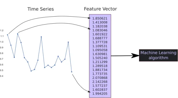
To illustrate the specific issues while learning from time series, let’s take a naive ap-proach. We consider the whole time series as a feature vector in input of any classical machine learning algorithm (decision tree, SVM, neural network, etc.). Each point of the time series is a dimension of the feature vector as illustrated figure 2.7.

A given dimension of X is expected to be a random variable with the same distribution across instances of the dataset. It means that time series have to be aligned across the dataset. This strong assumption is hard to meet for several reasons, in particular because of the distortions a time series can suffer.

• Time series from various dataset’s instances may not share the same length: the resulting feature vectors would not have the same number of dimensions.

It is usually not possible to change the input size of a machine learning algorithm on-the-fly. Each time series that doesn’t fit the input size would require an adjustment:

(32)

2.4. TIME SERIES MINING RAISES SPECIFIC ISSUES 29 Feature Vector 1.850621 1.413008 1.182038 1.083046 1.601922 1.688777 1.377728 1.109531 1.095058 1.630981 1.505240 1.211299 1.289518 1.881734 1.773735 2.070868 2.142268 1.577237 1.602837 1.994205 Time Series Machine Learning algorithm

Figure 2.7: A time series is set up as input vector of a machine learning algorithm without pre-processing

either truncating if too long or adding meaningless points (eg. zero padding) if too small. The consequences would be a loss of information in the first case and the addition of noise in the latter.

• Time series measure the occurrence of a phenomenon: the recording must have been performed with a perfect timing or a posterior segmentation of the time series is required to isolate the phenomenon from raw measurements to obtain a feature vector X where each dimension samples the same phenomenon’s stage across instances. For instance, if a set of time series store city temperatures, the first point of each time series must share the same time-stamp such as “January mean temperature” and so on. [Hu et al., 2013] highlights this issue: “literature usually assumes that defining the beginning and the ending points of an interesting pattern can be correctly identified while this is unjustified”. Also, the phenomenon of interest may be a localized subsequence in a larger time series. This subsequence may be out of phase across instances and appears at random positions in the time series. Figure 2.8 illustrates this point. The red motif, shifted, would appear in different positions in the feature vector. Motif discovery is a complex task and dedicated approaches are needed with processing steps to form a proper feature vector.

• A given phenomenon may occur at various speeds, frequencies and it may have slight distortions such as local accelerations, deceleration or gaps. While the shape of the motif would be similar, the points would be warped in time and would appear in

(33)

Figure 2.8: Two time series of various lengths recording a similar phenomenon described by the red motif

Figure 2.9: A similar motif of two time series but warped in time

different positions in the feature space (see Figure 2.9). A time series can suffer several types of distortions discussed section 2.5.1.

• A time series can be multivariate: the previous issues are reinforced in this case. Beside these issues and the curse of dimensionality, the high dimensionality of the time series is both a computing and a storage challenge. The information contained in a time series may be efficiently compressed using an adequate representation of the data. An adequate representation presents several advantages: beyond lower storage and computing requirements, a compact representation of the time series can ease the learning process by highlighting the relevant information and decreasing the dimensionality of the problem. The question of the representation of the time series information is discussed in detail

(34)

2.5. TRAIN MACHINE LEARNING ALGORITHMS ON TIME SERIES 31

chapter 3.

In the next section, we detail the main approaches developed in the literature to train machine learning algorithms from time series data to handle these issues.

2.5 Solutions to train machine learning algorithms on time

series

Training predictors from time series often requires a quantification of the similarity between time series. A predictor will try to learn a mapping to label or cluster identically similar time series. The issue is on what grounds to decide that time series content is similar. The literature offers many propositions, but as mentioned in [DeBarr and Lin, 2007] there is not one single approach that performs best for all datasets. The main reason resides in the complexity and the heterogeneity of the information contained in time series.

To compare time series, literature usually makes use of two complementary concepts: time series representation and distance measure.

• A time series representation transforms a time series into another time series or a feature vector. The objectives are to highlight the relevant information contained in the original time series, to remove noise, to handle distortions and usually to reduce the dimensionality of the data to decrease the complexity of further computations. A representation exposes the features on which time series will be compared. • A distance measure quantify the similarity between time series, either based on the

raw time series or their representations. In the latter case, all the time series must ob-viously share the same representation procedure. Complex distance measures usually aims to handle time series distortions.

Based on these two concepts, two main strategies emerge from the literature to apply machine learning algorithms on time series data. We call them time-based and feature-based approaches.

Time-based approaches consider the whole time series and apply distance measures on the time series to quantify their similarity. A time series representation can be used, it typically produces another time series of lower dimension to decrease the computational requirements.

Feature-based approaches transform the time series into a vector of features. The resulting time series representation is not yet a time series, but a set of features manually or automatically designed to extract local or global characteristics of the time series.

Figure 2.10 illustrates these concepts. The following sections present an overview of the two approaches. Since our work is focused on time series classification, we mainly review time-based and feature-based classification approaches.

(35)

Figure 2.10: based (also name instance-based) and Feature-based approaches. Time-based approaches compare the whole time series: suitable distance measures are crucial. Feature-based approaches extract representations of the information to generate features to feed typical machine learning algorithms (from [Fulcher and Jones, 2014])

2.5.1 Time-based classification

Time-based classifiers are suitable when the time series are well segmented on the phe-nomenon to describe so that a matching, performed over the whole time series in the time domain using distance measures, is relevant. This approach has a lot to do with time series retrieval. It has been claimed that one instance of the time-based classification, the nearest neighbor (k −NN), is difficult to beat when it is associated with the right distance measure to handle the time series distortions [Batista et al., 2011]. However, this approach assumes that the whole time series are comparable and thus perfectly segmented around the phenomenon of interest. A k − NN returns the k nearest time series in a dataset for an unobserved time series in input. Since the time series are associated with a label, the unobserved time series to label is associated with the majority class of its k neighbors. The 1 − NN in association with the Euclidean distance [Keogh and Kasetty, 2002] has been shown competitive in comparison with more complex distance measures (for eg. the Dynamic Time Warping -DTW) when the number of instances in the dataset is large [Ding et al., 2008].

Time-based classification requires from all the time series in the dataset to share the same length and the relevant patterns to be aligned. However, some distortions can be handled with suitable distance measures. In fact, most of the literature on time-based approaches focuses on distance measures to improve their capacity to handle misaligned time series and distortions using for instance elastic distance measures [Lines et al., 2014]. In the next paragraphs we propose a brief overview of the distortions a time series can suffer and the families of distance measures that have been developed to overcome them.

(36)

Time series distortions

Time series comes from real world measurements: similar time series will present distor-tions, in time or in amplitude, which will prevent us to identify them efficiently. In this section, we propose a brief overview of the distortions one can encounter with time series. The literature has many discussions on this topic, we rely on the overview by [Batista et al., 2011].

Difference of amplitude and offset Two time series can present similar shapes while their values are on different scales (see figure 2.11a). The phenomenon may not be measured in the exact same conditions (experimental conditions, measurement unit, etc.) or it may occurs with various amplitudes while the intrinsic shape is comparable. Some distance measures, such as the Euclidean distance, suffer from this kind of distortion and fails to identify similar time series with amplitude or offset differences. A normalization of each time series by their means and standard deviations (z-normalization) is suitable to address this distortion.

Time warping - Local scaling Two time series may present similar shapes but locally accelerated or decelerated (see figure 2.11c), this distortion is named time warping. One solution to address this distortion is the use of an elastic distance measure, for instance the Dynamic Time Warping (DTW).

Uniform scaling The uniform scaling can be seen as a simple case of the time warping where the whole time series is uniformly warped in time (the time series is stretched or com-pressed, see figure 2.11b). For instance, several time series measure a similar phenomenon that occurs at various (but constant) speeds or measured with a distinct sampling rate. The solution in this case is to find the factor to realign the time series [Keogh et al., 2004].

Phase invariance The phenomenon of interest may be randomly positioned in a time

series: the time series is not segmented precisely around this phenomenon because the starting bounds are not known. A more complex situation is the occurrence of several motifs randomly positioned in the time series (see figure 2.11d).

There are two solutions for this issue. Either the whole time series are comparable and all the possible alignments must be tested, or the time series would benefit from a representation in another space than the original time domain to extract the relevant information. For instance periodicities are well represented with a Fourier transform and subsequences can be extracted with motif discovery algorithms.

(37)

(a) Amplitude scaling (b) Uniform scaling

(c) Time warping - Local invariance (d) Phase invariance

(e) Occlusion invariance

(38)

Occlusion invariance [Batista et al., 2011] defines one last distortion, when part of the time series is missing (figure 2.11e). In this case, elastic distance measure is also suitable. Quantification of time series similarity

Given two time series, the issue is how to measure their similarity having in mind the noise and the distortions that can affect them. It is not straightforward to define a distance measure and decide which invariances to distortions should be enabled. An additional invariance property usually requires additional computation complexity and a distortion can be problematic for a use case but not for another one: the distance measure selection is linked with hypothesis on the information contained in the time series. For instance, a motif dilated in time may represents the same information in one case while it may not in another one. The distance measure may somewhat be considered as an hyper-parameter of the machine learning algorithm it serves.

For time-based comparison of time series, distance measures can be grouped into lock-step distances where the ith _{point of a time series is compared with the i}th _{of another time} series, and elastic distances that allow comparison of one point of a time series to several points of another one in order to handle distortions in time [Wang et al., 2013a].

Our objective in this section is not to be exhaustive on time series distance measures but rather to give some instances of the two families of distance measures: we advise the reader to refer to dedicated surveys such as [Ding et al., 2008, Wang et al., 2013a].

Lock-step distances The most commonly used distance measure for time-based

com-parison of time series is the Euclidean distance. It is easy to implement, compute and interpret [Keogh and Kasetty, 2002]. The Euclidean distance has also been shown com-petitive with more complex distances, especially for large datasets [Ding et al., 2008]. Formally, given two time series T1 and T2 of length L the Euclidean distance is given by:

d(T1, T2)L2 =

X_L

i=1 p

(T1(i) − T2(i))²

The drawback of the Euclidean distance is its sensibility to the distortions mentioned previously. Moreover it is unable to deal with time series of various lengths, even one point of difference since the comparison is made point by point. Amplitude distortions can be handled with transformation of the time series, such as the z-normalization ( handle difference of amplitude) or the Segmented Sum of Variations (SSV) [Lee et al., 2002]. Scale-invariant lock-step distances have also been proposed, such as the Minimal distance (Euclidean distance minus the time series’ offsets) [Lee et al., 2002] or the Mahalanobis distance [Arathi and Govardhan, 2014]. The correlation coefficient has also been used to take advantage of its scale invariance [Mueen et al., 2015].

(39)

Time-warping distortions are more complex to handle. Elastic distances, presented in the next section, have been proposed to tackle this issue.

Elastic distances

Dynamic Time Warping The major elastic distance is the Dynamic Time Warping

(DTW) [Berndt and Clifford, 1994]. Despite having been proposed decades ago, it has been shown competitive with more recent techniques [Wang et al., 2013a]. The DTW is able to compare time series with reasonable length differences and time distortions. The DTW principle consists in finding the best possible alignment between two time series, called a warping path, with the following rules:

1. The path must starts (ends) at the respective firsts (lasts) points of the two time series (boundary condition).

2. Every points of both time series must be used, and it is not possible to let aside one point of a time series (the continuity is required).

3. It is not possible to choose an alignment that would go backward in time (monotonic condition).

4. The warping path cannot be too steep or too shallow, to avoid the matching of two subsequences too different in length (slope constraint condition).

The main issue with DTW is its scalability. Its computation complexity in O(m2₎ (with m the time series length) makes the DTW up to 3 orders of magnitude slower than the Euclidean distance. The high computation complexity results from the search for a good time series alignment. Propositions have been designed to speed up the DTW. Many distance calculations can be pruned to avoid obvious non-solutions for the warping path. For instance, the first point of one time series can be immediately discarded as a possible association with the last point of the other time series. Global constraints on the warping path have been proposed to bound the possible warping paths. Two common strategies are the Sakoe-Chiba band and the Itakura Parallelogram. The constraints (or envelop around the warping path) can also be learnt, it has even been shown as improving the accuracy [Ratanamahatana and Keogh, 2004]. Other speedup techniques involves the DTW discovery on a low resolution representation of the time series, such as the PAA (see chapter 3) [Keogh and Pazzani, 2000].

DTW purpose is mainly to handle localized time warping. Some works propose the combination of DTW with other techniques to handle more time series distortions such as the uniform scaling [Fu et al., 2008a] or the use of an ensemble of elastic distance measures [Lines et al., 2014].

(40)

Figure 2.12: Comparison of flexible distance measures (including Dynamic Time Warping -DTW-) with the Euclidean distance (illustration from [Fu et al., 2008a])

(41)

Edit Distances The Edit Distances form another family of distance measures that are robust to temporal distortions. Edit distances have been developed in the bioinfor-matics and natural language processing fields to quantify similarity of two sequences of symbols. The idea is to evaluate the cost to transform one sequence to the other, by counting the minimum number of operations required [Moerchen, 2006]. The edition op-erations allowed are insertion, deletion and substitution of symbols, each operation has a specific cost associated. Since edit distances operate on symbolic sequences, the time series need to be transformed into a symbolic representation (see chapter 3). The most common edit distances for time series are the LCSS based on the Longest Common Subsequence principle, the Edit Distance on Real sequence (EDR) and the Edit Distance with Real Penalty.

2.5.2 Feature-based classification

The whole time series matching for classification may not be meaningful: it may be more relevant to match similar time series based on shared derived properties. In [Kadous and Sammut, 2005], authors highlight the difficulty to fit time series data into the classi-cal “static attribute-value model common in machine learning” as discussed section 2.4.1, which apart from designing a custom learner, let the practitioner with the option to ex-tract relevant features from the time series, at the price of a complex feature engineering stage. The temporal problem is transformed into a static problem with a static set of features [Fulcher and Jones, 2014]. For instance, similar time series may share the same global distribution of values well represented by its mean and standard deviation, or a global frequency content well represented by coefficients from a Fourier transform or more localized characteristics such as randomly localized subsequences well represented using a representation based on motif discovery. A large set of features can be extracted from time series to describe and represent the information they contain. In [Fulcher and Jones, 2014], authors extract thousands of features developed in the time series analysis field.

After a feature extraction step, the feature-based approach relies on classical machine learning algorithms that take a typical constant feature vector in input (Random Forest, SVM, Neural Networks...) to learn a mapping f from a constant representation of the time series and to perform the prediction.

While in the time-based approach the focus is set on a suitable distance measures, in the feature-based approach the issue is to find a representation that gathers a suitable set of features to represent the relevant information contained in the time series while handling the distortions.

(42)

2.6. CONCLUSIONS 39

2.6 Conclusions

In this chapter, we presented an overview of the time series mining field and we discussed the reasons why time series is a complex datatype that present issues to apply common machine learning techniques on them. Time series have specific properties and they are affected by distortions in amplitude and time.

We presented two main approaches to overcome these issues, appropriate distance mea-sures and time series representations. We also presented the typical ways to perform time series classification: we called the first approach time-based classification since the time series are compared as is using distance measures to overcome the distortions. We named the second approach feature-based classification: the principle is to discover and compute relevant representations of the time series information to train common classifiers.

In this work we focus on the discovery of meaningful time series representation to perform feature-based classification. The next chapter is dedicated to a review of the time series representations.

(43)

(44)

Chapter 3

Time Series Representations

As we have seen in the previous chapter, when it comes to learn from time series, we face four main issues. The first one is that time series is not a suitable “static attribute-value model” [Kadous and Sammut, 2005] that could enable to make a direct use of classical machine learning algorithms. The second issue is the distortions that affect time series. The third issue is the high dimensionality of the time series data that induces computational issues. The last issue is the heterogeneity of the information that can be stored in a time series. Learning a concept from a raw time series datasets is generally ineffective or even hopeless without a prior feature extraction step, designed with domain experts or with feature learning.

Two concepts allow us to handle these issues: the distance measures and the time series representations. Distance measures are mentioned in the previous chapter, here we focus on the representations. After a discussion on the time series representation principle, we propose an overview of the different types of time series representations with descriptions of some of their instances.

3.1 Concept of time series representation

The concept of time series representation is large and depends on the task to be solved and the approach used to do so. We define a time series representation Ψ as an operation that transforms a raw time series Tn into another time series ˆTn or a scalar xΨ (Tn) such that ˆTn or xΨ (Tn) summarizes a given feature in Tn.

Ψ (Tn) =          ˆ Tn or xΨ (Tn)

It may seems counter-intuitive to collect precise values of measurements to replace 41

(45)

them by an approximate representation. However, with time series we are generally not interested in the exact measure of each data point. The relevant information of a time series often relies on trends, shapes, motifs and patterns [Agrawal et al., 1993a] that may be better captured and described in an appropriate high-level representation that would additionally remove implicitly the noise [Ratanamahatana et al., 2010].

The objectives pursued by a time series representation is a combination of the following ones:

• Reduction of the dimensionality of the raw time series, to speedup the computations or reduce the computational needs. Many time series representations have been proposed in time series querying to obtain a transformed time series Ψ(Tn) of low dimensionality for a fast retrieval process.

• Reshape the time series to get it in a desired format, for instance a feature vector compatible with common machine learning algorithms. This feature vector should describe suitably the information contained in the time series.

• Summarization of the information contained in the time series.

• Accuracy of the representation to the raw time series, in particular for the retrieval task.

• Highlighting discriminative or characteristic information of the time series if the task is to perform classification, clustering or anomaly detection.

• Noise removal.

• Handling of time series distortions.

Many time series representations take origin or are related with techniques developed in the time series analysis and signal processing fields.

Several taxonomies exist to classify the time series representations, for instance the one proposed by [Esling and Agon, 2012], that groups time series representations into data adaptive and non-data adaptive representations.

We propose to sort the representations into 3 groups based on the type of information summarized and the format of the representation.

Time-based representations This group gathers representations that produce a time series from the whole raw time series, such as Ψ(Tn) = ˆTn. The time-based represen-tations are typically of lower dimensionality than T to speed up the compurepresen-tations. Feature-based representations This group gathers representations that produce a scalar

(46)

3.2. TIME-BASED REPRESENTATIONS 43

It is for instance the case of representations of time series by the description of the global distribution of the values, the global trends or the global frequency content. Motif-based representations This group gathers representations that produce a time

series from the whole raw time series, such as Ψ(Tn) = ˆTnbut unlike time-based rep-resentations, the resulting time series is a subsequence, extracted from the raw time series based on desired properties, for instance recurring, abnormal, discriminative subsequences or sequences of subsequences.

Feature-based representations and time-based representations are often time-series-focused: the representation is computed independently by time series. Motif-based representations are more often dataset focused: motifs are discovered at dataset scale.

In the following sections, we illustrate the concept of representation with instances from each group. The reader must remember that the literature on time series representations is very large and this review doesn’t intend to be exhaustive.

3.2 Time-based representations

Time-based representations represent time series by preserving the temporality or at least the sequentiality of the data, typically by computing an approximation of some feature at local scale. Many time-based representations exist, they are mainly used to perform fast time series retrieval, querying or indexing. They can also be used for whole time series classification (time-based classification, see section 2.5) to accelerate the classification and to be invariant to some distortions.

We can group the time-based representations according to the type of transformation applied to the data [Bettaiah and Ranganath, 2014].

• Piecewise representations: the time series is segmented then a local feature is com-puted for each segment (for eg. the mean, average rate of variations or a regression coefficient).

• Symbolic representations: the time series is segmented and then discretized. A dic-tionary of symbols is either learned or applied in order to convert the time series into a series of symbols.

• Transform-based representation: the time series is converted from the time domain into another domain (for eg. the time-frequency domain thanks to a wavelet trans-form).

(47)

3.2.1 Piecewise Representations

Piecewise Representations (PR) aim to represent time series by reducing their dimension-ality thanks to the segmentation of the time series followed by a representation of each segment by a value. The time series representations falling in this category can be sorted according to two axis:

• The segmentation process: there are adaptive and non-adaptive segmentation tech-niques.

• The representation of each segment: which feature or set of features is extracted to represent each segment. The number of possibilities for this axis is large. It is somehow shared with the feature-based representations, which operates at the global scale of the time series (see section 3.3).

We present here several illustrative Piecewise Representations, each of them with a specific pair of segmentation technique and segment’s summarization technique. Representations are grouped according to their segmentation technique (adaptive or not). We begin with the simpler time series dimensionality reduction technique, a basic sub-sampling, to illustrate the challenges.

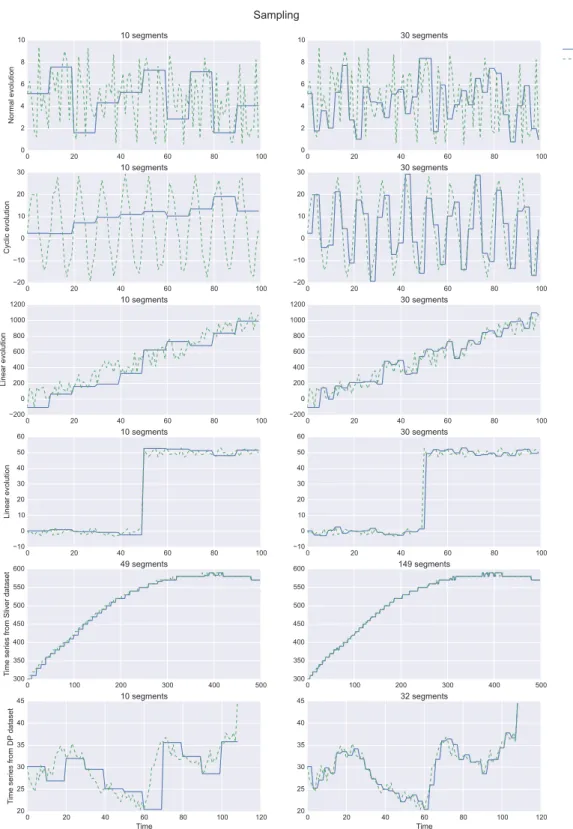
Sub-Sampling

The simpler PR is probably the basic sub-sampling of the time series. One value is con-served every h points of the time series. The sub-sampling method summarizes every segment of h points of the time series by the value of one single arbitrary point of the segment. The only constraint on h is to respect the Nyquist frequency theorem that states that no information is preserved over the Nyquist frequency after the sub-sampling. The N yquist frequency is given by [Åström, 1969]:

fc= 1 2h

Sub-sampling is mainly used in signal processing when a continuous signal has to be converted into a discrete one. A signal can also be re-sampled when its acquisition fre-quency is higher than the one required by the Nyquist frefre-quency theorem to represent the phenomenon by the time series.

A sub-sampled time series allows faster computations and less storage requirements. The method is easy to implement: the only parameter is h. However, the main drawback of sub-sampling is the distortion of the time series shape if the sampling rate is too low to depict the underlying phenomena [Fu, 2011]. When performing time series mining we usually ignore the information to be discovered, thus the Nyquist frequency is hard to guess to further determine the parameter h. Moreover, the discarded points are completely

(48)

3.2. TIME-BASED REPRESENTATIONS 45

ignored during the representation process, important patterns may be missed. To represent complex shapes, the required number of points with this approach may be high, with no or few improvements for computation and storage.

Non-adaptive segmentation

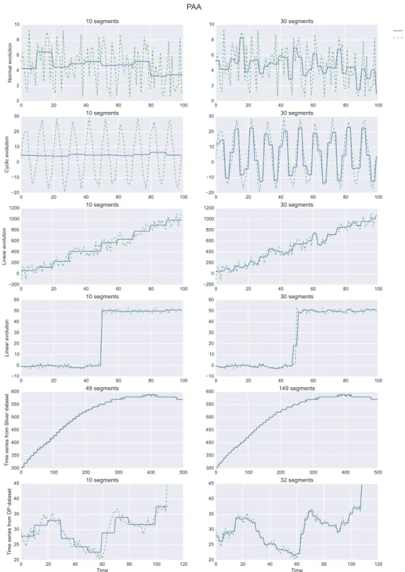
The Piecewise Aggregate Approximation (PAA) is maybe the most important time-based representation based on non-adaptive segmentation. It can be seen as an enhancement of the sub-sampling method. Instead of representing each segment of length h by its first value, the PAA summarizes the segment by its mean, expecting a higher fidelity in the representation of each segment [Keogh et al., 2001, Yi and Faloutsos, 2000].

A time series Tn of length L is segmented into N fixed-length segments. For each segment, the mean value is computed to represent the segment. Tn is then reduced to an approximate time series ˆTn= [ ˆTn(1), . . . , ˆTn(i), . . . , ˆTn(N )] of length N. PAA has one single parameter that is the length N of ˆTn.

Each point of ˆTn is computed as: ˆ Tn(i) = N L L Ni X j=_NL(i−1)+1 ˆ Tn(j)

The PAA has several drawbacks. The first one is the hypothesis made to represent the information. PAA assumes the information is suitably represented by the mean over one segment, which is not often the case. Variations of the PAA have been proposed to address this point such as [Quoc et al., 2008] that adds slope information to the mean for each segment, [Guo et al., 2010] adds variance to the mean. [Lee et al., 2002] proposes the Segment Sum of Variation representation (SSV ) that computes the variation between two adjacent points, each segment is represented by the sum of variations within the segment. One advantage of the SSV is its invariance to amplitude and offset distortion. If two time series present different means, their shape can be compared directly with the SSV representation without any prior preprocessing (such as scaling or normalization of the data) or without any particular distance measure (such as the minimum distance, the Euclidean distance between two time series minus the mean distance between the two series). Two time series represented with SSV and with a similar shape but a distinct offset can be compared directly with Euclidean distance [Lee et al., 2002].

Another drawback is the resolution of the information: the segment size is fixed and one value summarizes the whole segment whatever the resolution of the shapes and trends in the time series. Th Multi-Resolution PAA (MPAA) has been proposed to compute several PAA representations of the same time series at various resolutions. At the first level, a typical PAA is computed on the raw time series. The process is recursively applied on the

(49)

0 20 40 60 80 100 0 2 4 6 8 10 No rma l e vo lu ion 10 segmen s 0 20 40 60 80 100 0 2 4 6 8 10 30 segmen s Represen a ion Raw signal 0 20 40 60 80 100 −20 −10 0 10 20 30 Cycl ic evo lu ion 10 segmen s 0 20 40 60 80 100 −20 −10 0 10 20 30 30 segmen s 0 20 40 60 80 100 −200 0 200 400 600 800 1000 1200 Lin ea r e vo lu ion 10 segmen s 0 20 40 60 80 100 −200 0 200 400 600 800 1000 1200 30 segmen s 0 20 40 60 80 100 −10 0 10 20 30 40 50 60 Lin ea r e vo lu ion 10 segmen s 0 20 40 60 80 100 −10 0 10 20 30 40 50 60 30 segmen s 0 100 200 300 400 500 300 350 400 450 500 550 600 Time se rie s f rom Sli ve r d a a se 49 segmen s 0 100 200 300 400 500 300 350 400 450 500 550 600 149 segmen s 0 20 40 60 80 100 120 Time 20 25 30 35 40 45 Time se rie s f rom DP da ase 10 segmen s 0 20 40 60 80 100 120 Time 20 25 30 35 40 45 32 segmen s Sampling

Figure 3.1: Several time series shapes and their associated representations using sub-sampling representation